FULL PAPER
V
S30
, slope,
H
800
and
f
0
: performance
of various site-condition proxies in reducing
ground-motion aleatory variability
and predicting nonlinear site response
Boumédiène Derras
1,2*, Pierre‑Yves Bard
3and Fabrice Cotton
4,5Abstract
The aim of this paper is to investigate the ability of various site‑condition proxies (SCPs) to reduce ground‑motion aleatory variability and evaluate how SCPs capture nonlinearity site effects. The SCPs used here are time‑averaged shear‑wave velocity in the top 30 m (VS30), the topographical slope (slope), the fundamental resonance frequency (f0) and the depth beyond which Vs exceeds 800 m/s (H800). We considered first the performance of each SCP taken alone and then the combined performance of the 6 SCP pairs [VS30–f0], [VS30–H800], [f0–slope], [H800–slope], [VS30–slope] and [f0–H800]. This analysis is performed using a neural network approach including a random effect applied on a KiK‑net subset for derivation of ground‑motion prediction equations setting the relationship between various ground‑motion parameters such as peak ground acceleration, peak ground velocity and pseudo‑spectral acceleration PSA (T), and Mw, RJB, focal depth and SCPs. While the choice of SCP is found to have almost no impact on the median ground‑ motion prediction, it does impact the level of aleatory uncertainty. VS30 is found to perform the best of single proxies at short periods (T < 0.6 s), while f0 and H800 perform better at longer periods; considering SCP pairs leads to signifi‑ cant improvements, with particular emphasis on [VS30–H800] and [f0–slope] pairs. The results also indicate significant nonlinearity on the site terms for soft sites and that the most relevant loading parameter for characterising nonlinear site response is the “stiff” spectral ordinate at the considered period.
Keywords: Aleatory variability, Site‑condition proxies, KiK‑net, Neural networks, GMPE, Nonlinear site response
© The Author(s) 2017. This article is distributed under the terms of the Creative Commons Attribution 4.0 International License (http://creativecommons.org/licenses/by/4.0/), which permits unrestricted use, distribution, and reproduction in any medium, provided you give appropriate credit to the original author(s) and the source, provide a link to the Creative Commons license, and indicate if changes were made.
Introduction
Probabilistic seismic hazard analysis (PSHA) strongly relies on ground-motion prediction equations (GMPEs) that quantify the amplitude of ground motion as a func-tion of distance, magnitude and site-condifunc-tion prox-ies (SCPs). The latter are introduced to characterise the amplification effects linked to near-surface deposits. Given the variety of physical phenomena impacting the characteristics of an earthquake shaking, ground-motion models include a large degree of uncertainty. This uncer-tainty (especially the within-event aleatory variability)
is strongly affected by near-surface site conditions. An important question is the degree to which this scatter can be reduced by improvements in the way to account for the near-surface effects. The incorporation of those effects in GMPEs has gone through an evolution in the
past years (Chiou and Youngs 2008; Seyhan et al. 2014;
Derras et al. 2016). At the beginning, ground-motion
models typically contained a scaling parameter based
on site classification (e.g. Boore et al. 1993) or presented
different models for “hard rock” and “soil” sites (e.g.
Campbell 1993; Sadigh et al. 1997). Boore et al. (1997)
introduced the explicit use of the time-averaged
shear-wave velocity in the top 30 m (VS30). VS30 has become
de facto a standard for the development of GMPEs and seismic hazard assessment at national and international scales. In this way, it has been observed (e.g. Borcherdt
Open Access
*Correspondence: [email protected]‑tlemcen.dz
1994) that VS30 is a useful parameter to predict local site amplification in active tectonic regimes, especially when
it is actually measured: Derras et al. (2016) showed after
Chiou and Young (2008) that measuring VS30 allows a
sig-nificant reduction in the aleatory variability.
VS30 has certainly proved to constitute a simple and
effi-cient SCP metric, but it also proved not to be a low-cost SCP, as it is far from being measured at all strong-motion sites throughout the world (except in Japan). For this
rea-son, Wald and Allen (2007) and Allen and Wald (2009)
have proposed to use the topographical slope (slope) from digital elevation models (DEMs) derived from remote sensing (satellite imaging) to give a first-order
estimation of site classes based on VS30. Many other ways
to infer VS30 values without measuring them have been
proposed, as listed in Seyhan et al. (2014): extrapolation
from VS measurements at depths shallower than 30 m,
correlations—more or less robust—with other types of information or parameters (geology, geomorphological or terrain-related proxies, geotechnical parameters).
On the other hand, VS30 alone cannot satisfactorily
pre-dict the amplification for sites underlain by deep sedi-ments, which require knowledge of the geology to depths
greater than 30 m (e.g. Choi and Stewart 2005; Luzi et al.
2011). Campbell (1989) found that adding a parameter
for depth to basement rock improved the predictive abil-ity of empirical ground-motion models. On their side,
Cadet et al. (2011) and Derras et al. (2012) used another
SCP: the fundamental resonance frequency, f0, as
deter-mined by the horizontal-to-vertical (H/V) spectral ratio
technique (Mucciarelli 1998; Haghshenas et al. 2008;
Bard et al. 2010). As the f0 (H/V) SCP is able to identify
low-frequency amplification on thick sites, its relevance may be compared with the performance of another SCP often proposed to properly account for the sediment
thickness, H800 (depth beyond which the shear-wave
velocity exceeds 800 m/s).
The main aim of this work was to assess the actual
per-formance of several site-condition proxies, namely VS30,
slope, f0 (H/V) and H800 SCP, by analysing the relative
decrease in the ground-motion aleatory variability each of them allow to achieve and by investigating the benefits of considering simultaneously multiple site proxies. In addition, as all the considered ANN models were found to predict a significantly nonlinear site response, a sec-ondary aim has been to investigate to which extent these SCPs allow to capture not only the linear, but also the nonlinear nature of site response, in combination with various loading parameters (PGA on rock, acceleration response spectrum at the period of interest PSA (T), or a
site-related strain proxy PGV/VS30.
The KiK-net database used here consists of shallow crustal events recorded on sites for which several site
proxies are already available: VS30 and H800 values can be
directly derived from downhole measurements of VS
pro-file (Dawood et al. 2014), the slope values have been
com-piled (Ancheta et al. 2014), and f0 values are taken from
Régnier et al. (2013). The KiK-net data offer the unique
opportunity to have, for each strong-motion recording, a reliable measurement of the four SCPs, thus allowing a thorough and meaningful comparative assessment of the performance of each of these proxies.
The artificial neural network (ANN) approach and a
random-effect-like procedure (Derras et al. 2014) have
been used for the derivation of GMPEs setting the rela-tionship between various ground-motion parameters [peak ground acceleration (PGA), peak ground veloc-ity (PGV) and 5% damped pseudo-spectral acceleration (PSA) from 0.01 to 4 s] and event/station
meta-parame-ters (moment magnitude Mw, Joyner and Boore distance
RJB, focal depth and site-condition proxies VS30, slope,
H800 and f0).
After a short presentation of the data set, a section is dedicated to the presentation of the ANN models and their specific implementation for deriving GMPEs. The following section presents the results obtained for the KiK-net data, focusing on (a) the respective performance of each of the four site proxies which are considered either alone or within combinations and (b) a discussion of their ability to detect and account for nonlinear site response.
Data set
The Kiban–Kyoshin network (KiK-net) is one of the two national strong-motion seismograph networks devel-oped in Japan following the 1995 Kobe earthquake. The KiK-net is a network of strong-motion instruments that consist of about 700 stations with an average spacing of about 20 km distributed throughout the Japanese islands
(Hayashida and Tajima 2007). The KiK-net stations are
each equipped with a pair of surface and downhole, sen-sitive three-component digital accelerometers, allow-ing an empirical evaluation of the site response at each station.
The resulting data set considered here has been
com-piled by Dawood et al. (2014, 2016). This data set has
been downloaded from https://datacenterhub.org/
resources/272. The corresponding data processing is fully
described in Dawood et al. (2014, 2016). In short, this
data processing includes several steps: baseline
correc-tion, tapering on both ends (total length of tapering = 5%
of the total record length), zero padding before and after
recommended by Boore (2005) in relation to the order
and frequency of the high-pass filtering, fourth-order acausal Butterworth filtering with selection of the
displacement values at the end of the time series remain smaller than some magnitude-dependent thresholds,
sig-nal-to-noise ratio larger than 3 between 2 fc and 30 Hz.
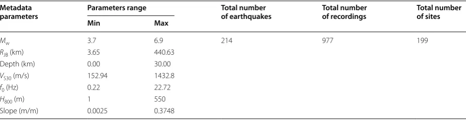
The data set using here contains 977 recordings from
199 sites to 214 earthquakes. The range of Mw, RJB, depth
and all SCPs is listed in Table 1, which also provides
the number of earthquakes, records and sites. The cor-responding range of recorded PGA values spans from
2.6 × 10⁻⁴ to 0.41 g.
Site‑condition proxies
The chosen site proxies are VS30 and slope, which are
generally considered a priori as more relevant for
short-period ground motions, and f0 (H/V) and H800, that
should in principle be more suitable for long periods. There actually exist several possibilities proposed by dif-ferent authors for such a sediment thickness parameter. It is true that most recent NGA-West and NGA-West 2 GMPEs use depths corresponding to larger velocities, as
indicated by the reviewer. We have chosen to select H800
as a thickness parameter for the following reasons:
• The database used in this study provides only the
H800 values. H2500 and H1100 values are not available
yet in this database.
• The ongoing revision of European building codes
recommends the use of both VS30 and H800 for site
classification, since the “rock” sites are
convention-ally associated with VS30 values exceeding 800 m/s.
Results associated with H800 are then of interest of
many colleagues.
The larger the target velocity, the larger the uncertainty on the corresponding depth: even in very well-known areas such as California, the different existing models
lead to highly variable H2500 values (see Figure 10 in
Sey-han et al. 2014). H800 thus seems an acceptable
compro-mise, especially as we do not look for “basin” effects (i.e. including 2D or 3D very-low-frequency effects, such as
those existing in the Los Angeles area or Kanto plain), but simply for a parameter that helps to constrain the intermediate response (around 1 s).
Ground-motion models are derived first using one
single SCP [one model with each of the four values: VS30
or slope or f0 or H800] and then using two SCPs out of
the four [i.e. six models in total with the six pairs (VS30,
slope), (VS30, H800), (VS30, f0), (H800, slope), (f0, H800) and
(slope, f0)]. All SCPs are considered through their log10
values. In addition, two reference ground-motion models are established for comparison with each of the 10 previ-ous ones: the first one is without any site proxy (named “without site proxy”), and the second one considers simultaneously all four site proxies (named “all proxies”) to estimate the maximum possible standard deviation reduction.
Data distribution
The distribution of the data set according to Mw, RJB,
focal depth, PGA and site-condition proxy (SCP) is
dis-played in Figs. 1 and 2.
Figure 1 shows the distributions of the KiK-net data set
in the magnitude–distance plane by bins of PGA and in
the PGA–distance plane by bins of Mw. The distributions
are given for all site conditions (left column), but also
for soft sites only (VS30 < 300 m/s, middle column) and
stiff sites only (VS30 > 800 m/s, right column). The goal
of these presentations by bins of Mw, PGA and VS30 is
to ensure that the data distribution is appropriate for all
Mw–PGA and for soft and stiff soils. This figure also
illus-trates clearly the much smaller number of recordings at distances less than 10 km in general and less than 30 km when only stiff-to-rock sites are considered.
Figure 2 represents the cumulative distribution
func-tion (CDF) of the used data set versus RJB, Mw, VS30,
topographical slope, H800, f0, focal depth and PGA. The
four SCP distributions are found to follow a lognormal
distribution as well as RJB and PGA, while Mw and focal
depth are much closer to a normal distribution (see also
Table 1 Range of magnitude, distance and site-condition proxy for the KiK-net subset considered in this study Metadata
parameters Parameters range Total number of earthquakes Total number of recordings Total number of sites
Min Max
Mw 3.7 6.9 214 977 199
RJB (km) 3.65 440.63
Depth (km) 0.00 30.00
VS30 (m/s) 152.94 1432.8
f0 (Hz) 0.22 22.72
H800 (m) 1 550
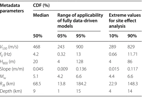
Figure 2 in Derras et al. 2016). In our ANN models, we thus used the logarithm (base 10) values of all SCPs and
spectral ordinates PSAs. Table 2 details a fractile values
for each of these metadata parameters: median value, 5 and 95% fractiles which are considered to provide the range of applicability of the models, and the 10 and 90% fractiles which will be used in the following to estimate the impact of each SCP on the site amplification factor.
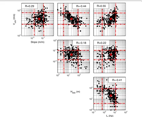
To ensure that the SCPs are not strongly dependent on one another, correlation plots are displayed for each
pair of SCPs (Fig. 3) together with the corresponding
cor-relation coefficient (R). Although some pairs do exhibit
some correlation (Rmax = 0.55 between VS30 and f0), the
scatter is large enough for the SCPs to be considered as almost independent site parameters for the derived ANN models. The weakest correlation is found between slope
and either H800 or f0. One may notice that H800 is
nega-tively correlated with the three other SCPs: the larger
it is, the lower are f0, VS30 and slope—as could be
intui-tively expected. In the same figure are also indicated the median values and the 10 and 90% fractiles for the all SCPs.
Methods
The random-effect regression algorithm made popu-lar within engineering seismology by Abrahamson
and Youngs (1992), which is arguably the most
com-monly used approach for developing empirical ground-motion models. In our ANN models, we used this type of approach in order to facilitate the comparability with classical GMPEs. The ANN has the advantage that no
prior functional form is needed (Derras et al. 2012): the
actual dependence is established directly from the data and can therefore be used as a guide for a better under-standing of the factors which control ground motions. This resulted in a two-phase building process.
Fixed models
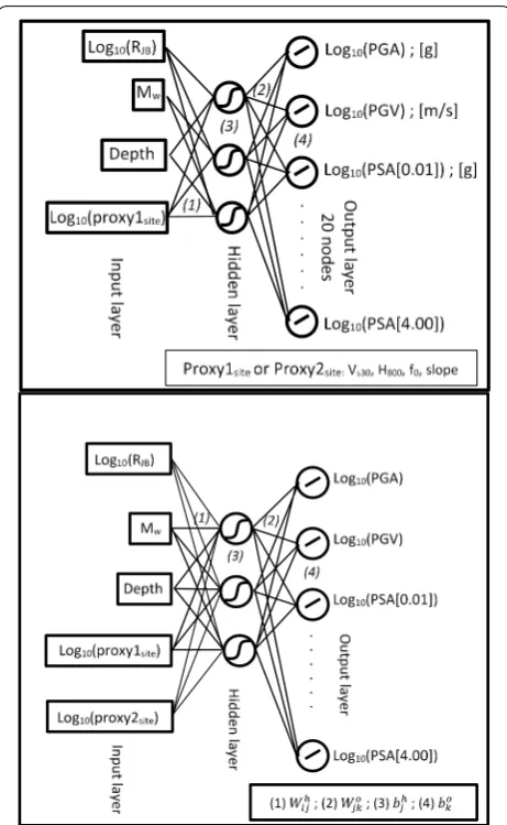
The architecture of ANN used in this work is named “feedforward network”, consisting of a series of layers. The first layer ensures the connection with the input
parameters, i.e. in our case Mw, RJB and depth and one
or two (or possibly more) continuous parameter
describ-ing the SCPs (VS30, slope, f0, H800). Each subsequent layer
has a connection from the previous layer. The final layer produces the network’s output. A feedforward network with one hidden layer and three neurons in the hidden layer is adopted in this study. This small number of hid-den neurons is the optimal number in order to optimise both the total standard deviation of residuals σ and the
Akaike information criterion (Akaike 1973). Figure 4
illustrates a typical architecture of the ANN-fixed models 4
Vs30<300 m/s Vs30>800 m/s
Vs30<300 m/s
All Vs30 Vs30>800 m/s
All Vs30
Fig. 1 Distribution of the KiK‑net data set considered in this study. The three top plots correspond to the magnitude (Mw)–distance (RJB) distribu‑ tion. For these three plots, the bins with different colours correspond to seven sample‑size subsets with increasing PGA values from 0.001 to 1 g. On the three bottom plots, the distribution of PGA versus distance (RJB) is shown. In these plots, the distribution is given by bins of Magnitude,
which were implemented within the MATLAB®
Neu-ral Network Toolbox™ (Demuth et al. 2009). The output
layer groups all the considered ground-motion param-eters, i.e. the classical geometric mean of the horizontal components of PGA, PGV and 5%-damped PSA at 18 periods from 0.01 to 4 s. We did not include predictions for peak ground displacement (PGD), which we consider to be too sensitive to the high-pass filters used in the data processing.
Quasi-Newton back-propagation technique also called “BFGS” (Broyden–Fletcher–Goldfarb–Shanno) has been
applied for the training phase (Shanno and Kettler 1970).
To avoid “overfitting” problems, we chose an adequate regularisation method involving the modification of the conventional mean sum of the squares of the network errors by the addition of a term equal to the sum of the
101 102
0 0.5
1 Empirical CDF
RJB (km)
4 5 6
Mw
1000 0
0.5 1
Vs30 (m/s)
10-2 10-1
Slope (m/m)
100 102
0 0.5 1
H800 (m)
1 10
f0 (Hz)
0 10 20
0 0.5 1
Depth (km)
10-3 10-2 10-1
PGA (g)
Fig. 2 Empirical cumulative distribution function (CDF) versus the explanatory variables RJB (top left), Mw (top right), VS30 (first middle left), slope (first middle right), H800 (second middle left), f0 (second middle right), depth (bottom left) and the response PGA variable (bottom right) for the considered KiK‑net data set
Table 2 Metadata range for site effect analysis and for fully data-driven models applicability
Metadata
parameters CDF (%)
Median Range of applicability of fully data‑driven models
Extreme values for site effect analysis
50% 05% 95% 10% 90%
VS30 (m/s) 468 243 900 289 829
f0 (Hz) 4.2 0.32 13 0.66 11.71
H800 (m) 20 4 128 4 86
Slope (m/m) 0.045 0.009 0.136 0.015 0.117
Mw 5.1 4.2 6.6 4.4 6.6
RJB (km) 68.5 13.8 184.2 22.9 148.3
squares of the network synaptic weights and bias (Derras
et al. 2012, 2014). Moreover, the optimal activation
func-tions were found to be a “tangent sigmoïd” for the hidden layer and “linear” for the output layer.
Fully data-driven GMPEs were developed, differing by the nature of parameters used in the input layer. The
first ANN model is built on the basis of the Mw, RJB and
focal depth as inputs: it accounts only for source and path effects and sets the reference to quantify the gains achieved by the consideration of the various site prox-ies in the other ANN models. The second pack of four ANN models considers only one SCP in the input layer,
namely VS30, slope, H800 and f0 (proxy1site in Fig. 4). The
next six ANN models investigate the combined influence
of pairs of SCPs (proxy1site and proxy2site in Fig. 4).
Finally, another set of four ANN models combining three SCPs as input parameters and one ANN model account-ing simultaneously for the four SCPs are developed to provide an estimate of the maximum improvement (i.e. reduction in the standard deviation of residuals), which may be reached with the four considered site proxies.
Random‑effect model
A procedure similar to the random-effect approach was then used to provide the between- and within-event
sigma, as described in Derras et al. (2014). For each of all
the considered cases, the final ANN model is obtained using the maximum likelihood approach developed by
10-1 100 101 102 100
101 102
f0 (Hz) 100 101 102
10-2 10-1 100
H800 (m) 10-2 10-1
102 103
Slope (m/m) V s30
(m/s)
R=0.29 R=-0.44 R=0.55
R=-0.18 R=0.22
R=-0.41
Brillinger and Preisler (1985) and stabilised by
Abraham-son and Youngs (1992). The performance of the ANN
scheme is measured by the σ value classically used in GMPEs, which is decomposed into the between-event (τ) and within-event (φ) variabilities: both are zero-mean, independent, normally distributed random variables with
standard deviations τ and φ (Al Atik et al. 2010). The
between- and within-event residuals are assumed uncor-related, so that the total σ at a period T of the
ground-motion model can be calculated according to Eq. 1.
(1)
σ (T)=
τ (T)2+φ (T)2
Results
Performance of SCPs in reducing the aleatory variability
In this section, we compare the various models derived for KiK-net data set and analyse how the various SCPs reduce the ground-motion aleatory variability. The
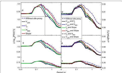
varia-tions of τ, φ and σ versus period are displayed in Fig. 5 for
all ANN models: without SCPs, one SCP and two SCPs.
Figure 5 shows that the between-event variability (τ) is
much lower than the within-event variability (φ), which is consistent with the vast majority of previous GMPE models results. The total variability (σ) is found identi-cal at very short period (T < 0.05 s) whatever the ANN model: none of the SCP is really efficient at high fre-quency. The various variability components then increase from 0.05 to about 0.15 s and then decrease significantly as period is increasing. A peak around 0.1 s has already been observed by some NGA-West2 GMPEs
develop-ers (e.g. Chiou and Youngs 2014; Derras et al. 2016). A
possible explanation is the interaction of varying stress drop with the high-frequency damping term (kappa). At short-to-intermediate periods, i.e. for T between 0.1 and 0.6 s, one-SCP models allow reducing the within-event standard deviation compared to the reference model.
The smallest φ is obtained for the VS30 SCP, followed by
f0 and H800 proxies, which have comparable performance,
while the slope proxy exhibits the poorest performance.
At longer periods, f0 and H800 provide the lowest φ values
and perform better than VS30.
As expected, the two-SCP models lead to larger vari-ance reductions, but it is interesting to notice than all pairs of proxies exhibit very similar performance. At short-to-intermediate periods, i.e. from 0.4 to 0.8 s, the
[VS30, f0] pair is found to provide the smallest values of φ,
while for T > 0.8 s the “best” pair turns out to be [f0, H800]
as logically expected since both parameters are more
sen-sitive to the bedrock depth. Interestingly enough, the [f0,
slope] pair exhibits a relatively good performance over the whole period range [0.1–4 s], while it is associated with the lowest measurement cost.
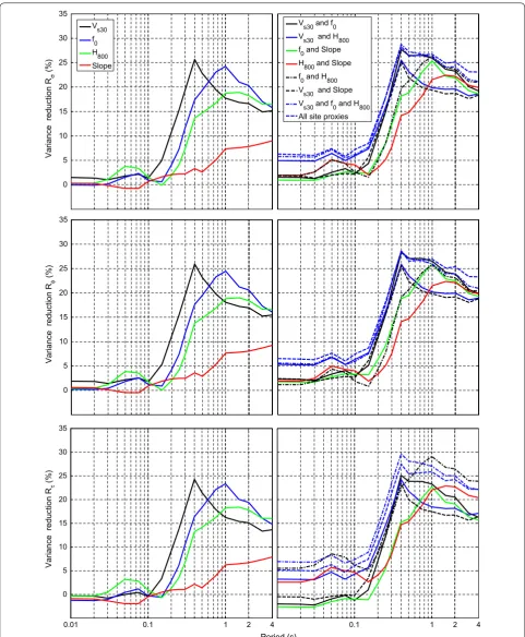
In addition, to better quantify the gains achieved by each SCP (s) model, the values of the variance reduction
coefficients Rσ, Rφ and Rτ defined in Eq. 2 are presented in
Fig. 6. The variations of these coefficients versus period
are displayed in Fig. 6 for all ANN models: without SCPs,
one-SCP, two-SCP, the best three-SCP model and the single four-SCP models. The reason for which we add these three and four SCPs cases is to obtain an estimate of the maximum possible variance reduction when many
site parameters are known. The Rσ values are also listed
in Table 3 for a limited set of ground-motion parameters
(PGA, PGV and PSA at T = [0.2, 0.5, 1.0, 2.0] s).
Fig. 4 Structure of the neural networks for PGA, PGV and PSA [0.01 to 4 s] prediction, for one site proxy (top) and two site proxies (bottom). The wh
ij is the synaptic weight between the ith neuron of the input
layer and the jth neuron in the hidden layer, bh
j the bias of the jth neu‑ ron in the hidden layer. Also the w0
jk is the synaptic weight between the jth neuron of the hidden layer and the kth neuron in the output layer, b0
The obtained results confirm that the reduction in the
aleatory variability becomes significant beyond T = 0.1 s
and for PGV as well (Table 3). For the short periods [0.1–
0.6 s], the best is VS30—with a maximum of 25% variance
reduction at 0.4 s—while f0 outperform in the [0.6, 4] s.
The variance reduction obtained with the slope SCP is the lowest of all SCPs (except between 0.1 and 0.2 s) and
reaches a maximum of 9% at 4 s. VS30 is thus confirmed
to be relevant mainly for short-to-intermediate periods, as expected from the fact that it samples only the
shal-low subsurface, while f0 and H800 are more sensitive to
the deep sediments and more relevant for long periods. Similarly, the “two-SCP” models exhibit a slightly larger variance reduction at short-to-intermediate period when
they include VS30 as one of the two site proxies (the best
(2)
performance being achieved by the [VS30, f0] pair), while
the largest reduction at long periods is observed for the
[f0, H800] pair, i.e. a combination of two long-period
prox-ies, with a value of Rσ reaching 24% at T = 2.0 s.
Over-all, the largest reduction is observed for the “reference” model accounting simultaneously for the four SCPs, fol-lowed by the three best SCPs model combining the use
of [VS30, f0, H800]; it is noteworthy, however, that such
“maximum possible” variance reduction does not exceed
1.5% for PGA (Table 3) and 4% for short periods around
0.08 s, while it reaches 29% around 0.4 s. The values of these variance reduction coefficients confirm that no site proxy can be preferred over the whole frequency range.
It is worth noticing in Figs. 5 and 6 that site proxies
also influence the between-event standard deviation τ in a very similar way they affect the within-event variabil-ity: it could be interpreted as resulting from the fact that a better site description enables a better description of the actual dependence of the dependence on the source and path parameters. It may also indicate that despite the random-effect procedure, the within- and between-event variabilities are not completely independent. Such 0.25
Fig. 5 Sensitivity of the aleatory variability components (total σ, within‑event, φ between‑event, τ) to the site proxies used as input for the neural network. The left frame corresponds to use one SCP as input. In right part, it is for two SCPs. The σ, φ, τ standard deviation values are provided both on log10 scale (left axis) and on ln scale (right axis). They are provided for spectral ordinates for periods from 0.01 to 4 s. The Mw and RJB are used to
0 5 10 15 20 25 30 35
Variance reduction
Rσ
(%)
Vs30 and f0 Vs30 and H800 f0 and Slope H800 and Slope f0 and H800 Vs30 and Slope Vs30 and f0 and H800 All site proxies Vs30
f0 H800 Slope
0 5 10 15 20 25 30 35
Variance reduction
Rφ
(%)
0.01 0.1 1 2 4
0 5 10 15 20 25 30 35
Variance reduction
Rτ
(%)
0.1 1 2 4
Period (s)
Fig. 6 Performance of various SCPs in reducing ground‑motion aleatory variability. The top frames display the variance coefficient reduction (Rσ)
for the total standard deviation σ. The middle frames illustrate the variance coefficient reduction (Rφ) of the within‑event standard deviation φ. The
bottom frames show the variance coefficient reduction (Rτ) of the between‑event standard deviation τ. In the left frames (for top, middle and bot‑
tom frames), we use four ANN models with one SCP measured VS30 or f0, H800 and slope. In the right frames (for top, middle and bottom frames), we
Table
or the 12 ANN mo
dependency with a slight trade-off between source- and site-related residuals has already been observed and
can-not be avoided (e.g. Ktenidou et al. 2017).
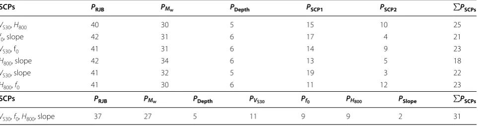
Another parameter used in ANN approach to measure the relevancy of each explanatory variable (and therefore of each single SCP or SCP pair) is the total percentage of
synaptic weights P. As explained in Derras et al. (2012) and
Derras et al. (2014), these synaptic weights P can be
esti-mated from the weights allocated to each input variable in each connection to the hidden layer and provide a meas-ure of the relative, overall importance of the individual explanatory variables, averaged for all the output ground-motion parameters (thus, here, over the whole frequency range 0.01–4 s). They have been computed according to
the procedure detailed in Derras et al. (2014, Equation 4),
for the 11 ANN models. Tables 4 and 5 list the P values
(in %) for each input variable. As expected from the data distribution, the most efficient parameter in reducing the
variance of response spectra is the RJB distance (synaptic
weight around 40–51%), followed directly by the
earth-quake magnitude Mw (around 27–36%). The P values
asso-ciated with the site term range from 7 to 31%. However,
focal depth does not have a great importance (PDepth ≅ 6).
When only one SCP is considered, the largest
SCP weights correspond to VS30 (around 19%) and
H800(≅ 18%), while the smallest corresponds to the slope
(Pslope = 7%). For the twin-SCP models, the best pair is
(VS30, H800) with P = 25%. The [f0, slope] pair also
per-forms well with P = 21%. This ranking is similar to the
ranking obtained from the analysis of aleatory vari-abilities discussed above if we consider the whole period range.
As in the aleatory variability analysis described above, the “all proxies” model is considered for comparison. The total synaptic weight of SCPs reaches 31%, which decom-poses in individual synaptic weights for each SCP rank-ing as for the synaptic weight of one-SCP models: the
largest one is PVS30, followed by Pf0 and PH800, the poorest
one is associated with the slope (PSlope = 3%). When the
number of SCP increases, the increase in the SCP weight is associated first with a decrease in the magnitude and
RJB weights (from one SCP to two SCPs), while the
rela-tive importance of the focal depth (from two SCPs to four SCPs) is 5–6%: the importance of focal depth is not
affected by the site described, while RJB and Mw obviously
remain key parameters.
Impact of the various SCPs on median ground‑motion models
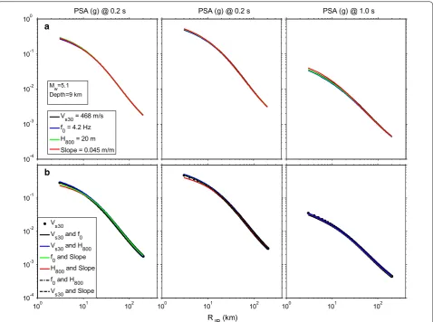
As discussed above, the nature of SCP has a notice-able effect on the ground-motion aleatory variability. We investigate here their impact on the median esti-mates, through a comparison of the four one-SCP ANN
and six two-SCP ANN models. Figure 7 displays the
dis-tance dependence of the spectral acceleration for T = 0.0,
0.2 and 1.0 s, for the median magnitude (Mw = 5.1),
the median focal depth (9 km), and the median values
of the various SCPs (i.e. VS30 = 468 m/s, f0 = 4.2 Hz,
H800 = 20 m and slope = 0.045 m/m, as derived from
Fig. 2 and Table 2). Through Fig. 7a, we remark that the
site proxy type (VS30/f0/H800/slope) is observed not to
have any significant impact on median predictions.
The two-SCP models (Fig. 7b) lead to similar results. All
pairs of proxies exhibit very similar median predictions, Table 4 Sensitivity of ground-motion models to
mag-nitude, distance and one SCP, as expressed through the
total percentages of synaptic weight (P, %) corresponding
to each input parameter
Table 5 Sensitivity of ground-motion models to magnitude, distance, depth, two SCPs and three SCPs, as expressed
through the total percentages of synaptic weight (P, %) corresponding to each input parameter
especially at short periods (T = 0.0 s, T = 0.2 s and
T = 1.0 s). Furthermore, the comparison with the VS30
-SCP model highlights the fact that the type and the number (one SCP or two SCPs) of site proxies have no influence on this median.
Ground motions for “Extreme” values of site proxies
Complementary information is provided by the amount of difference in predictions for “extreme” values of the
SCP. Figures 8 and 9 display the “soft/stiff” spectral ratio
(SR) for various periods (T = 0.0, 0.2 and 1.0 s): a
consist-ent definition of “soft” and “stiff” sites was taken for all SCPs, simply by considering the SCP values correspond-ing to 10 and 90% of the CDF distributions shown in
Fig. 2 and listed in Table 2; note, however, that given the
negative correlation between H800 and other proxies, the
10% fractile of H800 (i.e. 4 m) has been associated with the
90% fractile of VS30, f0 and slope (i.e. 829 m/s, 11.71 Hz
and 0.117 m/m, respectively), and vice versa (i.e. 86 m,
289 m/s, 0.66 Hz and 0.015 m/m, respectively). Figures 8
and 9 display such SR for individual SCP (top) and
two-SCP (bottom) cases. SR has the following form:
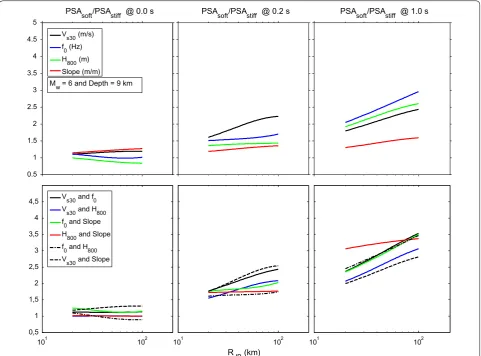
Figure 8 shows the sensitivity of the SR amplification
factors to RJB distance, at three different spectral
peri-ods (0.0, 0.2 and 1 s), and for a given earthquake scenario
(Mw = 6, depth = 9 km). Besides the trend of site
ampli-fication to increase with distance up to 100 km—which is related to nonlinear site response as the loading level is decreasing with increasing distance—the site ampli-fication is found to increase with period, as classically found in most GMPEs. The curves are displayed between
(3)
SR(T)= PSAsoft(T)
PSAStiff(T)
PSA (g) @ 0.2 s PSA (g) @ 1.0 s
10-4 10-3 10-2 10-1
100 PSA (g) @ 0.2 s
Vs30 = 468 m/s f0 = 4.2 Hz H800 = 20 m Slope = 0.045 m/m a
Mw=5.1
Depth=9 km
100 101 102
10-4 10-3 10-2 10-1
100 101 102
RJB (km)
100 101 102
Vs30 Vs30 and f0 Vs30 and H800 f0 and Slope H800 and Slope f0 and H800 Vs30 and Slope b
Fig. 7 Median ground motion predicted by different models. Effect of the one‑SCP proxy (top, VS30/f0/H800/slope) and the two SCPs in the bottom row. The plots display the distance dependence of the spectral accelerations at three periods (T= 0.0 s, left column; T= 0.2 s, middle column; and
[20 and 100] km, considered reliable, since the derived models can hardly be considered reliable for soft and stiff sites at lower distances to 20 km or greater than 100 km
(see Fig. 1). VS30 and slope SCPs are found to provide
the amplification at short periods (which remains, how-ever, smaller than 27%). The situation is opposite at long
period (T = 1.0 s) where the SCP providing the largest
amplification is f0 with amplification ranging from 2 to 3.
In addition, it is clear that the site amplification predicted with the slope proxy is not very sensitive to the oscillator period. Another interesting result is that the combination of two proxies significantly increases the “soft/stiff” SR
values: the amplification increase ranges from 3% (VS30 to
VS30–slope) at short period, to 12% at intermediate
peri-ods, to 16% at long period (f0 to f0–VS30). The most
prob-able explanation comes from the fact that simultaneously matching 10 and 90% fractiles for a pair of proxies cor-responds to less frequent combinations, with more differ-entiated site conditions, than for a single proxy (as also
shown in Fig. 3).
Figure 9 illustrates the SR amplification factors
varia-tion versus PSAstiff at T = 0.0 s (i.e. PGAstiff), one of the
reference parameters that is commonly used in GMPEs to describe the dependence of the nonlinear site amplifi-cation on the loading level. These curves have been
estab-lished here by considering a given RJB distance (30 km), a
given focal depth (9 km) and a magnitude varying from 5 to 7 with an equal increment 0.125. A closer look at the dependence of soft/stiff amplification factor does indicate a larger amplification level for small stiff motion levels, associated with a significant nonlinearity (i.e. decrease in amplification with increasing loading level at the
under-lying bedrock). The curves displayed in Fig. 9 call for
sev-eral comments:
1. The amount of nonlinearity depends both on the considered site proxies and on the oscillator period. 2. Whatever the site proxy, a significant nonlinearity
3. Among single proxy models, the one using the slope predicts similar nonlinearity whatever the oscillator
period, while the “long-period” proxies f0 and H800
are those who do not predict any significant nonlin-earity at short period: the predicted SR is around 1
at T = 0.0 s and around 1.8 to 1.5 at T = 0.2 s. At
long period (T = 1.0 s), the SCP providing the
larg-est SR is f0, while amplification levels and their
non-linear sensitivity on PGAstiff are almost similar to
VS30 and H800 proxies. This larger amplification
fac-tors for the f0 model at T = 1.0 s might be related to
the fact that the “soft” site is characterised by a fun-damental frequency of 0.66 Hz: the oscillator fre-quency (1 Hz) is always larger than the fundamental frequency, and one may thus expect to be system-atically in the amplified frequency range, while sites
with VS30 = 289 m/s or H800 = 86 m, with
funda-mental frequencies above 1 Hz (see the last column
of Fig. 3), do exist. Correlatively, a larger reduction in
the amplification with increasing loading level may be expected if the nonlinear behaviour affects the whole thickness of the soil deposit (see Régnier et al. 2016).
4. Similar observations can be done for the results
with two-SCP models. At short period (T = 0 and
0.2 s), the largest amplification and nonlinearity are predicted when using the pair of short-period
prox-ies (VS30–slope and VS30–f0), while the smallest
cor-responds to the pair of long-period proxies (f0–H800
and H800–slope). At long period (T = 1.0 s), the
pre-dicted amplifications and their nonlinear component are less scattered than in the one-SCP case, the pairs
including the f0 proxy predicting, however, slightly
larger amplifications. 0.5
1 1.5 2 2.5 3 3.5 4 4.5
5 PSAsoft/PSAstiff @ 0.0 s
RJB=30 km; Depth=9 km
Mw=[5 to 7]
PSAsoft/PSAstiff @ 0.2 s PSAsoft/PSAstiff @ 1.0 s
Vs30 (m/s) f0 (Hz) H800 (m) Slope (m/m)
10-2 10-1
0.5 1 1.5 2 2.5 3 3.5 4 4.5
10-2 10-1
PSAstiff (g) @ 0.0 s
10-2 10-1
Vs30 and f0 Vs30 and H800 f0 and Slope H800 and Slope f0 and H800 Vs30 and Slope
Fig. 9 Illustration of the nonlinearity in the site term. Site amplification factor (SR: Eq. 3) versus PGArstiff (90% of CDF) at T= 0.0, 0.2, 1.0 s for
These results are, however, partial and should not be extrapolated too fast, as they correspond to a specific distance (and focal depth) and use the stiff-site PGA to characterise the loading level.
Figures 10, 11, 12 and 13 are thus intended to check
the robustness of the results presented in Fig. 9,
con-sidering also other descriptions of the loading level and other distance scenario. Only one-SCP models are
con-sidered, successively VS30, f0, H800 and slope for Figs. 10,
11, 12 and 13, respectively. In each case, three different
distances are considered (30, 50 and 75 km) i.e. in the range where there exist enough data within the [10–90%] fractile range of each SCP, and the variation of the load-ing level for each distance corresponds to the predictions over the magnitude range [5–7] with an equal increment of 0.125. Three different parameters are considered to characterise the loading level: the PGA on rock or “stiff” site as defined according to the selected site proxy, the spectral acceleration on the same rock or “stiff” site at the oscillator period considered, and finally an estimate of the actual strain at the site: several authors (Idriss,
2011; Chandra et al. 2015, 2016; Guéguen 2016)
pro-posed to use the ratio PGV/VS30 as a proxy to the shear
strain, where PGV is the peak velocity at the site, and it has thus been tested in the present study. In principle, if a loading parameter is relevant for nonlinear behav-iour, the dependency of site amplification as a function of this loading parameter should exhibit only a marginal dependency on other parameters such as magnitude, or
distance or frequency contents. Analysing Figs. 10, 11, 12
and 13 according to this criterion clearly indicates that
the lowest scatter is observed among distance and
mag-nitude scenarios for the loading parameter “PSAstiff(T)”
(second row), while the largest corresponds to “PGAstiff”,
especially for the long-period site amplification.
In the light of these results, it turns out that the best ground-motion parameter to be used for the characteri-sation of the loading level in the nonlinear site amplifica-tion term of GMPEs is the spectral ordinate on rock at
the considered period; the strain proxy PGV/VS30 may,
however, constitute a satisfactory, alternative choice. Another major outcome of this section is the variability of the nonlinear behaviour according to the site proxy selected for the GMPEs: short-period nonlinearity is
observed preferably with short-period proxies (VS30 and
slope) and disappears when using H800.
Summary and conclusions
The application of neural networks approach to a KiK-net data set offered the possibility to test the performance of various site-condition proxies to reduce the aleatory
variability in GMPEs. The four available SCPs are VS30
and H800 (both derived from downhole measurements),
f0 (the fundamental frequency derived from H/V ratios
and surface/downhole spectral ratios), and the slope derived from DEM data, which has been proposed as a
proxy to VS30 values. A total of 16 neural network
mod-els were derived to describe the dependence of response
spectra ordinates on moment magnitude Mw, Joyner and
Boore distance RJB, focal depth and various combinations
of SCPs: one without any SCP which provides the “ref-erence case”, four with each single SCP, six with the six
possible pairs of SCPs [VS30–f0], [VS30–H800], [f0–slope],
[H800–slope], [VS30–slope] and [f0–H800], four with the four possible combinations of three SCPs, and one will all SCPs considered simultaneously.
When only one SCP is used, the largest reduction in aleatory variability with respect to the “reference case”
is found to be provided by VS30 at short-to-intermediate
periods (T ≤ 0.6 s), and by f0 or H800 at longer periods.
Among the four SCPs, the parameter “slope” is thus found to provide the worst performance when consid-ered alone. However, when SCP pairs are considconsid-ered, comparable performance is found whatever the pair of proxies. In particular, the “best pairs” are found to be
[VS30–H800] at short periods and [f0–H800] at long
peri-ods, while the “low-cost” pair [f0–slope] provides a good
compromise over the whole period range [0.1–4 s]. None of the four tested SCPs is thus “optimal” over the whole period range, and all proxies show a poor contribution at high frequencies (>10 Hz).
Otherwise, the site proxy type (slope/VS30/H800/f0) has
no influence on the median, and these results indicate that the type of SCP does not really affect the median.
Regarding site amplification, VS30 and slope SCPs are
found to provide some differentiation at short periods
(0, 0.2 s). At long period, H800 and f0 are providing the
largest differentiation. We showed also that, for this sub-set of KiK-net data, the soft-to-stiff-site amplifications exhibit a significant nonlinearity, the characteristics of which are, however, tightly linked to the used proxy, and the parameter selected to describe the loading level. The most relevant loading parameter is found to be the spec-tral acceleration on rock (or “stiff” site) at the considered period, and the worst the rock (or “stiff”) peak accelera-tion, with a satisfactory behaviour for the strain proxy
PGV/VS30. Nonlinearities are found to be systematically
larger at intermediate period (1 s) than at short period (0.2, 0 s). This purely data-driven result is rather intrigu-ing and calls for further checks, such as the use of larger data sets, especially at long periods (for instance, adding recordings from interplate earthquakes), the compari-son with the site-specific nonlinearities as defined by the
RSRNL-L ratio introduced by Régnier et al. (2013, 2016),
10-3 10-2 10-1 0.5
1 1,5 2 2,5 3 3.5
4 PSAsoft/PSAstiff @ 0.0 s
10-3 10-2 10-1
PGVsoft/Vs30 (%) PSAsoft/PSAstiff @ 0.2 s
10-3 10-2 10-1
PSAsoft/PSAstiff @ 1.0 s
30 km 50 km 75 km Vs30 site proxy
Mw=[5-7], depth=9 km
10-2 10-1
0.5 1 1.5 2 2.5 3 3.5 4
PSAstiff @ 0.0 s
10-2 10-1
PSAstiff @ 0.2 s
10-2 10-1
PSAstiff @ 1.0 s
10-2 10-1
0.5 1 1.5 2 2.5 3 3.5 4
10-2 10-1
PSAstiff (g) @ 0.0 s
10-2 10-1
Fig. 10 Comparison of the NL components of site amplification for different descriptions of the loading level, for the one‑SCP ANN model using
derived only for weak motions, and possibly the testing
of other, basin-related, site proxies such as H1100 or H2500.
Another important result (which will also have to be investigated further) is the variability of the nonlinear
site response according to the SCP: short-period non-linearity is observed preferably with short-period
proxies (VS30 and slope) and disappears when using
H800.
10-3 10-2 10-1
0.5 1 1,5 2 2,5 3 3.5 4
PSAsoft/PSAstiff @ 0.0 s
10-3 10-2 10-1
PGVsoft/Vs30 (%) PSAsoft/PSAstiff @ 0.2 s
10-3 10-2 10-1
PSAsoft/PSAstiff @ 1.0 s
30 km 50 km 75 km Mw=[5-7], depth=9 km f0 site proxy
10-2 10-1
0.5 1 1.5 2 2.5 3 3.5 4
PSAstiff @ 0.0 s
10-2 10-1
PSAstiff @ 0.2 s
10-2 10-1
PSAstiff @ 1.0 s
10-2 10-1
0.5 1 1.5 2 2.5 3 3.5 4
10-2 10-1
10-2 10-1
PSAstiff (g) @ 0.0 s
Fig. 11 Similar to Fig. 10, but for the one‑SCP model—using f0 as site‑condition proxy. Stiff site corresponds to f0= 11.71 Hz, soft site to
10-3 10-2 10-1 0.5
1 1,5 2 2,5 3 3.5 4
PSAsoft/PSAstiff @ 0.0 s
10-3 10-2 10-1
PGVsoft/Vs30 (%) PSAsoft/PSAstiff @ 0.2 s
10-3 10-2 10-1
PSAsoft/PSAstiff @ 1.0 s
30 km 50 km 75 km Mw=[5-7], depth=9 km H800 site proxy
10-2 10-1
0.5 1 1.5 2 2.5 3 3.5 4
PSAstiff @ 0.0 s
10-2 10-1
PSAstiff @ 0.2 s
10-2 10-1
PSAstiff @ 1.0 s
10-2 10-1
0.5 1 1.5 2 2.5 3 3.5 4
10-2 10-1
10-2 10-1
PSAstiff (g) @ 0.0 s
Fig. 12 Similar to Fig. 10, but for the one‑SCP model—using H800 as site‑condition proxy. Stiff site corresponds to H800= 4 m, soft site to
10-3 10-2 10-1 0.5
1 1,5 2 2,5 3 3.5 4
PSAsoft/PSAstiff @ 0.0 s
10-3 10-2 10-1
PGVsoft/Vs30 (%) PSAsoft/PSAstiff @ 0.2 s
10-3 10-2 10-1
PSAsoft/PSAstiff @ 1.0 s
30 km 50 km 75 km Mw=[5-7], depth=9 km Slope site proxy
10-2 10-1
0.5 1 1.5 2 2.5 3 3.5 4
PSAstiff @ 0.0 s
10-2 10-1
PSAstiff @ 0.2 s
10-2 10-1
PSAstiff @ 1.0 s
10-2 10-1
0.5 1 1.5 2 2.5 3 3.5 4
10-2 10-1
10-2 10-1
PSAstiff (g) @ 0.0 s
As these results have been obtained on a specific— though large—data set (subset of KiK-net data, thus probably lacking of very soft sites), they should of course be tested for other data sets; the four SCPs are, however, rarely available simultaneously.
Abbreviations
SCP: site‑condition proxy; VS30: time-averaged shear-wave velocity in the top 30 m; H800: depth beyond which Vs exceeds 800 m/s; f0: fundamental reso‑ nance frequency; Slope: topographical slope; DEM: digital elevation models; PGA: peak ground acceleration; PGV: peak ground velocity; PSA: pseudo‑spec‑ tral acceleration; GMPEs: ground‑motion prediction equations; ANN: artificial neural network; Mw: moment magnitude; RJB: Joyner and Boore distance; Depth: focal depth; CDF: cumulative distribution function; R: coefficient of correlation; τ: between‑event standard deviation; φ: within‑event standard deviation; σ: total standard deviation; Rτ: between‑event variance reduction
coefficient; Rφ: within‑event variance reduction coefficient; Rσ: total variance
reduction coefficient; P: total percentage of synaptic weights; SR: spectral ratio.
Authors’ contributions
Most of the scientific and technical work has been carried out by BD, under the scientific supervision of P‑YB and FC. The redaction has been shared among the three authors. All authors read and approved the final manuscript.
Author details
1 Risk Assessment and Management Laboratory (RISAM), Abou Bekr Belkaïd University, BP 230, 13048, Chetouane, Tlemcen, Algeria. 2 Department of Civil Engineering and Hydraulics, Dr Moulay Tahar University, BP 138, 20000, Ennasr, Saïda, Algeria. 3 Institut des Sciences de la Terre (ISTerre), IFSTTAR, CNRS, IRD, Bâtiment OSUG C, Grenoble‑Alpes University, CS 40700, 38058 Grenoble Cedex 9, France. 4 Section 2.6 Hazard and Stress Field, GFZ German Research Center for Geoscience, Telegrafenberg, 14473 Potsdam, Germany. 5 Institute of Earth and Environmental, University of Potsdam, Potsdam, Germany.
Acknowledgements
The authors thank Julie Régnier and Héloïse Cadet for their generous help and which provided us the f0 of the KiK‑net database. We acknowledge the sup‑ port from the TASSILI program, the sinaps@ project (http://www.institut‑seism. fr/projets/sinaps/). We also thank an anonymous reviewer for their construc‑ tive criticism and comments that helped us to improve this study. The authors would like to thank Haitham Dawood and Adrian Rodriguez‑Marek for provid‑ ing high‑quality data.
Competing interests
The authors declare that they have no competing interests.
Data and resources
PSA, VS30 and H800 used in this study were collected from the KiK‑net website
https://datacenterhub.org/resources/272. Slope have been collected and disseminated by the “The Pacific Earthquake Engineering Research Center” at
http://peer.berkeley.edu/ngawest2/databases/. f0 from Régnier et al. (2013).
Publisher’s Note
Springer Nature remains neutral with regard to jurisdictional claims in pub‑ lished maps and institutional affiliations.
Received: 18 January 2017 Accepted: 11 September 2017
References
Abrahamson NA, Youngs RR (1992) A stable algorithm for regression analyses using the random‑effects model. Bull Seismol Soc Am 82(1):505–510 Akaike H (1973) Information theory and an extension of the maximum likeli‑
hood principle. In: Proceedings of the 2nd international symposium on information theory, vol 1, pp 267–281. Budapest, Hungary
Al Atik L, Abrahamson N, Bommer JJ, Scherbaum F, Cotton F, Kuehn N (2010) The variability of ground motion prediction models and its components. Seismol Res Lett 81(5):794–801
Allen TI, Wald DJ (2009) On the use of high‑resolution topographic data as a proxy for seismic site conditions (VS30). Bull Seismol Soc Am 99:935–943
Ancheta TD, Darragh RB, Stewart JP, Seyhan E, Silva WJ, Chiou S‑J, Wooddell KE, Graves RW, Kottke AR, Boore DM, Kishida T, Donahue JL (2014) NGA‑West 2 database. Earthq Spectra 30(3):989–1005
Bard P‑Y, Cadet H, Endrun B, Hobiger M, Renalier F, Theodulidis N, Ohrnberger M, Fäh D, Sabetta F, Teves‑Costa P, Duval A‑M, Cornou C, Guillier B, Wathelet M, Savvaidis A, Köhler A, Burjanek J, Poggi V, Gassner‑Stamm G, Havenith HB, Hailemikael S, Almeida J, Rodrigues I, Veludo I, Lacave C, Thomassin S, Kristekova M (2010) From non‑invasive site characterisation to site amplification: Recent advances in the use of ambient vibration measurements. In: Garevski M, Ansal A (eds) Earthquake engineering in Europe. Geotechnical, geological, and earthquake engineering books, New York, pp 105–123
Boore DM (2005) On pads and filters: processing strong‑motion data. Bull Seismol Soc Am 95(2):745–750
Boore DM, Joyner WB, Fumal TE (1993) Estimation of response spectra and peak accelerations from western North American earthquakes: an interim report, part 2. U.S. Geological Survey Open‑File Report 94‑127
Boore DM, Joyner WB, Fumal TE (1997) Equations for estimating horizontal response spectra and peak acceleration from western North American earthquakes: a summary of recent work. Seismol Res Lett 68(1):128–153 Borcherdt RD (1994) Estimates of site‑dependent response spectra for design
(methodology and justification). Earthq Spectra 10(4):617–653 Brillinger DR, Preisler HK (1985) Further analysis of the Joyner‑Boore attenua‑
tion data. Bull Seismol Soc Am 75:611–614
Cadet H, Bard P‑Y, Duval A‑M, Bertrand E (2011) Site effect assessment using KiK‑net data: part 2—site amplification prediction equation based on f0 and Vsz. Bull Earthq Eng 10(2):451–489
Campbell KW (1989) Empirical prediction of near‑source ground motion for the Diablo Canyon power plant site. San Luis Obispo County, California, U.S. Geological Survey Open‑File Report 89‑484
Campbell KW (1993) Empirical prediction of near‑source ground motion from large earthquakes. In: Proceedings international workshop on earthquake hazards and large dams in the Himalaya, January 15–16, New Delhi, India
Chandra J, Gueguen P, Steidl JH, Bonilla LF (2015) In‑situ assessment of the G‑γ curve for characterizing the nonlinear response of soil: application to the Garner Valley downhole array(GVDA) and the wildlife liquefaction array (WLA). Bull Seismol Soc Am 105(2A):993–1010
Chandra J, Gueguen P, Bonilla LF (2016) PGA‑PGV/Vs considered as a stress– strain proxy for predicting nonlinear soil response. Soil Dyn Earthq Eng 85:146–160
Chiou B‑SJ, Youngs RR (2008) An NGA model for the average horizontal com‑ ponent of peak ground motion and response spectra. Earthq Spectra 24(1):173–215
Chiou B‑SJ, Youngs RR (2014) Update of the Chiou and Youngs NGA ground motion model for average horizontal component of peak ground motion and response spectra. Earthq Spectra 30:1117–1153
Choi Y, Stewart JP (2005) Nonlinear site amplification as function of 30 m shear wave velocity. Earthq Spectra 21(1):1–30
Dawood HM, Rodriguez‑Marek A, Bayless J, Goulet C, Thompson E (2015) NEES: The KiK‑net database processed using an automated ground motion processing protocol. https://datacenterhub.org/resources/272
Dawood HM, Rodriguez‑Marek A, Bayless J, Goulet C, Thompson E (2016) A flatfile for the KiK‑net database processed using an automated protocol. Earthq Spectra 32(2):1281–1302
Demuth H, Beale M, Hagan M (2009) Neural Network Toolbox™6: user’s guide. MATLAB. The MathWorks Inc, Natick
Derras B, Bard P‑Y, Cotton F, Bekkouche A (2012) Adapting the neural network approach to PGA prediction: an example based on the KiK‑net data. Bull Seismol Soc Am 102(4):1446–1461
Derras B, Bard P‑Y, Cotton F (2014) Towards fully data‑driven ground‑motion prediction models for Europe. Bull Earthq Eng 12(1):495–516 Derras B, Bard P‑Y, Cotton F (2016) Site‑conditions proxies, ground‑motion
Guéguen P (2016) Predicting nonlinear site response using spectral accel‑ eration vs PGV/VS30: a case history using the Volvi‑test site. Pure appl Geophys 173(6):2047–2063
Haghshenas E, Bard P‑Y, Theodulidis N, SESAME WP04 Team (2008) Empirical evaluation of microtremor H/V spectral ratio. Bull Earthq Eng 6(1):75–108 Hayashida T, Tajima F (2007) Calibration of amplification factors using KiK‑net
strong‑motion records: toward site effective estimation of seismic intensi‑ ties. Earth Planets Space 59:1111–1125. doi:10.1186/BF03352054
Idriss IM (2011) Use of VS30 to represent local site condition. In: Proceedings of the 4th IASPEI/IAEE international symposium. Effects of source geology on seismic motion, August 23–26, California, USA
Ktenidou O‑J, Roumelioti Z, Abrahamson N, Cotton F, Pitilakis K, Hollender F (2017) Understanding single‑station ground motion variability and uncertainty (sigma): lessons learnt from EUROSEISTEST. Bull Earthq Eng. doi:10.1007/s10518‑017‑0098‑6
Luzi L, Puglia R, Pacor F, Gallipoli MR, Bindi D, Mucciarelli M (2011) Proposal for a soil classification based on parameters alternative or complementary to Vs, 30. Bull Earthq Eng 9(6):1877–1898
Mucciarelli M (1998) Reliability and applicability of Nakamura’s tech‑ nique using microtremors: an experimental approach. J Earthq Eng 2(04):625–638
Régnier JH, Cadet LF, Bonilla LF, Bertrand E, Semblat J‑F (2013) Assessing nonlinear behavior of soils in seismic site response: statistical analysis on KiK‑net strong‑motion data. Bull Seismol Soc Am 103(3):1750–1770 Régnier J, Cadet H, Bard P‑Y (2016) Empirical quantification of the impact
of non‑linear soil behaviour on site response. Bull Seismol Soc Am 106(4):1710–1719
Sadigh K, Chang C‑Y, Egan JA, Makdisi FI, Youngs RR (1997) Attenuation relationships for shallow crustal earthquakes based on California strong motion data. Seismol Res Lett 68(1):180–189
Seyhan E, Stewart JP, Ancheta TD, Darragh RB, Graves RW (2014) NGA‑West2 site database. Earthq Spectra 30(3):1007–1024
Shanno DF, Kettler PC (1970) Optimal conditioning of quasi‑Newton methods. Math Comput 24:657–664