Nonlinear Multiantenna Detection Methods

(1)

Nonlinear Multiantenna Detection Methods

Sheng Chen

School of Electronics and Computer Science, University of Southampton, Southampton SO17 1BJ, UK Email:[email protected]

Lajos Hanzo

Andreas Wolfgang

Received 29 May 2003; Revised 16 February 2004

A nonlinear detection technique designed for multiple-antenna assisted receivers employed in space-division multiple-access sys-tems is investigated. We derive the optimal solution of the nonlinear spatial-processing assisted receiver for binary phase shift keying signalling, which we refer to as the Bayesian detector. It is shown that this optimal Bayesian receiver significantly out-performs the standard linear beamforming assisted receiver in terms of a reduced bit error rate, at the expense of an increased complexity, while the achievable system capacity is substantially enhanced with the advent of employing nonlinear detection. Specifically, when the spatial separation expressed in terms of the angle of arrival between the desired and interfering signals is below a certain threshold, a linear beamformer would fail to separate them, while a nonlinear detection assisted receiver is still capable of performing adequately. The adaptive implementation of the optimal Bayesian detector can be realized using a radial basis function network. Two techniques are presented for constructing block-data-based adaptive nonlinear multiple-antenna as-sisted receivers. One of them is based on the relevance vector machine invoked for classification, while the other on the orthogonal forward selection procedure combined with the Fisher ratio class-separability measure. A recursive sample-by-sample adaptation procedure is also proposed for training nonlinear detectors based on an amalgam of enhancedκ-means clustering techniques and the recursive least squares algorithm.

Keywords and phrases:smart antenna, adaptive beamforming, mean square error, bit error rate, Bayesian classification, radial basis function network.

1. INTRODUCTION

Spatial processing invoking adaptive antenna arrays has shown real promise in terms of attaining substantial capacity enhancements in mobile communication [1,2,3,4,5,6,7, 8]. Multiple-antenna aided receivers are capable of separating signals transmitted on the same carrier frequency, provided that signals are su_fficiently separated in the spatial domain. Classically, beamforming algorithms create a linear combi-nation of the signals received from the di_fferent elements of an antenna array. We refer to this classic beamforming prin-ciple aslinearbeamforming. A traditional approach to lin-ear beamforming is based on the minimum mean square er-ror (MMSE) principle that minimizes the mean square erer-ror (MSE) between the desired output generated from a known reference signal and the actual array output. Adaptive imple-mentations of the linear MMSE (LMMSE) beamforming

so-lution can readily be realized using the well-known family of temporal reference techniques [2,3,9,10,11,12,13]. Specif-ically, block-data-based beamformer weight adaptation can be achieved using the sample matrix inversion (SMI) algo-rithm [9,10], while sample-by-sample based array-weight adaptation can be carried out using the least mean square (LMS) algorithm [11,12,13]. Recent work [14,15] has in-vestigated a linear beamforming technique based directly on minimizing the system’s bit error rate (BER) rather than the MSE and developed both block-data-based and sample-by-sample adaptive algorithms for implementing linear mini-mum BER (LMBER) beamforming. The results of [14,15] have demonstrated that LMBER beamforming is capable of providing considerable performance gains in terms of a re-duced BER over the usual LMMSE beamforming.

(2)

ˆ

b1(k)

R

ec

ei

ve

r

x1(t)

x2(t)

xL(t)

n1(t)

n2(t)

nL(t) P

P

P . . . .

. .

Modulator

b1(k)

b2(k)

bM(k) User 1

User 2

UserM

Desired

Interfering

Figure_{1: Multiantenna receiver configuration for the multiuser space-division multiple-access system.}

signal and the closest interfering signal dominates the achiev-able system performance and hence the system’s user capac-ity. When this angular separation is below a certain thresh-old, linear beamforming ultimately fails since the signals transmitted by the individual users become linearly insep-arable, a situation that has also been observed in the con-text of single-user channel equalization and multiuser de-tection designed for code-division multiple access (CDMA) [16,17,18,19,20]. In fact, it has been observed even in lin-early separable scenarios that a nonlinear processing tech-nique is capable of providing a better performance than a linear one, although this is typically achieved at the cost of an increased complexity. In conjunction with nonlinear spa-tial processing, the achievable system capacity can be signifi-cantly increased since an adequate performance can be main-tained even in case of a low angular separation compared to linear beamforming. These considerations motivate this study of nonlinear detection techniques contrived for multi-antenna aided systems.

The outline of the paper is as follows.Section 2 intro-duces the system model, while Section 3 outlines our lin-ear beamforming-based benchmarker. InSection 4, we de-rive the optimal solution of the nonlinear spatial processing assisted receiver for binary phase shift keying (BPSK) sig-nalling, which is referred to as the Bayesian detection solu-tion. It is shown that this Bayesian solution has an identi-cal form to a radial basis function (RBF) network [17,21]. InSection 5, two schemes are proposed for realizing block-data-based adaptive RBF detectors. One of them is based on the relevance vector machine (RVM) invoked for clas-sification [22,23] and the other one is the orthogonal for-ward selection (OFS) procedure using the Fisher ratio class-separability measure [24]. Finally, inSection 6, an adaptive sample-by-sample implementation of the RBF detector is also considered using an amalgam of the enhancedκ-means clustering and the recursive least squares (CRLS) algorithm [19,25] before offering our conclusions inSection 7.

2. SYSTEM MODEL

We consider the multiple-antenna aided receiver configura-tion ofFigure 1invoked for assisting the operation of a mul-tiuser SDMA system. It is assumed that the system supports

M users (signal sources), and each user transmits a BPSK modulated signal on the same carrier frequency ofω=2π f. Letk denote the bit instance. Then the baseband signal of useri, sampled at symbol rate, is given by

mi(k)=Aibi(k), 1≤i≤M, (1)

where the complex-valued coe_fficientAimodels the

multipli-cation of the channel coe_fficient of useriwith the transmitted signal power of useriand therefore|Ai|2denotes the received

signal power for useri, andbi(k)∈ {±1}is thekth bit of user i. Without any loss of generality, source 1 is assumed to be the desired user and the rest of the sources are the interfering users. A linear antenna array is considered which consists of

Luniformly spaced elements, and the signals received by the

L-element antenna array are given by

xl(k)= M

X

i=1

mi(k) exp¡jωtl¡θi¢¢+nl(k)=x¯l(k) +nl(k) (2)

for 1 ≤ l ≤ L, where tl(θi) is the relative time delay

at element l for sourcei, θi is the direction of arrival for

sourcei, andnl(k) is a complex-valued white Gaussian noise

with zero mean andE[|nl(k)|2] = 2σn2. The desired user’s

signal-to-noise ratio is defined as SNR = |A1|2/2σn2, and

the desired signal-to-interference ratio with respect to in-terfering user i is defined by SIRi = |A1|2/|Ai|2 for i =

2,. . .,M. In vectorial form, the antenna array outputx(k)= [x1(k) x2(k) · · · xL(k)]Tcan be expressed as

x(k)=x(¯ k) +n(k)=Pb(k) +n(k), (3)

wheren(k) =[n1(k) n2(k) · · · nL(k)]T has a covariance

matrix ofE[n(k)nH₍_k_)]₌₂_σ2

(3)

identity matrix, the system matrixPis given by

P=hA1s1 A2s2 · · · AMsM

i

, (4)

the steering vector for sourceiis formulated as

si= and the transmitted bit vector is

b(k)=hb1(k) b2(k) · · · bM(k)

iT

. (6)

The task of the spatial-processing assisted receiver is to provide an estimate ˆb1(k) of the desired user’s

transmit-ted bit b1(k), given the input x(k). To keep our notations

and the associated concepts relatively simple, we have used a BPSK modulation scheme, a narrowband channel model, and narrowband beamforming (space-only processing). The approach can be extended to other modulation schemes and wideband channels that induce intersymbol interference. The same idea can also be applied to broadband beamform-ing (space-time processbeamform-ing).

3. LINEAR BEAMFORMING ASSISTED RECEIVER

The output of the linear beamformer is given by

y(k)=wH_x(_k₎₌_wH_x(_¯ _k_{) +}_wH_n(_k₎₌_y_¯₍_k_{) +}_e₍_k_), ₍₇₎

wherew=[w1 w2 · · · wL]Tis the complex-valued

beam-former weight vector, ande(k) is Gaussian distributed with a zero mean and a varianceE[|e(k)|2_]₌₂_σ2

cally, the linear beamformer’s weight vector is determined by minimizing the MSE term ofE[|b1(k)−y(k)|2] between the

desired user’s transmitted bit and the beamformer’s output, which leads to the following LMMSE solution:

wMMSE=¡PPH+ 2σn2IL¢−1p1 (9)

withp1being the first column ofP. Using a temporal

refer-ence technique aided approach [7], the LMMSE beamform-ing solution can be readily realized usbeamform-ing the block-data-based SMI algorithm [7], and recursive sample-by-sample adaptation can be performed using the LMS or RLS algo-rithm [21].

In order to derive the BER formula of the linear beam-former with the weight vectorw, firstly note that there are

Nb = 2M possible sequences ofb(k), which are denoted as

bq, 1≤q≤Nb. Furthermore, denote the first element ofbq,

corresponding to the desired user, asbq,1. As expected, the

noiseless part of the beamformer input signal, ¯x(k), assumes encountering values only from the signal set defined as

X,© ¯

xq=Pbq, 1≤q≤Nbª. (10)

This set can be partitioned into two subsets depending on the specific value ofb1(k) as follows:

X(±),© ¯

xq(±)∈X:b1(k)= ±1ª. (11)

Similarly, ¯y(k) takes values from the scalar set

Y,© ¯

yq=wHx¯q, 1≤q≤Nbª (12)

which can be divided into the two subsets defined as

Y(±)_,©

which can be partitioned into the two subsets conditioned on the value ofb1(k):

Y(R±),

© ¯

yR(±,q)∈YR:b1(k)= ±1ª. (15)

It can be readily seen that the conditional probability density function (pdf) ofy(k) givenb1(k) = +1 is a

Gaus-sian mixture given by

p(y|+ 1)= 1

points inY(+)_{. Therefore, the conditional marginal pdf of}

yR(k) givenb1(k)=+1 is formulated as follows:

(4)

θ≤30◦

Interferer source 2 Desired

source 1

θ

Interferer source 3

45◦

30◦

Interferer source 4

λ/2

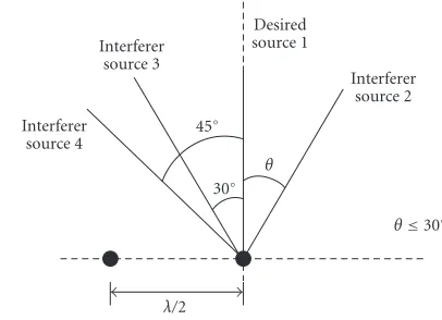
Figure _{2: Locations of the desired source and the interfering} sources with respect to the two-element linear antenna array hav-ingλ/2 element spacing, whereλis the wavelength.

The LMBER beamforming solution is then defined as fol-lows:

wMBER=arg min

w PE(w). (20)

Unlike the LMMSE solution (9), there exists no closed-form LMBER solution. In [14,15], a simplified conjugate gradient method [26,27] is used to obtain numerical solutions. Both the block-data-based gradient and LMS-style stochastic gra-dient adaptive algorithms have been derived in [14,15] to realize the LMBER beamforming solution.

For the linear beamformer to work adequately, the un-derlying system must be linearly separable. The linear separa-bility means that there exists a weight vectorwsuch thatY(R−)

andY(+)R are completely separated by the decision threshold yR = 0. When the minimum spatial separation expressed

in angles of arrival between the desired user and interfer-ing users is below a certain threshold, the system inevitably becomes linearly inseparable. In such a situation, the linear beamformer will have a high irreducible BER floor, and non-linear processing has to be adopted for the sake of achieving an adequate BER performance. In general, nonlinear spatial processing is capable of achieving a better performance than a linear receiver, regardless whether the output of the system is linearly separable or not. The limitation of a linear beam-forming assisted receiver is illustrated in the following exam-ple, which is also used throughout this paper for investigating the proposed nonlinear multiantenna detection techniques.

Simulation example

The example consisted of four signal sources and a two-element antenna array.Figure 2shows the locations of the desired source and the three interfering sources in a graphi-cal form. The simulated channel conditions wereAi=1 +j0,

1≤i≤4. The desired user and all the three interfering users had equal signal power, and therefore we had SIRi = 0 dB

fori=2, 3, 4. The minimum spatial separation in this exam-ple was the difference in angles of arrival between the desired user 1 and the interferer 2, which wasθ≤30◦_._{Figure 3}

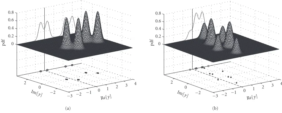
com-pares the BERs of the LMMSE and LMBER beamformers for the two cases ofθ = 30◦ _and_θ ₌ ₁₀◦_{, respectively. It can} be seen fromFigure 3athat forθ=30◦_{, the underlying} sys-tem scenario was linearly separable as was confirmed by the performance of the LMBER beamformer, while the LMMSE beamformer was unable to achieve the linear separability of the signal constellation and hence exhibited a high BER floor. Figure 4plots the conditional pdfsp(y|+ 1), the conditional marginal pdfs p(yR|+ 1), and the conditional subsetsY(+)

andY(+)R for the LMMSE and LMBER beamformers, given θ = 30◦ _{and SNR} ₌ _{10 dB, which represented a typical} condition inFigure 3a. It is clearly seen fromFigure 4that the LMBER beamformer was “smarter” than the LMMSE scheme and hence achieved the desired linear separability. However, when the minimum spatial separation was reduced toθ =10◦_{, the system became inherently linearly} insepara-ble, and any linear beamformer failed to perform adequately as can be seen inFigure 3b.Figure 5depicts the conditional pdfsp(y|+ 1), the conditional marginal pdfsp(yR|+ 1), and

the conditional subsetsY(+) _and_Y(+)

R for the LMMSE and

LMBER beamformers, givenθ = 10◦ _{and SNR} ₌ _{10 dB,} which provided a typical condition inFigure 3b. The results ofFigure 5confirm that the underlying system was linearly inseparable, and it also explains why the LMBER solution did better than the LMMSE scheme, resulting in a lower BER floor. This example clearly demonstrates the need for invok-ing a nonlinear spatial-processinvok-ing assisted receiver structure.

4. BAYESIAN DETECTION SCHEME

Given the observation vectorx(k), the optimal solution to the multiantenna aided spatial processing problem in terms of the achievable BER is the maximum a posteriori probabil-ity solution, which is similar to the case of single-user chan-nel equalization [17,18], and therefore can readily be for-mulated. The posterior probabilities or decision variables for

b1(k)= ±1 givenx(k) are given by

η(±)₍_k₎₌

Nsb

X

q=1

ξq(±)

¡ 2πσ2

n

¢Lexp Ã

− ° °x(k)−x¯

(±)

q °°

2

2σ2

n

!

, (21)

whereξq(±)are a priori probabilities of ¯xq(±)andkxk2=xHx.

Typically, all the states ¯x(q±) are equiprobable, and thus we

haveξq(±)=1/Nb. The optimal decision regarding the

trans-mitted bitb1(k) is given by

ˆ

b1(k)=

 



+1, η(+)₍_k₎_≥_η(−)₍_k_),

−1, otherwise. (22)

We redefine a single decision variable as

yB(k)= Nb

X

q=1

υqexp

Ã −

°

°x(k)−x¯_q ° °

2

2σ2

n

!

(5)

LMMSE LMBER Bayesian

0 2 4 6 8 10 12 14 16

SNR (dB)

−6

−5

−4

−3

−2

−1 0

lo

g

1

0

(B

E

R

)

(a)

LMMSE LMBER Bayesian

0 2 4 6 8 10 12 14 16

SNR (dB)

−6

−5

−4

−3

−2

−1 0

lo

g

1

0

(B

E

R

)

(b)

Figure_{3: Comparison of the bit error rates of three theoretical detection schemes: the LMMSE and LMBER beamformers, and the optimal} Bayesian detector. (a)θ=30◦_{. (b)}_θ₌₁₀◦_.

−1 0 1

2 3 4

Re[y]

−2

−1 0 1 2

Im_[

y]

0 0.1 0.2 0.3 0.4 0.5

p

d

f

(a)

−3 −2 −1

0 1 2

3 4 Re[y]

−2 0 2

Im[y]

0 0.2 0.4 0.6 0.8

p

d

f

(b)

Figure_{4: Conditional pdfs}_p₍_y_|_{+ 1) (surface), conditional marginal pdfs}_p₍_y_R|_{+ 1) (curve), and conditional subsets}_Y(+)_(symbol_{∗) and}

YR(+)(symbol◦), givenθ=30◦and SNR=10 dB. Beamformer weight vector has been normalized to a unit length. (a) LMMSE beamformer. (b) LMBER beamformer.

where

υq=

sgn¡

bq,1¢

Nb¡2πσn2

¢L. (24)

Then the optimal decision (22) is equivalent to

ˆ

b1(k)=sgn¡yB(k)¢=

 



+1, yB(k)≥0, −1, yB(k)<0.

(6)

−3 −2 −1

0 1 2

3 4 Re[y]

−2 0 2

Im[y] 0

0.2 0.4 0.6 0.8

p

d

f

(a)

−3 −2 −1

0 1 2

3 4 Re[y]

−2 0 2

Im[_y] 0

0.2 0.4 0.6 0.8

p

d

f

(b)

Figure_{5: Conditional pdfs}_p₍_y_|_{+ 1) (surface), conditional marginal pdfs}_p₍_y_R|_{+ 1) (curve), and conditional subsets}_Y(+)_(symbol_∗_{) and}

YR(+)(symbol◦), givenθ=10◦and SNR=10 dB. Beamformer weight vector has been normalized to a unit length. (a) LMMSE beamformer. (b) LMBER beamformer.

Note that (23) has the exact form of the RBF network in con-junction with a Gaussian kernel function.

The BER performance of the optimal Bayesian detec-tion scheme was evaluated using the simuladetec-tion example of Section 3under the two conditions of having minimum spa-tial separations of θ = 30◦ _and _θ ₌ ₁₀◦_{, and the results} are plotted in Figures3aand 3b, respectively, in compari-son to the BERs of linear beamformers. It can be seen from Figure 3athat the Bayesian detector achieved an SNR im-provement of 4 dB at the BER of 10−4_{over the LMBER}

beam-former. In the linearly inseparable case, the achievable per-formance improvement over the linear beamformer was even greater. In particular,Figure 3bshows that the Bayesian spa-tial processing assisted receiver removed the irreducible BER that was experienced by the linear beamforming aided re-ceiver. The Bayesian detection scheme (23) may be viewed as a nonlinear “beamforming” process, and this nonlinear beamformer is clearly more complex than the simple linear beamformer (7). Therefore, the performance improvement achieved by the Bayesian detection scheme is attained at the expense of considerably increased computational complex-ity.

5. BLOCK-DATA KERNEL-BASED NONLINEAR DETECTOR CONSTRUCTION

In reality, the signal subsets X(±) _{are unknown and have}

to be estimated in order to realize the Bayesian solution. We will adopt a temporal reference technique to construct a nonlinear detector. Given a block of N training data {x(k),b1(k)}Nk=1, consider the nonlinear detector of the form

y(x)= N

X

l=1

βlφl(x), (26)

where βl represents the real-valued weights and φl(x) = φ(x,x(l)) are the appropriately chosen kernel basis functions withx(l) denoting thelth training input. In our spatial pro-cessing aided application,φ(·,·) can be chosen as the Gaus-sian kernel function of the form

φ¡ x,x(l)¢

=exp Ã

− ° °x−x(l)

° °

2

2ρ2

!

, (27)

where the kernel varianceρ2_{is an estimate of the noise}

vari-anceσ2

n. Define the modelling residual as

ǫ(k)=t(k)−y(k)=b₁(k)−y¡x(k)¢. (28)

Then the kernel model (26) generated for the training data set can be formulated as

t=Φβ+ǫ, (29)

where the target vectortis defined as

t=ht(1) t(2) · · · t(N)iT

=hb1(1) b1(2) · · · b1(N)

iT ,

(30)

the kernel weight vector is given byβ=[β1 β2 · · · βN]T, the

residual vector is formulated asǫ=[ǫ(1) ǫ(2) · · · ǫ(N)]T,

and the regression matrix_Φis given by

Φ=hφ₁ φ₂ · · · φ_Ni (31) with

φ_i=hφi(1) φi(2) · · · φi(N)

iT

=hφ¡

x(1),x(i)¢

φ¡

x(2),x(i)¢

· · · φ¡

(7)

for 1≤ i≤N. We adopt two different techniques for con-structing a sparse detector model havingNspa(≪N) number

of terms from the full model (26).

5.1. Relevance vector machine for sparse kernel detector construction

The RVM method [22,23] can readily be applied for con-structing a sparse kernel model havingNspanumber of terms

from the full model (26). The introduction of an individual hyperparameterαifor every weightβi of the model (26) is

the key feature of the RVM, and is ultimately responsible for the sparsity properties of the RVM method [22]. During the optimization process, many of theαicoefficients are driven

to large values so that the corresponding model weightsβi

are e_ffectively pruned out. Thus the corresponding model termsφi(·) can be removed from the trained model. The

con-struction procedure produces a beamformer having a sparse final kernel structure consisting ofNspa number of

signifi-cant terms. The detailed RVM method used is summarized inAppendix A.

The RVM method is known to be able to produce very sparse models while exhibiting excellent generalization capa-bilities [22]. A drawback of the RVM method is its high com-putational complexity. The algorithm contains two loops, with the inner loop used for updating the kernel weights and the outer loop for the associated hyperparameters (see Appendix A). Both loops involve “expensive” nonlinear op-timization, and therefore converge relatively slowly, while in-curring high computational costs. Furthermore, the RVM method starts with the full model setΦand removes those kernel terms that have large values in their associated hy-perparameters. In other words, it is based on the backward elimination principle. Since the Hessian matrix H associ-ated with the full model set ((A.8) in Appendix A) is typ-ically ill-conditioned and may even be non invertible, the RVM method is inherently ill-conditioned and its iterative procedure may converge at a slow rate, requiring numer-ous iterations. The threshold Lg employed by the prun-ing process (seeAppendix A) is problem-dependent and has to be determined empirically. Provided that the value of

Lg is tuned appropriately, the RVM algorithm is in gen-eral capable of identifying a sparse detector from the full model (26), which closely approximates the Bayesian perfor-mance.

5.2. Orthogonal forward selection with Fisher ratio class-separability measure for sparse kernel detector construction

An alternative way of constructing a sparse kernel model from the full model (26) is offered by the OFS procedure based on Fisher ratio class-separability measure [24], which is computationally attractive and numerically very robust. Let an orthogonal decomposition of the regression matrixΦ

be

kernel model (29) can alternatively be expressed as

t=Ug+ǫ, (35)

where the orthogonal weight vectorg =[g1 g2 · · · gN]T

satisfies the triangular systemDβ=g.

A sparseNspa-term model can be selected by

incremen-tally maximizing a class separability measure in an OFS pro-cedure, as is presented in [24]. Define the two class sets X± = {x(k) : d(k) = ±1}, and let the numbers of points inX±beN±, respectively, withN++N−=N. The means and variances of training samples belonging to classX+and class

X−in the direction of basisulare given by

m+,l= Fisher ratio is defined as the ratio of the interclass difference and the intraclass spread encountered in the direction oful,

which is given by [28]

Based on this Fisher ratio for class separability measure, sig-nificant kernel terms can be selected with the aid of an OFS procedure. At thelth stage, a term is chosen as thelth term in the selected model if it produces the largestFlamong the

candidate termsui,l≤i≤N. The procedure is terminated

with a sparseNspa-term model when we have

FNspa

PNspa l=1 Fl

(8)

RVM OFS Bayesian

0 2 4 6 8 10

SNR (dB)

−5

−4

−3

−2

−1 0

lo

g

1

0

(B

E

R

)

(a)

RVM OFS Bayesian

0 2 4 6 8 10 12 14 16

SNR (dB)

−5

−4

−3

−2

−1 0

lo

g

1

0

(B

E

R

)

(b)

Figure_{6: Performance comparison of the Bayesian detector with the RBF detectors constructed by the RVM algorithm and the OFS with} Fisher ratio, respectively. (a)θ=30◦_{. (b)}_θ₌₁₀◦_.

where the thresholdξdetermines the sparsity of the selected model. The appropriate value forξdepends on the applica-tion concerned, and in our spatial processing oriented ap-plication, we have found out empirically that the appropri-ate values forξ is in the range of 0.005 to 0.01. The least square solution for the corresponding sparse model weight vectorβ_N_spais readily available given the least square solution ofgNspa.

The detailed construction algorithm is summarized in Appendix B. This algorithm involves only linear optimiza-tion and is computaoptimiza-tionally significantly more attractive compared with the RVM method. In the selection procedure, ifuTiuiis too small, this term will not be selected. Thus, any

ill-conditioning problem or singular situations are automati-cally avoided. The construction process is guaranteed to con-verge and, to arrive at the sparsest possible kernel detector that is also capable of closely approximating the optimum Bayesian performance, the only algorithmic parameter that requires tuning is the thresholdξ.

5.3. Simulation study

The example given inSection 3was used for testing the two block-data kernel-based construction algorithms. Two con-ditions ofθ=30◦_and_θ₌₁₀◦_{were simulated, representing} the linearly separable and inseparable cases, respectively. In each case, the OFS algorithm employing the Fisher ratio and the RVM algorithm were used for constructing a RBF

detec-tor. The number of training data used for each SNR value was

N =160. The Gaussian kernel varianceρ2_{was determined}

empirically and the appropriate values ofρ2_{were found to}

be in the range spanning from 2σ2

n to 10σn2, depending on

the SNR. The number of RBF centers or kernel terms iden-tified by the two algorithms for the given SNR values was similar, ranging fromNspa = 14 to 20, having typical

val-ues ofNspa =18. The BERs of the RVM and OFS detectors

are compared inFigure 6. It can be seen that both kernel-based detectors had a similar performance at a similar model sparsity, and the two RBF detectors constructed from noisy training data closely approximated the optimal Bayesian per-formance. However, the OFS algorithm based on the Fisher ratio is known to have considerable computational and nu-merical advantages over the RVM algorithm.

6. RECURSIVE ADAPTIVE RBF DETECTOR USING THE COMBINED CLUSTERING AND RLS ALGORITHM

In practice, it is often desirable to update a detector on a re-cursive sample-by-sample basis. Consider again the RBF de-tector of the form

y¡ x(k)¢

= Nc

X

i=1

βiφ¡x(k),ci¢, (39)

whereciare the complex-valued kernel centers and the

(9)

to apply a combined enhancedκ-means clustering and RLS algorithm [19,25] for a recursive sample-by-sample based adaptation of this RBF detector.

The enhancedκ-means clustering algorithm [29], which recursively updates the RBF centers, is described by

ci(k)=ci(k−1) +Mi¡x(k)¢¡g¯c¡x(k)−ci(k−1)¢¢ (40)

for 1≤i≤Nc, where 0<g¯c <1.0 defines the learning rate,

the membership functionMi(x(k)) is defined as follows:

Mi(x)=

 



1, if ¯vi°°x−c_i ° °

2

≤v¯l°°x−c_l ° °

2

∀l6=i,

0, otherwise, (41)

and ¯vi is the variation of the ith cluster. In order to

esti-mate the associated variation ¯vi, the following updating rule

is used: ¯

vi(k)=g¯vv¯i(k−1)

+¡ 1−g¯v¢

³

Mi¡x(k)¢°°x(k)−c_i(k−1) ° °

2´ , (42)

where ¯gvis a constant slightly less than 1.0. The initial

vari-ations ¯vi(0), 1 ≤i ≤Nc, are set to the same small number.

The learning rate ¯gccan either be set to a fixed small positive

number or be self-adjusting, based on an entropy formula [29].

The traditional κ-means clustering algorithm [28] can only achieve a local optimal solution in partitioning the in-put data set intoNcclusters, and the solution obtained

de-pends on the initial locations of cluster centers. A conse-quence of this local optimality is that some initial centers may become trapped in regions of the input domain, which have only a few or no input patterns, and never move to regions where they are needed. This wastes resources and results in an unnecessarily large network. The enhancedκ-means clus-tering algorithm [29] overcomes the above-mentioned draw-back. When using a cluster variation-weighted measure, we always achieve an optimal center configuration in the sense that after convergence, all clusters have an equal cluster vari-ance. The above-mentioned enhancedκ-means clustering al-gorithm is an unsupervised one. In order to take full advan-tage of training, the algorithm can be modified in order to create a semisupervised one. Let the RBF center set be di-vided into the two subsets

C(+)= ½

ci, 1≤i≤Nc

2 ¾

,

C(−)= ½

ci, 1 +Nc

2 ≤i≤Nc ¾

,

(43)

corresponding to the two classesb1(k) = ±1. During the

training instancek, the enhancedκ-means clustering algo-rithm is applied only to the center subset C(+) if we have

b1(k) = +1. Otherwise, it is applied toC(−) provided that

we haveb1(k)= −1. This “semisupervised” clustering

tech-nique was found to be more effective in dealing with linearly inseparable cases.

The RBF weights βi are updated using the classic RLS

algorithm. Thus the combined CRLS algorithm used for training the RBF detector (39) can readily be

summa-rized as follows. At the instance k, given the center set {ci(k−1), 1 ≤ i ≤ Nc} and weight vector β(k−1) =

[β1(k−1) β2(k−1) · · · βNc(k−1)]

T_{, we invoke the}

fol-lowing procedure:

RBF center updating: use the enhancedκ-means clustering algorithm for obtaining an updated RBF center set {ci(k), 1≤i≤Nc};

RBF weight updating: employ the RLS algorithm for obtain-ing an updated RBF weight vectorβ(k).

The enhancedκ-means clustering process is guaranteed to converge to the optimal center configuration if either the learning rate ¯gcis self-adjusting based on an entropy formula

or it is fixed to a positive constant that is not too large [29]. The convergence properties of the standard RLS algorithm are well known. It is therefore reasonable to believe that the above-mentioned combinedκ-means clustering and RLS al-gorithm is capable of guaranteeing convergence, provided that the algorithmic parameters are set appropriately.

The example given inSection 3was employed again for investigating the CRLS algorithm used for training the RBF detector of (39). Two conditions associated withθ = 30◦ and θ = 10◦ _{were simulated. For this example, the} num-ber of states that defined the Bayesian detector wasNb=16,

andNc = 16 was assumed for the RBF detector. The

train-ing data length was N = 1000. The first Nc number of

samplesx(k) were used as the initial RBF centers and the two adaptive parameters of the clustering algorithm were set to ¯gc = 0.2 and ¯gv = 0.995. Half of the RBF weights

were set initially to +0.001 and the other half to −0.001. The initial condition of the RLS algorithm was chosen as

Ψ(0)=diag{1000.0, 1000.0,. . ., 1000.0}with the forgetting factor given byµ = 0.995.Figure 7 depicts the achievable BER of the CRLS RBF detector in comparison to the opti-mal Bayesian performance. For the CRLS RBF detector, the results obtained using the unsupervised and semisupervised clustering algorithms were similar in the linearly separable case (θ =30◦_{). By contrast, for the linearly inseparable} sce-nario ofθ = 10◦_{, it was observed that the semisupervised} clustering performed better than the unsupervised one. The results given inFigure 7are those obtained with the aid of semi-supervised clustering. FromFigure 7, it can be seen that the performance of the CRLS RBF detector closely matched the optimal Bayesian performance.

7. CONCLUSIONS AND DISCUSSIONS

(10)

CRLS Bayesian

0 2 4 6 8 10 12

SNR (dB)

−6

−5

−4

−3

−2

−1

lo

g

1

0

(B

E

R

)

(a)

CRLS Bayesian

0 2 4 6 8 10 12 14 16

SNR (dB)

−6

−5

−4

−3

−2

−1 0

lo

g

1

0

(B

E

R

)

(b)

Figure_{7: Performance comparison of the Bayesian detector with the RBF detector trained by the CRLS algorithm. (a)}_θ₌₃₀◦_{. (b)}_θ₌₁₀◦_.

of the optimal Bayesian detector have been considered using a radial basis function network. For block-data-based adap-tation, both the RVM algorithm and the orthogonal forward selection procedure employing the Fisher-ratio-based class separability measure have been considered. Both algorithms have been shown to produce similarly good performance, but the latter is known to have considerable computational ad-vantages. For recursive sample-by-sample based adaptation, the combination of the enhancedκ-means clustering and the recursive least squares algorithm has been invoked.

The nonlinear detection scheme proposed in this paper is based on what we refer to as a “direct” approach, namely, on estimating the RBF centers directly from received train-ing data contaminated by the channel. Alternatively, an “in-direct” approach can be adopted, where the system matrixP defined in (4) is first identified and then used for construct-ing the nonlinear detector. This indirect approach has the advantage of requiring a significantly shorter training time, since estimating the channel matrix needs a shorter training sequence than estimating the noiseless channel states that de-fine RBF centers. This indirect approach is not applicable in the SDMA assisted multiuser downlink, since the receiver in this case only has access to the one desired user’s training se-quence. However, this indirect scheme becomes attractive in the uplink, as the receiver has to detect all the users’ data and has access to the training sequences of all the users. Moreover, numerous complexity-reduction schemes can be adopted for the RBF detector [21]. Indeed, it was demonstrated in [21] that the complexity of the RBF detector may be rendered comparable to that of classic linear detectors. For example,

decision feedback can be employed not only to improve the performance significantly but also to reduce the complexity dramatically of the RBF detector, similar to the case of single-user channel equalization [18,30]. This nonlinear detection scheme designed for the SDMA assisted multiuser uplink is currently under investigation.

APPENDICES

A. RELEVANCE VECTOR MACHINE METHOD

The posterior probability of the kernel detector weight vector

βis defined by

p(β|t,α)= p(t|β_p,_(tα)p(β|α)

|α) , (A.1)

wherep(β|α) is the prior withα = [α1 α2 · · · αN]T

de-noting the vector of hyperparameters,p(t|β,α) is the likeli-hood, andp(t|α) the evidence. Following the Bayesian clas-sification framework [22,23], the likelihood is expressed as

p(t|β,α)

= N

Y

l=1

¡

f¡

y¡

x(l)¢¢¢(t(l)+1)/2¡ 1−f¡

y¡

x(l)¢¢¢(1−t(l))/2 , (A.2)

where

f(y)= 1

(11)

is the logistic sigmoid function. The Gaussian prior is chosen:

As the marginal likelihoodp(t|α) cannot be obtained analyt-ically by integrating out the weights from (A.1), an iterative procedure is necessitated [22].

With a fixed givenα, the maximum a posteriori prob-ability (MAP) solution ˆβ can be obtained by maximizing log(p(β|t,α)) or, equivalently, by minimizing the following cost function:

The gradient ofJwith respect toβis

∇J=Aβ+ΦT

andΦis the regression matrix defined in (31). The Hessian ofJis

The hyperparametersαare updated using

αnewi =

withγi,ibeing the diagonal elements ofΓwhich is defined by Γ=¡

H|_βˆ¢−1. (A.11)

The following simple iterative procedure can be adopted to construct a sparse RVM detector.

Initialization

TheN ×Nspakernel matrixΦis initialized withNspa =N,

that is, every training data point is considered as a candidate kernel. Each weightβi is initially associated with the same

value of the hyperparameterαi.

Step1. Given current valueα, find ˆβby minimizing the cost function (A.5). A simplified conjugate gradient algorithm [26,27] is used in our application.

Step2. The hyperparameters are updated using (A.10). If a

αi > Lg, where Lg is a preset large positive value, Nspa :=

Nspa−1, the corresponding column inΦis removed, and

thus the corresponding weightβiand model termφi(·) are

pruned out the model.

Test

If the hyperparametersα remain sufficiently unchanged in two successive iterations (no removal of hyperparameters) or a preset maximum iteration number is reached, stop; other-wise, go toStep 1.

B. ORTHOGONAL FORWARD SELECTION ALGORITHM

The modified Gram-Schmidt orthogonalization procedure [31] calculates the Dmatrix row by row and orthogonal-izes Φ as follows: at the lth stage, make the columns φ_i,

The elements ofgare computed by transformingt(0)₌_t_{in a}

similar way:

This orthogonalization scheme can be used to derive a simple and e_fficient algorithm for selecting subset models in a forward-regression manner [31]. First define

Φ(l−1)=hu1· · ·ul−1 φ(ll−1)· · ·φ

been interchanged, this will still be referred to as _Φ(l−1) for notational convenience. With the notation φ(_ql−1) = [φ(1,l−q1) φ2,(lq−1) · · · φ(Nl−,q1)]T, the lth stage of the selection

(12)

Step1. Forl≤q≤N, compute tively selects theqlth candidate as thelth kernel term in the

subset model.

Step3. Perform the orthogonalization as indicated in (B.1) to derive thelth row ofDand to transformΦ(l−1)intoΦ(l). Calculategl and updatet(l−1) intot(l) in the way shown in

(B.2).

The selection is terminated at the Nspa stage when the

criterion (38) is satisfied and this produces a sparse subset model containingNspasignificant kernel terms.

REFERENCES

[1] J. H. Winters, J. Salz, and R. D. Gitlin, “The impact of an-tenna diversity on the capacity of wireless communication systems,”IEEE Trans. Communications, vol. 42, no. 2/3/4, pp. 1740–1751, 1994.

[2] J. Litva and T. K. Y. Lo,Digital Beamforming in Wireless Com-munications, Artech House, London, UK, 1996.

[3] L. C. Godara, “Applications of antenna arrays to mobile com-munications. I. Performance improvement, feasibility, and system considerations,” Proceedings of the IEEE, vol. 85, no. 7, pp. 1031–1060, 1997.

[4] A. J. Paulraj and C. B. Papadias, “Space-time processing for wireless communications,” IEEE Signal Processing Magazine, vol. 14, no. 6, pp. 49–83, 1997.

[5] J. H. Winters, “Smart antennas for wireless systems,” IEEE Personal Communications, vol. 5, no. 1, pp. 23–27, 1998. [6] R. Kohno, “Spatial and temporal communication theory

us-ing adaptive antenna array,” IEEE Personal Communications, vol. 5, no. 1, pp. 28–35, 1998.

[7] J. S. Blogh and L. Hanzo,Third Generation Systems and Intel-ligent Wireless Networking: Smart Antenna and Adaptive Mod-ulation, John Wiley & Sons, Chichester, UK, 2002.

[8] R. A. Soni, R. M. Buehrer, and R. D. Benning, “Intelligent an-tenna system for cdma2000,”IEEE Signal Processing Magazine, vol. 19, no. 4, pp. 54–67, 2002.

[9] I. S. Reed, J. D. Mallett, and L. E. Brennan, “Rapid conver-gence rate in adaptive arrays,” IEEE Trans. on Aerospace and Electronics Systems, vol. 10, no. 6, pp. 853–863, 1974. [10] M. W. Ganz, R. L. Moses, and S. L. Wilson, “Convergence

of the SMI and the diagonally loaded SMI algorithms with weak interference [adaptive array],”IEEE Trans. Antennas and Propagation, vol. 38, no. 3, pp. 394–399, 1990.

[11] B. Widrow, P. E. Mantey, L. J. Griffiths, and B. B. Goode, “Adaptive antenna systems,” Proceedings of the IEEE, vol. 55, no. 12, pp. 2143–2159, 1967.

[12] L. J. Griffiths, “A simple adaptive algorithm for real-time pro-cessing in antenna arrays,”Proceedings of the IEEE, vol. 57, no. 10, pp. 1696–1704, 1969.

[13] S. Haykin, Adaptive Filter Theory, Prentice-Hall, Upper Sad-dle River, NJ, USA, 3rd edition, 1996.

[14] S. Chen, L. Hanzo, and N. N. Ahmad, “Adaptive minimum bit error rate beamforming assisted receiver for wireless com-munications,” inProc. IEEE Int. Conf. Acoustics, Speech, Signal Processing, vol. 4, pp. 640–643, Hong Kong, April 2003. [15] S. Chen, N. N. Ahmad, and L. Hanzo, “Adaptive minimum

bit error rate beamforming,” to appear inIEEE Trans. Wireless Communications.

[16] S. Chen, G. J. Gibson, C. F. N. Cowan, and P. M. Grant, “Re-construction of binary signals using an adaptive radial-basis-function equalizer,”Signal Processing, vol. 22, no. 1, pp. 77–93, 1991.

[17] S. Chen, B. Mulgrew, and P. M. Grant, “A clustering tech-nique for digital communications channel equalization using radial basis function networks,” IEEE Transactions on Neural Networks, vol. 4, no. 4, pp. 570–590, 1993.

[18] S. Chen, B. Mulgrew, and S. McLaughlin, “Adaptive Bayesian equalizer with decision feedback,”IEEE Trans. Signal Process-ing, vol. 41, no. 9, pp. 2918–2927, 1993.

[19] S. Chen, A. K. Samingan, and L. Hanzo, “Support vector ma-chine multiuser receiver for DS-CDMA signals in multipath channels,”IEEE Transactions on Neural Networks, vol. 12, no. 3, pp. 604–611, 2001.

[20] S. Chen and L. Hanzo, “Block-adaptive kernel-based CDMA multiuser detection,” inProc. IEEE International Conference on Communications, vol. 2, pp. 682–686, New York, NY, USA, April–May 2002.

[21] L. Hanzo, C. H. Wong, and M. S. Yee, Adaptive Wireless Transceivers: Turbo-Coded, Turbo-Equalized and Space-Time Coded TDMA, CDMA, and OFDM Systems, John Wiley & Sons, New York, NY, USA, 2002.

[22] M. E. Tipping, “Sparse Bayesian learning and the relevance vector machine,”Journal of Machine Learning Research, vol. 1, pp. 211–244, 2001.

[23] S. Chen, S. R. Gunn, and C. J. Harris, “The relevance vec-tor machine technique for channel equalization application,” IEEE Transactions on Neural Networks, vol. 12, no. 6, pp. 1529– 1532, 2001.

[24] K. Z. Mao, “RBF neural network center selection based on Fisher ratio class separability measure,” IEEE Transactions on Neural Networks, vol. 13, no. 5, pp. 1211–1217, 2002. [25] S. Chen, “Nonlinear time series modelling and prediction

us-ing Gaussian RBF networks with enhanced clusterus-ing and RLS learning,”Electronics Letters, vol. 31, no. 2, pp. 117–118, 1995. [26] M. S. Bazaraa, H. D. Sherali, and C. M. Shetty,Nonlinear Pro-gramming: Theory and Algorithms, John Wiley & Sons, New York, NY, USA, 2nd edition, 1993.

(13)

signals in multipath channels,” IEEE Trans. Signal Processing, vol. 49, no. 6, pp. 1240–1247, 2001.

[28] R. O. Duda and P. E. Hart, Pattern Classification and Scene Analysis, John Wiley & Sons, New York, NY, USA, 1973. [29] C. Chinrungrueng and C. H. Sequin, “Optimal adaptiveκ

-means algorithm with dynamic adjustment of learning rate,” IEEE Transactions on Neural Networks, vol. 6, no. 1, pp. 157– 169, 1995.

[30] S. Chen, S. McLaughlin, B. Mulgrew, and P. M. Grant, “Bayesian decision feedback equaliser for overcoming co-channel interference,” IEE Proceedings-Communication, vol. 143, no. 4, pp. 219–225, 1996.

[31] S. Chen, S. A. Billings, and W. Luo, “Orthogonal least squares methods and their application to non-linear system identifi-cation,” International Journal of Control, vol. 50, no. 5, pp. 1873–1896, 1989.

Sheng Chenobtained his B.Eng. degree in control engineering from the East China Petroleum Institute, China, in 1982, and his Ph.D. degree in control engineering from the City University at London in 1986. He joined the Department of Electronics and Computer Science at the University of Southampton, UK, in September 1999. He has previously held research and aca-demic appointments at the Universities of

Sheffield, Edinburgh, and Portsmouth, UK. Dr. Chen is a Senior Member of IEEE. His recent research works include adaptive non-linear signal processing, modeling and identification of nonnon-linear systems, neural network research, finite-precision digital controller design, and evolutionary computation methods and optimization. He has published over 200 research papers.

Lajos Hanzo received his degree in elec-tronics in 1976 and his doctorate in 1983. During his career in telecommunications, he has held various research and academic posts in Hungary, Germany, and the UK. Since 1986, he has been with the Depart-ment of Electronics and Computer Science, University of Southampton, UK, where he holds the Chair in telecommunications. He coauthored 10 books totalling 8000 pages

on mobile radio communications, published about 450 research papers, organized and chaired conference sessions, presented overview lectures, and has been awarded a number of distinctions. Currently he heads an academic research team, working on a range of research projects in the field of wireless multimedia communica-tions sponsored by industry, the Engineering and Physical Sciences Research Council (EPSRC), UK, the European IST Programme, and the Mobile Virtual Centre of Excellence (VCE), UK. He is an enthusiastic supporter of industrial and academic liaison and he offers a range of industrial courses. L. Hanzo is also an IEEE Dis-tinguished Lecturer at both the Communications as well as the Ve-hicular Technology Society, a Fellow of the IEE, and a Fellow of the IEEE.

Andreas Wolfgangreceived his Dipl.-Ing. degree in electrical engineering from Karl-sruhe University of Technology, Germany, in 2003. Currently he is with the Commu-nications Research Group at the University of Southampton, UK, where he is pursu-ing the Ph.D. degree. He was a member of the Antenna Group at Chalmers University, Gothenburg, Sweden, where he worked for the development of measurement methods