Single and Multiple Server Queues with Vacations: Analysis and Algorithms

(1)

Ayyar, Sajidul Rahman A. Single and Multiple Server Queues with Vacations: Analysis and Algorithms. (Under the direction of Professor Xiuli Chao).

In this thesis we are concerned with the analysis and algorithm development of multiple server queueing systems with finite buffer and vacations.

In chapter 2, we analyze a G/M(n)/1/K queueing system where the server applies an N policy and takes multiple exponential vacations when the system is empty. This includes G/M/n/K queues with vacation and other multiple server models. Using the method of supplementary variables to derive the system equations, we develop a recursive algorithm for numerically computing the stationary queue length distribution of the system. The only input requirement is the Laplace-Stieltjes transform of the arrival distribution. In chapter 3, we extend the above results to the case where the server takes multiple state-dependent exponential vacations.

In chapter 4, we study a M(n)/G/1/K queueing system where the server applies an N policy and takes multiple arbitrary vacations when the system is empty. We provide a recursive algorithm using the supplementary variable technique to numerically compute the stationary queue length distribution of the system. The only input requirements are the Laplace-Stieltjes transforms of the service time distribution and the vacation time dis-tribution.

(2)

by

Sajidul Rahman A Ayyar

A thesis submitted to the Graduate Faculty of North Carolina State University

in partial fulfillment of the requirements for the Degree of

Master of Science

Industrial Engineering

Raleigh, North Carolina

October 2002

APPROVED BY:

Dr. Michael G. Kay Dr. Mihail Devetsikiotis

Dr. Xiuli Chao

(3)

To

(4)

Sajidul Rahman Ayyar was born on March 11th, 1979 in Calicut, India. He com-pleted his undergraduate studies in Industrial Engineering from Indian Institute of Tech-nology at Kharagpur, India. The studies culminated with a Bachelor of TechTech-nology Degree in June 2000.

(5)

Acknowledgements

I would like to express my deepest appreciation to my advisor Dr. Xiuli Chao for his invaluable guidance and sincere help throughout my graduate study at North Carolina State University. I would also like to thank him for his constant support, guidance and mentoring through the duration of my master’s research. I would also like to extend my appreciation to my committee members, Dr. Michael G. Kay and Dr. Mihail Devetsikiotis for their constructive comments.

(6)

List of Figures

2.1 Effect of N on L for interarrival time distributionsM,E3,H2 and D. . . . 26

2.2 Effect of N on Wq for interarrival time distributionsM,E3,H2 and D . . . 26

2.3 Effect of N on PB for interarrival time distributions M,E3,H2 andD . . . 27

2.4 Effect of v on Lfor interarrival time distributions M,E3,H2,D and N=3 27 2.5 Effect of v on Wq for interarrival time distributions M,E3,H2,Dand N=3 28 2.6 Effect of v on PB for interarrival time distributions M,E3,H2,Dand N=3 28 3.1 Effect of N on L for interarrival time distributionsM,E3,H2 and D. . . . 48

3.2 Effect of N on Wq for interarrival time distributionsM,E3,H2 and D . . . 48

3.3 Effect of N on PB for interarrival time distributions M,E3,H2 andD . . . 49

4.1 Effect of N on L for service time distributionsM,E3,H2 and D . . . 71

4.2 Effect of N on Wq for service time distributionsM,E3,H2 and D . . . 71

4.3 Effect of N on PB for service time distributionsM,E3,H2 and D . . . 72

4.4 Effect of N on L for vacation time distributionsM,E3,H2 andD . . . 72

4.5 Effect of N on Wq for vacation time distributionsM,E3,H2 and D . . . . 73

(9)

List of Tables

(10)

Chapter 1

Introduction

1.1 Background

A queue is formed when service requests arrive at a service facility and are forced to wait while the server is busy working on other requests. Mathematically, a queueing system consists of three components: the source of service requests, the queue and a server (or several servers). Our study of queueing systems is motivated by its use in the study of communication systems and computer networks. The various computers, routers and switches in such a network may be modeled as individual queues. The phenomenon of queueing also arises in operations research and industrial engineering as the facilities stud-ied in these areas may also be modeled as either individual queues or queueing networks.

Queueing systems with vacations are characterized by the fact that the idle time of the server may be utilized for other secondary jobs. During this period of time the system is unavailable to further arrivals to the system. For example, in a digital system, the processor is multiplexed among a number of jobs, and hence is not available all the time to handle one job type. If we take any job type as a reference point, the processor is alternately busy handling that type of work and absent doing work elsewhere. Some of the different kinds of vacation models are as follows:

(11)

becomes empty. If it finds an empty system upon returning from the vacation, it becomes idle until a customer arrives. The customer is served as soon as it arrives.

• Multiple vacation: The server takes a vacation each time the system becomes empty. If the server returns from a vacation to find a non-empty system, it starts service immediately and continues until the system becomes empty (exhaustive service). If the server returns from a vacation to find an empty system, it begins another vacation immediately, and continues until it finds one or more customers upon returning from a vacation.

• Single threshold: The server starts exhaustive service when it finds the system size above a particular threshold.

• Vacations with threshold: The server continues to take multiple vacations after the system is empty till it finds the system size above a particular threshold.

Queueing systems with vacations have found wide applications in the modeling and analysis of communication networks and various other engineering systems in which a single server attends to more than one workstations. Modeling such systems as single server queues with vacations allows one to analyze each workstation in relative isolation since the time the server attends to the other workstations can be modeled as a vacation.

1.2 Problem Definition

Consider a G/M/1 queue with finite capacity in which the service times are ex-ponentially distributed with the service rates being µn when there are n customers in the system (n = 1,2, . . . , K). The model described above is referred to as a G/M/1/K

queue with state-dependent services, or simply a G/M(n)/1/K queue according to Kijima and Makimoto [19]. Similarly defined a M(n)/G/1/K queue is a M/G/1/K with state-dependent arrivals, where λn is the arrival rate when there aren customers in the system

(n= 0,1, . . . , K−1).

(12)

The N policy means the server is turned on when N or more customers are present, and off only when the system is empty. After the server is turned off, it does not operate until at leastN customers are present in the system.

The G/M(n)/1/K queueing system has the following characteristics. The inter-arrival times follow a general probability distributionA. It is assumed that the system can hold up to K customers including the one being served at any point of time. The service times follow exponential distribution with state-dependent rates, i.e., the service rate is µn

when there are n customers in the system. When the system is empty, the server takes a sequence of vacations till there are N customers in the system. The vacation times follow exponential distribution with state-dependent rates.

The M(n)/G/1/K queueing system has the following characteristics. The arrival process is Poisson with state-dependent rates, i.e., the arrival rate is λn when there aren

customers in the system. It is assumed that the system can hold up toKcustomers including the one at service at any point of time. The service times follow a general probability distribution B. When the system is empty, the server takes a sequence of vacations till there areN customers in the system. The vacation times are assumed to follow an arbitrary distributionV.

1.3 Literature Review

When the input is a non-Poisson process, modeling and mathematical analysis is difficult. Chatterjee and Mukherjee [3] used the embedded Markov Chain to examine the GI/M/1 queueing system with exponential vacations. Tian, et al. [30] proposed a similar analysis for the ordinary GI/M/1 queueing system with exponential server vaca-tions. Karasemen and Gupta [16] used the embedded Markov chain to study the ordinary

(13)

The supplementary variable technique was introduced by Cox [7], and has been widely applied to M/G/1 queueing systems by Keilson and Kooharian [17], Takacs [27], Cohen [5], Hokstad [15] and others. This approach can also be used to study the finite source model as applied to the machine repair problem. Based on this technique, Gupta and Rao [10, 11] provided a recursive method to develop the steady state probability dis-tribution of the number of failed machines in the M/G/1 machine repair problem with no spares and the cold-standby M/G/1 machine repair problem, respectively.

The N policy without vacations was initially studied by Yadin and Naor [35]. Heyman [13] was the first to study the N policy M/G/1 queueing system. The extensions of this model can be referred to Bell [1, 2], Hersh and Brosh [12], Kimura [20], Tijms [31], Teghem [29], Gakis et al. [9] and others. Wang and Huang [32, 33] derived the explicit solutions for theM/Ek/1 queueing system withN policy and performed a sensitivity

anal-ysis. Recently Wang and Ke [34] developed a recursive method to compute the steady-state probability distributions of the number of customers for the N policy M/G/1 queueing system.

Queueing systems with server vacations were first studied by Levy and Yechiali [24]. By taking vacations, idle time can be utilized for other purposes by the server. A thorough analysis of queueing systems with vacations is found in Doshi [8] and Takagi [28]. N policy queueing systems with multiple vacations were first studied by Lee and Srinivasan [23] and Kella [18]. They respectively dealt with the batch arrival M/G/1 and the single unit ar-rival M/G/1 queueing systems, examined system performances and obtained the optimal threshold under a stationary cost function.

Kijima and Makimoto [19] studied the stationary queue length distributions of the

(14)

iterative algorithm for numerically computing the stationary queue length distributions of

M(n)/G/1/K and GI/M(n)/1/K when some of the state-dependent rates are the same.

There have been several proposals in the literature for computing the stationary queue length distributions of M/G/1/K queues which are special cases of M(n)/G/1/K

queues (Chaudhry, Gupta and Agarwal [4], among others). Most of the studies are based on the embedded Markov chain method. ForM(n)/G/1/K queues, due to state-dependent arrivals, it is difficult to obtain the one-step transition matrix in the embedded chain for efficient and practical computations (Courtis and Georges [6]). Other important special cases of M(n)/G/1/K and G/M(n)/1/K queues are machine interference models (Stecke and Aronson [26], Gupta and Rao [10, 11]) and GI/M/C/N queues (Hokstad [14], Klein-rock [21]).

1.4 Organization of Thesis

In Chapter 2, we study the G/M(n)/1/K queueing system where the server ap-plies an N policy and takes multiple exponential vacations when the system is empty. In Chapter 3, we study the above system where the server takes multiple state-dependent ex-ponential vacations. In Chapter 4, we study theM(n)/G/1/K queueing system where the server applies anN policy and takes multiple arbitrary vacations when the system is empty.

(15)

Chapter 2

G/M(n)/1/K queue with

exponential vacations

2.1 Model Description

In this system, we assume that the inter arrival times are independently and iden-tically distributed (i.i.d.) with general distribution A(x)(x ≥ 0) and probability density function (p.d.f.) a(x)(x ≥ 0) and mean interarrival time E(A). Arriving units at the server form a single waiting line and are served in the order of their arrivals i.e., the ser-vice discipline is FIFO. The serser-vice times for successive customers are independently and exponentially distributed with parameter µn where n is the number of customers in the system. As soon as the system becomes empty the server is turned off and takes a vacation of random length with Pr[V ≤t] = 1−e−vt. The server takes repeated vacations V until there are at leastN(N ≥1) customers to be served on return from a vacation. Once service is started, the server will continue service until the queue is exhausted.

(16)

ically computing the stationary queue length distribution in the N policy G/M(n)/1/K

queues with multiple exponential vacations. The complexity of the algorithm is O(n3). Then we illustrate the algorithm by presenting a few simple examples.

Notations and probabilities

The two-dimensional state-space of the system is defined as

{(i,n) : (i= 0 and n= 0,1, . . . , K) or (i= 1 and n= 1,2, . . . , K)} The following notations are used in this chapter

N – threshold level

K – system capacity (N ≤K)

A(x) – c.d.f. of interarrival time A a(x) – p.d.f. of interarrival timeA

e

A(s) – Laplace-Stieltjes transform of interarrival timeA

e

A(l)(s) – lth order derivative ofAe(s) with respect tos

P0,n(t) – probability ofncustomers in the system at time twhen the

server is on vacations, wheren= 0,1, . . . , K

server is working, wheren= 1,2, . . . , K

P0,n – steady-state probability of ncustomers in the system when the server is on vacations, wheren= 0,1, . . . , K

P1,n – steady-state probability of ncustomers in the system when the

e

Pi,n(s) – Laplace-Stieltjes transform ofPi,n(x) wherei= 0,1

e

P_i,n(l)(s) – lth order derivative ofPei,n(s) with respect tos

E(A) – mean interarrival time

v – vacation rate of the server

µn – service rate of the system in state (1, n), wheren= 1,2, . . . , K

P₀−_,n – probability ofncustomers in the system immediately prior to an arrival when the server is idle

P₁−_,n – probability ofncustomers in the system immediately prior to an arrival when the server is busy

PB – probability an arriving customer is blocked because the system is full

L – average number of customers in the system

(17)

W – average waiting time in the system

Wq – average waiting time in the queue

λ0 – effective arrival rate into the system

2.2 Formulation

We first establish the mathematical equations to govern the system by employing the remaining interarrival time as the supplementary variable. Next, we develop a recursive method to derive the steady-state probability distributions of the number of customers in the system.

The state of the system at timetis given by [Q(t), U(t)], where

Q(t) – number of customers in the system at timet

U(t) – remaining interarrival time for the customers who is arriving

Let us define

P0,n(x, t)dx = Prob{Q(t) =n, x < U(t)≤x+dx, server is on vacations}, x≥0, n= 0,1, . . . , K

P1,n(x, t)dx = Prob{Q(t) =n, x < U(t)≤x+dx, server is busy},

x≥0, n= 1,2, . . . , K

Relating the state of the system at timetand t+dt, we set up the following partial differ-ential equations

−∂P0,0(x, t)

∂x +

∂P0,0(x, t)

∂t = µ1P1,1(x, t) (2.1)

−∂P0,n(x, t)

∂x +

∂P0,n(x, t)

∂t = a(x)P0,n−1(0, t), 1≤n≤N −1 (2.2)

−∂P0,n(x, t)

∂x +

∂P0,n(x, t)

∂t = a(x)P0,n−1(0, t)−vP0,n(x, t), N ≤n≤K−1 (2.3)

−∂P0,K(x, t)

∂x +

∂P0,K(x, t)

∂t = a(x)[P0,K−1(0, t) +P0,K(0, t)]−vP0,K(x, t) (2.4)

−∂P1,1(x, t)

∂x +

∂P1,1(x, t)

(18)

−

∂x + ∂t = a(x)P1,n−1(0, t) +µn+1P1,n+1(x, t)−µnP1,n(x, t),

2≤n≤N−1 (2.6)

−∂P1,n(x, t)

∂x +

∂P1,n(x, t)

∂t = vP0,n(x, t) +a(x)P1,n−1(0, t) +µn+1P1,n+1(x, t)

−µnP1,n(x, t), N ≤n≤K−1 (2.7)

−∂P1,K(x, t)

∂x +

∂P1,K(x, t)

∂t = vP0,K(x, t) +a(x)[P1,K−1(0, t) +P1,K(0, t)]

−µKP1,K(x, t) (2.8)

In steady state, we define,

P0,n = lim

t→∞P0,n(t), n= 0,1, . . . , N, . . . , K

P0,n(x) = _tlim_→∞P0,n(x, t), n= 0,1, . . . , N, . . . , K

P1,n = _tlim_→∞P1,n(t), n= 1,2, . . . , N, . . . , K

P1,n(x) = lim

t→∞P1,n(x, t), n= 1,2, . . . , N, . . . , K

From (2.1)-(2.8), steady-state equations are obtained as follows

−dP0,0(x)

dx = µ1P1,1(x) (2.9)

−dP0,n(x)

dx = a(x)P0,n−1(0), 1≤n≤N−1 (2.10)

−dP0,n(x)

dx = a(x)P0,n−1(0)−vP0,n(x), N ≤n≤K−1 (2.11)

−dP0,K(x)

dx = a(x)[P0,K−1(0) +P0,K(0)]−vP0,K(x) (2.12)

−dP1,1(x)

dx = µ2P1,2(x)−µ1P1,1(x) (2.13)

−dP1,n(x)

dx = a(x)P1,n−1(0) +µn+1P1,n+1(x)−µnP1,n(x), 2≤n≤N −1 (2.14)

−dP1,n(x)

dx = vP0,n(x) +a(x)P1,n−1(0) +µn+1P1,n+1(x)−µnP1,n(x),

N ≤n≤K−1 (2.15)

−dP1,K(x)

(19)

2.3 Analysis

We define the following Laplace-Stieltjes transforms,

e

A(s) =

Z _∞

0 e

−sx_a₍_x₎_dx

e

Pi,n(s) =

Z _∞

0 e

−sx_P

i,n(x)dx, i= 0,1

Pi,n = Pei,n(0) =

Z _∞

0 Pi,n(x)dx, i= 0,1

Z _∞

0 e

−sx ∂

∂xPi,n(x)dx = sPei,n(s)−Pi,n(0)

Taking Laplace-Stieltjes transforms on both sides of (2.9)-(2.16), we obtain the following

−sPe0,0(s) = µ1Pe1,1(s)−P0,0(0) (2.17)

−sPe0,n(s) = Ae(s)P0,n−1(0)−P0,n(0), 1≤n≤N−1 (2.18)

(v−s)Pe0,n(s) = Ae(s)P0,n−1(0)−P0,n(0), N ≤n≤K−1 (2.19)

(v−s)Pe0,K(s) = Ae(s)[P0,K−1(0) +P0,K(0)]−P0,K(0) (2.20) (µ1−s)Pe1,1(s) = µ2Pe1,2(s)−P1,1(0) (2.21) (µn−s)Pe1,n(s) = µn+1Pe1,n+1(s) +Ae(s)P1,n−1(0)−P1,n(0), 1≤n≤N −1(2.22) (µn−s)Pe1,n(s) = vPe0,n(s) +µn+1Pe1,n+1(s) +Ae(s)P1,n−1(0)−P1,n(0),

N ≤n≤K−1 (2.23)

(µK−s)Pe1,K(s) = vPe0,K(s) +Ae(s)[P1,K−1(0) +P1,K(0)]−P1,K(0) (2.24) Substituting s=0 in (2.17), we get

P0,0(0) = µ1Pe1,1(0) = µ1P1,1

Substituting s=0 in (2.18), we get

(20)

Differentiating (2.18) w.r.ts,

e

P0,n(0) = −Ae(1)(0)P0,n−1(0), 1≤n≤N−1

⇒P0,n = E(A)P0,n−1(0), 1≤n≤N−1 (2.26) Substituting s=v in (2.19) and (2.20),

P0,n(0) = Ae(v)P0,n−1(0), N ≤n≤K−1

P0,N(0) = Ae(v)P0,N−1(0) = Ae(v)P0,0(0)

⇒P0,n(0) = [Ae(v)]n−N+1P0,0(0), N ≤n≤K−1 (2.27) (1−Ae(v))P0,K(0) = [Ae(v)]K−N+1P0,0(0)

P0,K(0) = [

e

A(v)]K−N+1P0,0(0)

1−Ae(v) (2.28)

Substituting s=0 in (2.19) and (2.20),

vPe0,n(0) = Ae(0)P0,n−1(0)−P0,n(0), N ≤n≤K−1

⇒Pe0,n(0) = P0,n−1(0)_v−P0,n(0), N ≤n≤K−1

⇒P0,n = 1

v[1−Ae(v)][Ae(v)]

n−N_P

0,0(0), N ≤n≤K−1 (2.29)

vPe0,K(0) = P0,K−1(0)

⇒P0,K =

e

A(v)K−NP0,0(0)

v (2.30)

Adding equations (2.17) to (2.24) and simplifying we obtain,

K

X

n=0

e

P0,n(s) + K

X

n=1

e

P1,n(s) = 1−

e

A(s)

s

h_XK

n=0

P0,n(0) + K

X

n=1

P1,n(0)

i

Taking lim_s_→₀ and using L’Hˆospital’s rule, we get

K

X

n=0

e

P0,n(0) + K

X

n=1

e

P1,n(0) = E(A)

h_XK

n=0

P0,n(0) + K

X

n=1

P1,n(0)

(21)

=⇒

K

X

n=0

P0,n+ K

X

n=1

P1,n = E(A)

h_XK

n=0

P0,n(0) + K

X

n=1

P1,n(0)

i (2.31) =⇒ K X n=0

P0,n(0) + K

X

n=1

P1,n(0) = 1/E(A) (2.32)

Settings=µn in (2.22),(2.23) and (2.24) we get,

P1,n(0) = µn+1Pe1,n+1(µn) +Ae(µn)P1,n−1(0)

P1,n(0) = vPe0,n(µn) +µn+1Pe1,n+1(µn) +Ae(µn)P1,n−1(0)

P1,K(0)[1−Ae(µK)] = vPe0,K(µK) +Ae(µK)P1,K−1(0)

⇒P1,K−1(0) = 1−

e

A(µK)

e

A(µK) P1,K

(0)−vPe0,K(µK)

e

A(µK)

(2.33)

P1,n−1(0) = P1,n(0)

e

A(µn) −

µn+1Pe1,n+1(µn)

e

A(µn) −

vPe0,n(µn)

e

A(µn) (2.34)

P1,n−1(0) = P_e1,n(0)

A(µn) −

µn+1Pe1,n+1(µn)

e

A(µn)

(2.35) where, Pe0,n(µn) are given by the following,

Forw6=v

e

P0,K(w) = 1

v−w

µ e_A(w)−Ae(v) 1−Ae(v)

¶

[

K_Y−1

i=N

e

A(v)]P0,0(0) (2.36)

e

P0,n(w) = · eA(w)−Ae(v)

v−w

¸

[

n_Y−1

i=N

e

A(v)]P0,0(0) N ≤n≤K−1 (2.37) Forw=v

e

P0,K(w) = −Ae(1)(w)[P0,K−1(0) +P0,K(0)] (2.38)

e

P0,n(w) = −Ae(1)(w)P0,n−1(0) N ≤n≤K−1 (2.39) and,Pe1,n(µn−1) are given by the following,

Forw6=µK

e

P1,K(w) = v

e

P0,K(w) +Ae(w)[P1,K−1(0) +P1,K(0)]−P1,K(0)

(22)

Forw=µK

e

P1,K(w) =−

³

vPe₀(1)_,K(w) +Ae(1)(w)[P1,K−1(0) +P1,K(0)]

´

(2.41)

Forw6=µn

e

P1,n(w) = v

e

P0,n(w) +µn+1Pe1,n+1(w) +Ae(w)P1,n−1(0)−P1,n(0)

µn−w

N ≤n≤K−1 (2.42)

e

P1,n(w) = µn+1Pe1,n+1(w) +Ae(w)P1,n−1(0)−P1,n(0)

µn−w 2≤n≤N −1 (2.43)

Forw=µn

e

P1,n(w) = −

³

vPe₀(1)_,n(w) +µn+1Pe1(1),n+1(w) +Ae(1)(w)P1,n−1(0)

´

N ≤n≤K−1 (2.44)

e

P1,n(w) = −

³

µn+1Pe1(1),n+1(w) +Ae(1)(w)P1,n−1(0)

´

2≤n≤N −1 (2.45) Differentiating (2.19) and (2.20) l times with respect to s, and setting s = w we get the following expressions forPe₀(_,nl)(w)

Forw6=v and n=K

e

P₀(1)_,K(w) = Ae

(1)₍_w_)[_P

0,K−1(0) +P0,K(0)] +Pe0,K(w)

v−w (2.46)

e

P₀(_,Kl) (w) =

e

A(l)(w)[P0,K−1(0) +P0,K(0)] +lPe₀(_,Kl−1)(w)

v−w , l6= 1 (2.47)

Forw6=v and N ≤n≤K−1

e

P₀(1)_,n(w) = Ae

(1)₍_w₎_P₀_,n₋₁_{(0) +}_Pe₀_,n₍_w₎

v−w (2.48)

e

P₀(_,nl)(w) = Ae (l)₍_w₎_P

0,n−1(0) +lPe0(,nl−1)(w)

v−w , l6= 1 (2.49)

Forw=v

e

P₀(l_,K) (w) = −Ae

(l+1)₍_w_)[_P₀_,K₋₁_{(0) +}_P₀_,K_(0)]

l+ 1 (2.50)

e

P₀(_,nl)(w) = −Ae

(l+1)₍_w₎_P₀_,n₋₁₍₀₎

(23)

Differentiating (2.22),(2.23) and (2.24)l times with respect to s, and setting s=w we get the following expressions for Pe₁(_,nl)(w)

Forw6=µK

e

P₁(1)_,K(w) = v

e

P₀(1)_,K(w) +Ae(l)(w)[P1,K−1(0) +P1,K(0)] +Pe1,K(w)

µK−w (2.52)

e

P₁(_,Kl) (w) = v

e

P₀(_,Kl) (w) +Ae(l)(w)[P1,K−1(0) +P1,K(0)] +lPe₁(_,Kl−1)(w)

µK−w , l6= 1 (2.53)

Forw=µK

e

P₁(_,Kl) (w) =−v

e

P₀(_,Kl+1)(w) +Ae(l+1)(w)[P1,K−1(0) +P1,K(0)]

l+ 1 (2.54)

Forw6=µn and N ≤n≤K−1

e

P₁(1)_,n(w) = vPe (1)

0,n(w) +Ae(1)(w)P1,n−1(0) +µn+1Pe1(1),n+1(w) +Pe1,n(w)

µn−w (2.55)

e

P₁(_,nl)(w) = v

e

P₀(_,nl)(w) +Ae(l)(w)P1,n−1(0) +µn+1Pe1(,nl)+1(w) +lPe1(,nl−1)(w)

µn−w , l6= 1(2.56)

Forw6=µn and 2≤n≤N−1

e

P₁(1)_,n(w) =

e

A(1)(w)P1,n−1(0) +µn+1Pe1(1),n+1(w) +Pe1,n(w)

µn−w (2.57)

e

P₁(_,nl)(w) = Ae

(l)₍_w₎_P₁_,n₋₁_{(0) +}_µ_n₊₁_P_e(l)

1,n+1(w) +lPe1(l,n−1)(w)

µn−w , l6= 1 (2.58)

Forw=µn

e

P₁(l_,n)(w) = −vPe (l+1)

0,n (w) +Ae(l+1)(w)P1,n−1(0) +µn+1Pe1(,nl+1)+1(w)

l+ 1

N ≤n≤K−1 (2.59)

e

P₁(l_,n)(w) = −

e

A(l+1)(w)P1,n−1(0) +µn+1Pe1(,nl+1)+1(w)

(24)

Settings=µ1 in (2.21) we get,

P1,1(0) =µ2Pe1,2(µ1) (2.61)

Substituting s= 0 in (2.17),(2.22) and (2.23)

P1,n = P1,n−1(0) +P0,n−1(0)

µn 2≤n≤K (2.62)

Let P₀−_,n and P₁−_,n denote the probabilities of n customers in the queue immediately prior to an arrival when the server is idle and busy, respectively. We observe that,

P_i,n− = _P_K Pi,n(0)

n=0P0,n(0) +PKn=1P1,n(0), i

= 0,1

Using the result from (2.32) we get,

P₀−_,n = E(A)P0,n(0), 0≤n≤K (2.63)

P₁−_,n = E(A)P1,n(0), 1≤n≤K (2.64) An important performance measure for a finite queueing system is the blocking probability. The blocking probability is defined as the probability that an arriving customer is blocked because the system is full. The blocking probability PB can be determined as follows

PB = P₀−_,K +P₁−_,K

⇒PB = E(A)(P0,K(0) +P1,K(0)) (2.65)

Let λ0 denote the effective arrival rate. Since 1−PB is the probability that an arriving

customer is accepted, we get

λ0 = 1−PB

E(A) (2.66)

(25)

queue Lq at an arbitrary time is given by

L =

K

X

n=0

nP0,n+ K

X

n=1

nP1,n

Lq =

K

X

n=0

nP0,n+

K

X

n=1

(n−1)P1,n

Using Little’s law, the expected waiting time in the systemW and expected waiting time in the queueWq are obtained as

W = L/λ0 Wq = Lq/λ0

2.4 Algorithm

Algorithm for calculating P1,n(0), P0,n(0), P1,n, P0,n is as follows

Step 1: For n= 0,1, . . . , K, calculate P0,n(0) in terms of P0,0(0) as follows

P0,n(0) = 1 0≤n≤N −1

P0,n(0) = Ae(v)∗P0,n−1(0) N ≤n≤K−1

P0,K(0) = Ae(v)∗P0,K−1(0)/(1−Ae(v))

Step 2: For n= 1,2, . . . , K, calculate P0,n in terms ofP0,0(0) as follows

P0,n = E(A) 1≤n≤N−1

P0,n(0) = (P0,n−1(0)−P0,n(0))/v N ≤n≤K−1

P0,K(0) = P0,K−1(0)/v

(26)

Ifv=µj

e

P0,K(µj) = −Ae(1)(µj)∗(P0,K−1(0) +P0,K(0))

e

P0,n(µj) = −Ae(1)(µj)∗P0,n−1(0), N ≤n≤K−1 Else

e

P0,K(µj) = (Ae(µj)∗(P0,K−1(0) +P0,K(0))−P0,K(0))/(v−µj)

e

P0,n(µj) = (Ae(µj)∗P0,n−1(0)−P0,n(0))/(v−µj), N ≤n≤K−1 End If

Step 4: For n = N, N + 1, . . . , K, calculate Pe₀(_,nl)(µj) for all j = 1,2, . . . , n and l = 1,2, . . . , n−1 in terms ofP0,0(0) as follows

Ifv=µj

e

P₀(_,Kl) (µj) = −

e

A(l+1)(µj)∗(P0,K−1(0) +P0,K(0))

l+ 1

e

P₀(_,nl)(µj) = −Ae

(l+1)₍_µ_j₎_∗_P₀_,n₋₁₍₀₎

l+ 1 , N ≤n≤K−1 Else Ifl= 1

e

P₀(1)_,K(µj) =

e

A(1)(µj)∗(P0,K−1(0) +P0,K(0)) +Pe0,K(µj)

v−µj

e

P₀(1)_,n(µj) =

e

A(1)(µj)∗P0,n−1(0) +Pe0,n(µj)

v−µj , N ≤n≤K−1

Else

e

P₀(_,Kl) (µj) =

e

A(l)(µj)∗(P0,K−1(0) +P0,K(0)) +l∗Pe₀(_,Kl−1)(µj)

v−µj

e

P₀(l_,n)(µj) =

e

A(l)(µj)∗P0,n−1(0) +l∗Pe₀(_,nl−1)(µj)

v−µj , N ≤n≤K−1

End If

(27)

of P0,0(0) andP1,K(0) as follows

P1,n(0) = cnP0,0(0) +dnP1,K(0)

e

P1,n(µj) = en,jP0,0(0) +fn,jP1,K(0)

e

P₁(_,nl)(µj) = e_n,j(l)P0,0(0) +f_n,j(l)P1,K(0) (i) Calculatecn and dn as follows

If n=K

cK = 0

dK = 1

cK−1 = −v

e

P0,K(µK)

e

A(µK)

dK−1 = 1−

e

A(µK)

e

A(µK)

Else If N ≤n≤K−1

cn−1 = cn−µn+1en+1,n−v

e

P0,n(µn)

e

A(µn)

dn−1 = dn−µn+1fn+1,n

e

A(µn) Else 2≤n≤N −1

cn−1 = cn−µ_en+1en+1,n

A(µn)

dn−1 = dn−µ_en+1fn+1,n

A(µn)

End If

(ii) Forj=n−1, n−2, . . . ,1,

(a) Calculate en,j and fn,j as follows

(28)

If µK=µj

eK,j = −vPe₀(1)_,K(µj)−Ae(1)(µj)[cK−1+cK]

fK,j = −Ae(1)(µj)[dK−1+dK]

Else

eK,j = v

e

P0,K(µj) +Ae(µj)[cK−1+cK]−cK

µK−µj

fK,j =

e

A(µj)[dK−1+dK]−dK

µK−µj

End If

Else If N ≤n≤K−1 If µn=µj

en,j = −(vPe₀(1)_,n(µj) +µn+1e(1)_n₊₁_,j+Ae(1)(µj)cn−1)

fn,j = −(µn+1fn(1)+1,j+Ae(1)(µj)dn−1) Else

en,j = v∗

e

P0,n(µj) +µn+1en+1,j+Ae(µj)cn−1−cn

µn−µj

fn,j = µn+1fn+1,j+

e

A(µj)dn−1−dn

µn−µj

End If

Else If 2≤n≤N −1 If µn=µj

en,j = −(µn+1e(1)_n₊₁_,j+Ae(1)(µj)cn−1)

fn,j = −(µn+1fn(1)+1,j+Ae(1)(µj)dn−1) Else

en,j = µn+1en+1,j+

e

A(µj)cn−1−cn

(29)

fn,j = µn+1fn+1,j+

e

A(µj)dn−1−dn

µn−µj

End If

(b) Calculatee(_n,jl) and f_n,j(l) forl= 1,2, . . . , n−2 as follows If n=K

If µK=µj

e(_K,jl) = −v

e

P₀(_,Kl+1)(µj) +Ae(l+1)(µj)[cK−1+cK]

l+ 1

f_K,j(l) = −Ae (l+1)₍_µ

j)[dK−1+dK]

l+ 1 Else

e(1)_K,j = v

e

P₀(1)_,K(µj) +Ae(l)(µj)[cK−1+cK] +eK,j

µK−µj

f_K,j(1) = Ae (l)₍_µ

j)[dK−1+dK] +fK,j

µK−µj

e(_K,jl) =

e

A(l)(µj)∗[cK−1+cK] +l∗e(K,jl−1)+vPe0(,Kl) (µj)

µK−µj , l6= 1

f_K,j(l) =

e

A(l)(µj)[dK−1+dK] +l∗f_K,j(l−1)

µK−µj , l6= 1

End If

Else If N ≤n≤K−1 If µn=µj

e(_n,jl) = −v

e

P₀(_,nl+1)(µj) +Ae(l+1)(µj)cn−1+µn+1e(nl+1+1),j

l+ 1

f_n,j(l) = −

e

A(l+1)(µj)dn−1+µn+1fn(l+1+1),j

(30)

e(1)_n,j = v

e

P₀(1)_,n(µj) +Ae(1)(µj)cn−1+µn+1∗e(1)n+1,j+en,j

µn−µj

f_n,j(1) =

e

A(1)(µj)dn−1+µn+1fn(1)+1,j+fn,j

µn−µj

e(_n,jl) =

e

A(l)(µj)cn−1+µn+1e(nl+1) ,j+l∗e(n,jl−1)+vPe0(,nl)(µj)

µn−µj , l6= 1

f_n,j(l) =

e

A(l)(µj)dn−1+µn+1fn(l+1) ,j+l∗fn,j(l−1)

µn−µj , l6= 1

End If

Else If 2≤n≤N −1 If µn=µj

e(_n,jl) = −

e

A(l+1)(µj)cn−1+µn+1e(nl+1+1),j

l+ 1

f_n,j(l) = −

e

A(l+1)(µj)dn−1+µn+1fn(l+1+1),j

l+ 1 Else

e(1)_n,j = Ae

(1)₍_µ_j₎_c_n₋₁₊_µ_n₊₁_e(1)

n+1,j+en,j

µn−µj

f_n,j(1) = Ae

(1)₍_µ_j₎_d_n₋₁₊_µ_n₊₁_f(1)

n+1,j+fn,j

µn−µj

e(_n,jl) =

e

A(l)(µj)cn−1+µn+1e(nl+1) ,j+l∗e(n,jl−1)

µn−µj , l6= 1

f_n,j(l) =

e

A(l)(µj)dn−1+µn+1fn(l+1) ,j+l∗fn,j(l−1)

µn−µj , l6= 1

End If

Step 6: CalculateP₁0_,₁(0) in terms of P0,0(0) andP1,K(0) as follows

c0₁ = µ2e2,1

(31)

Step 7: Equating P1,1(0) from Step 4 and P10,1(0) from Step 6, obtain P1,K(0) in terms of

P0,0(0) as follows

P1,K(0) = r∗P0,0(0), where r is given by

r = c

0

1−c1

d1−d0₁

Step 8: For n= 1,2, . . . , K, calculate P1,n(0) and P1,n in terms ofP0,0(0) as follows

P1,n(0) = cn+r∗dn

P1,1 = P0,0(0)/µ1

P1,n = (P1,n−1(0) +P0,n−1(0))/µn, 2≤n≤K

Step 9: DetermineP0,0 in terms ofP0,0(0) as follows

P0,0 = E(A)∗

h_XK

n=0

P0,n(0) + K

X

n=1

P1,n(0)

i

−hXK

n=1

P0,n+ K

X

n=1

P1,n

i

Step 10: For n= 0,1, . . . , K, The numerical values ofP0,n and P1,n,P₀0_,n and P₁0_,n respec-tively are computed as follows

P₀0_,n = P_K P0,n

n=0P0,n+

P_K

n=1P1,n

P₁0_,n = P_K P1,n

n=0P0,n+

P_K

n=1P1,n

We find that the number of iterations in the algorithm is in the order ofK3 whereK is the maximum capacity of the system.

(32)

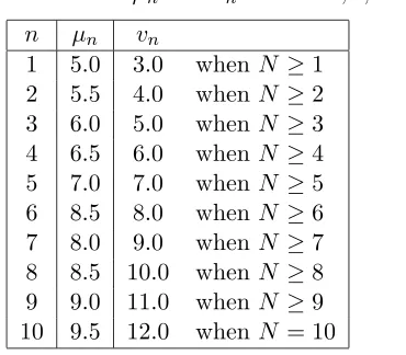
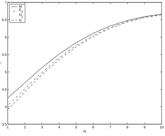
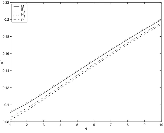
We consider three instances of G/M(n)/1/K queueing system with K = 10 and mean interarrival time 1/8. The arrival processes considered are Poisson, 3-stage Erlang and hyperexponential respectively. The values ofµnare given in Table 2.1 and the vacation

rate is 12. N is varied from 1 to 10 and the blocking probability PB, the average number

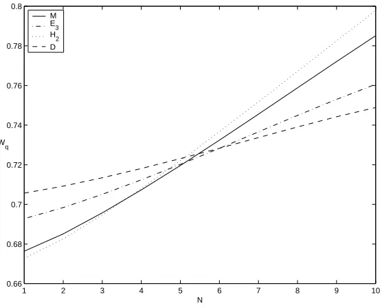
of customers in the system L and the waiting time in queue Wq are calculated for each instance. Each of these measures is plotted againstN for the different arrival distributions (See Figures 2.1, 2.2 and 2.3).

Table 2.1: Values of µnfor n= 1,2, . . . ,10

n µn

1 5.0 2 5.5 3 6.0 4 6.5 5 7.0 6 8.5 7 8.0 8 8.5 9 9.0 10 9.5

For Poisson arrival with mean interarrival time 1/8, the interarrival time distribu-tion and the Laplace-Stieltjes transform are given as follows

a(x) = 8e−8x A(x) = 1−e−8x

e

A(s) = 8 8 +s

For 3-stage Erlang arrival process (E3) with mean interarrival time 1/8, the inter-arrival time distribution and the Laplace-Stieltjes transform are given as follows

a(x) = 24e−24x(242!x)2

A(x) = 1− 2

X

r=0

e−24x(24x)

(33)

e

A(s) =

Ã

24 24 +s

!₃

For hyperexponential arrival process with q1 = 0.4, q2 = 0.6 and λ1 = 16,λ2 = 6 (mean interarrival time = 1/8), the interarrival time distribution and the Laplace-Stieltjes transform are given as follows

a(x) = 0.4∗16e−16x+ 0.6∗6e−6x A(x) = 0.4(1−e−16x) + 0.6(1−e−6x)

e

A(s) = 0.4

Ã

16 16 +s

!

+ 0.6

Ã

6 6 +s

!

For deterministic arrival with interarrival time = 1/8, the interarrival time distri-bution and the Laplace-Stieltjes transform are given as follows

e

A(s) = e−s/8

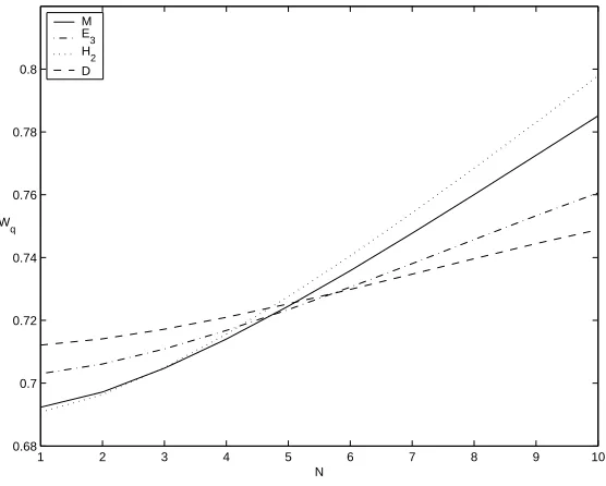
In figure 2.1, we see thatLis higher for the interarrival time distribution with the lower variance. It is also seen thatLincreases with increasing N. Also from figure 2.2,Wq

is lower for the interarrival time distribution with the higher variance when N is 1. AsN

increases Wq increases, with the increase inWq more for the interarrival time distribution with the higher variance. Once N crosses 6, Wq is found to be higher for the interarrival

time distribution with the higher variance. And from figure 2.3 the blocking probability

PBis lower for the interarrival time distribution with the lower variance. AlsoPB increases

with increasing N.

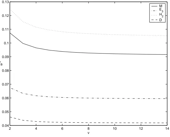
Now, we try to see how the vacation rate v influences the system performance measures. We consider a G/M(n)/1/K queueing system with K = 10, N = 3 and mean inter arrival time 1/8. vis varied from 2 to 14 and the blocking probabilityPB, the average

number of customers in the systemL and the waiting time in queue Wq are calculated for

each instance. Each of these measures is plotted againstv for the different arrival distribu-tions (See Figures 2.4, 2.5 and 2.6).

In figure 2.4, we see thatLis higher for the interarrival time distribution with the lower variance. It is also seen that Ldecreases with increasing v. Also from figure 2.5,Wq

(34)

with the higher variance. Oncevcrosses 8,Wqis found to be lower for the interarrival time

distribution with the higher variance. And from figure 2.6 the blocking probability PB is

lower for the interarrival time distribution with the lower variance. AlsoPB decreases with

(35)

1 2 3 4 5 6 7 8 9 10 5.7

5.8 5.9 6 6.1 6.2 6.3 6.4 6.5 6.6 6.7

N L

M E₃ H

2

D

Figure 2.1: Effect ofN on Lfor interarrival time distributions M,E3,H2 and D

1 2 3 4 5 6 7 8 9 10

0.66 0.68 0.7 0.72 0.74 0.76 0.78 0.8

N W

q

M E

3

H

2

D

(36)

1 2 3 4 5 6 7 8 9 10 0.04

0.06 0.08 0.1 0.12

N P

B

M E

3

H

2

D

Figure 2.3: Effect ofN onPB for interarrival time distributions M,E3,H2 and D

2 4 6 8 10 12 14

5.8 5.9 6 6.1 6.2 6.3 6.4 6.5 6.6

v L

M E

3

H₂ D

(37)

2 4 6 8 10 12 14 0.69

0.7 0.71 0.72 0.73 0.74 0.75 0.76

v W_q

M E₃ H

2

D

Figure 2.5: Effect ofv on Wq for interarrival time distributionsM,E3,H2,Dand N=3

2 4 6 8 10 12 14

0.04 0.05 0.06 0.07 0.08 0.09 0.1 0.11 0.12 0.13

v P

B

M E

3

H

2

D

(38)

Chapter 3

G/M(n)/1/K queue with

state-dependent vacations

3.1 Model Description

In this system, we assume that the inter arrival times are independently and iden-tically distributed (i.i.d.) with general distribution A(x)(x ≥ 0) and probability density function (p.d.f.) a(x)(x ≥ 0) and mean interarrival time E(A). Arriving units at the server form a single waiting line and are served in the order of their arrivals i.e., the ser-vice discipline is FIFO. The serser-vice times for successive customers are independently and exponentially distributed with parameter µn where n is the number of customers in the system. As soon as the system becomes empty the server is turned off and takes a vacation of random length with Pr[V ≤t] = 1−e−vnt_{. The server takes repeated vacations}_V _until

there are at leastN(N ≥1) customers to be served on return from a vacation. Once service is started, the server will continue service until the queue is exhausted.

(39)

the expected waiting time, average queue length, etc. Next we develop a recursive algo-rithm for numerically computing the stationary queue length distribution in theN policy

G/M(n)/1/K queues with multiple state-dependent exponential vacations. The complex-ity of the algorithm is O(n3). Then we illustrate the algorithm by presenting a few simple examples.

Notations and probabilities

The two-dimensional state-space of the system is defined as

{(i,n) : (i= 0 and n= 0,1, . . . , K) or (i= 1 and n= 1,2, . . . , K)} The following notations are used in this chapter

N – threshold level

K – system capacity (N ≤K)

A(x) – c.d.f. of interarrival time A a(x) – p.d.f. of interarrival timeA

e

A(s) – Laplace-Stieltjes transform of interarrival timeA

e

A(l)(s) – lth order derivative ofAe(s) with respect tos

P1,n(t) – probability ofncustomers in the system at time twhen the server is working, wheren= 1,2, . . . , K

e

Pi,n(s) – Laplace-Stieltjes transform ofPi,n(x) wherei= 0,1

e

P_i,n(l)(s) – lth order derivative ofPei,n(s) with respect tos

E(A) – mean interarrival time

vn – vacation rate of the system in state (0, n), where n= 0,1, . . . , K

µn – service rate of the system in state (1, n), wheren= 1,2, . . . , K

P₀−_,n – probability ofncustomers in the system immediately prior to an arrival when the server is idle

P₁−_,n – probability ofncustomers in the system immediately prior to an arrival when the server is busy

PB – probability an arriving customer is blocked because the system is full

L – average number of customers in the system

(40)

Wq – average waiting time in the queue

λ0 – effective arrival rate into the system

3.2 Formulation

We first establish the mathematical equations to govern the system by employing the remaining interarrival time as the supplementary variable. Next, we develop a recursive method to derive the steady-state probability distributions of the number of customers in the system.

The state of the system at timetis given by [Q(t), U(t)], where

Q(t) – number of customers in the system at timet

U(t) – remaining interarrival time for the customers who is arriving

Let us define

P0,n(x, t)dx = Prob{Q(t) =n, x < U(t)≤x+dx, server is on vacations}, x≥0, n= 0,1, . . . , K

P1,n(x, t)dx = Prob{Q(t) =n, x < U(t)≤x+dx, server is busy},

x≥0, n= 1,2, . . . , K

Relating the state of the system at timetand t+dt, we set up the following partial differ-ential equations

−∂P0,0(x, t)

∂x +

∂P0,0(x, t)

∂t = µ1P1,1(x, t) (3.1)

−∂P0,n(x, t)

∂x +

∂P0,n(x, t)

∂t = a(x)P0,n−1(0, t), 1≤n≤N −1 (3.2)

−∂P0,n(x, t)

∂x +

∂P0,n(x, t)

∂t = a(x)P0,n−1(0, t)−vnP0,n(x, t), N ≤n≤K−1 (3.3)

−∂P0,K(x, t)

∂x +

∂P0,K(x, t)

∂t = a(x)[P0,K−1(0, t) +P0,K(0, t)]−vKP0,K(x, t) (3.4)

−∂P1,1(x, t)

∂x +

∂P1,1(x, t)

(41)

−∂P1,n(x, t)

∂x +

∂P1,n(x, t)

∂t = a(x)P1,n−1(0, t) +µn+1P1,n+1(x, t)−µnP1,n(x, t),

2≤n≤N−1 (3.6)

−∂P1,n(x, t)

∂x +

∂P1,n(x, t)

∂t = vnP0,n(x, t) +a(x)P1,n−1(0, t) +µn+1P1,n+1(x, t)

−µnP1,n(x, t), N ≤n≤K−1 (3.7)

−∂P1,K(x, t)

∂x +

∂P1,K(x, t)

∂t = vKP0,K(x, t) +a(x)[P1,K−1(0, t) +P1,K(0, t)]

−µKP1,K(x, t) (3.8)

In steady state, we define,

P0,n = lim

t→∞P0,n(t), n= 0,1, . . . , N, . . . , K

P0,n(x) = _tlim_→∞P0,n(x, t), n= 0,1, . . . , N, . . . , K

P1,n = _tlim_→∞P1,n(t), n= 1,2, . . . , N, . . . , K

P1,n(x) = lim

t→∞P1,n(x, t), n= 1,2, . . . , N, . . . , K

From (3.1)– (3.8), steady-state equations are obtained as follows

−dP0,0(x)

dx = µ1P1,1(x) (3.9)

−dP0,n(x)

dx = a(x)P0,n−1(0), 1≤n≤N−1 (3.10)

−dP0,n(x)

dx = a(x)P0,n−1(0)−vnP0,n(x), N ≤n≤K−1 (3.11)

−dP0,K(x)

dx = a(x)[P0,K−1(0) +P0,K(0)]−vKP0,K(x) (3.12)

−dP1,1(x)

dx = µ2P1,2(x)−µ1P1,1(x) (3.13)

−dP1,n(x)

dx = a(x)P1,n−1(0) +µn+1P1,n+1(x)−µnP1,n(x), 2≤n≤N −1 (3.14)

−dP1,n(x)

dx = vnP0,n(x) +a(x)P1,n−1(0) +µn+1P1,n+1(x)−µnP1,n(x),

N ≤n≤K−1 (3.15)

−dP1,K(x)

(42)

We define the following Laplace-Stieltjes transforms,

e

A(s) =

Z _∞

0 e

−sx_a₍_x₎_dx

e

Pi,n(s) =

Z _∞

0 e

−sx_P

i,n(x)dx, i= 0,1

Pi,n = Pei,n(0) =

Z _∞

0 Pi,n(x)dx, i= 0,1

Z _∞

0 e

−sx ∂

∂xPi,n(x)dx = sPei,n(s)−Pi,n(0)

Taking Laplace-Stieltjes transforms on both sides of (3.9)– (3.16), we obtain the following

−sPe0,0(s) = µ1Pe1,1(s)−P0,0(0) (3.17)

−sPe0,n(s) = Ae(s)P0,n−1(0)−P0,n(0), 1≤n≤N−1 (3.18)

(vn−s)Pe0,n(s) = Ae(s)P0,n−1(0)−P0,n(0), N ≤n≤K−1 (3.19)

(vK−s)Pe0,K(s) = Ae(s)[P0,K−1(0) +P0,K(0)]−P0,K(0) (3.20) (µ1−s)Pe1,1(s) = µ2Pe1,2(s)−P1,1(0) (3.21) (µn−s)Pe1,n(s) = µn+1Pe1,n+1(s) +Ae(s)P1,n−1(0)−P1,n(0), 1≤n≤N −1(3.22) (µn−s)Pe1,n(s) = vnPe0,n(s) +µn+1Pe1,n+1(s) +Ae(s)P1,n−1(0)−P1,n(0),

N ≤n≤K−1 (3.23)

(µK−s)Pe1,K(s) = vKPe0,K(s) +Ae(s)[P1,K−1(0) +P1,K(0)]−P1,K(0) (3.24) Substituting s=0 in (3.17), we get

P0,0(0) = µ1Pe1,1(0) = µ1P1,1

Substituting s=0 in (3.18), we get

(43)

Differentiating (3.18) w.r.ts,

e

P0,n(0) = −Ae(1)(0)P0,n−1(0), 1≤n≤N−1

⇒P0,n = E(A)P0,n−1(0), 1≤n≤N−1 (3.26) Substituting s=vn in (3.19) and (3.20),

P0,n(0) = Ae(vn)P0,n−1(0), N ≤n≤K−1

P0,N(0) = Ae(vN)P0,N−1(0) = Ae(vN)P0,0(0)

⇒P0,n(0) = [

n

Y

i=N

e

A(vi)]P0,0(0), N ≤n≤K−1 (3.27) (1−Ae(vK))P0,K(0) = [

K

Y

i=N

e

A(vi)]P0,0(0)

P0,K(0) = [

Q_K

i=NAe(vi)]P0,0(0) 1−Ae(vK)

(3.28)

Substituting s=0 (3.19) and (3.20),

vnPe0,n(0) = Ae(0)P0,n−1(0)−P0,n(0), N ≤n≤K−1

⇒Pe0,n(0) = P0,n−1(0)−P0,n(0)

vn , N ≤n≤K−1

⇒P0,n = 1

vn[1−

e

A(vn)][ n_Y−1

i=N

e

A(vi)]P0,0(0), N ≤n≤K−1 (3.29)

vKPe0,K(0) = P0,K−1(0)

⇒P0,K = [

Q_K₋₁

i=N Ae(vi)]P0,0(0)

vK (3.30)

Adding equations (3.17) to (3.24) and simplifying we obtain,

K

X

n=0

e

P0,n(s) + K

X

n=1

e

P1,n(s) = 1−

e

A(s)

s

h_XK

n=0

P0,n(0) + K

X

n=1

P1,n(0)

Single and Multiple Server Queues with Vacations: Analysis and Algorithms

Contents

List of Figures

List of Tables

Chapter 1

Introduction

1.1

Background

1.2

Problem Definition

1.3

Literature Review

1.4

Organization of Thesis

Chapter 2

G/M(n)/1/K queue with

exponential vacations

2.1

Model Description

2.2

Formulation

2.3

Analysis

2.4

Algorithm

Chapter 3

G/M(n)/1/K queue with

state-dependent vacations

3.1

Model Description

3.2

Formulation