Export-Led Growth Hypothesis: An Analysis Of India’s Post Liberalization Experience

(1)

1489

Export-Led Growth Hypothesis: An Analysis Of

India’s Post Liberalization Experience

Ho Man Giang, Ibrahim Nurudeen

Abstract : This study empirically examines the relationship among GDP, import and export by investigating the validity of the export-led growth hypothesis in India. A quarterly data that spanned from 1996.Q2 to 2019Q2 has been employed for the analysis of the study. The stochastic properties of the series checked through Philips and Perron (1988), finds all the three series to be stationary at first difference, and this has further been examined through Perron (1997), which confirms the presence of a unit-root with structural breaks in the crash, growth, and crash-growth models at different dates. A Johansen test of co-integration reveals the presence of two co-integrating relations, and the short-run dynamics coefficient reveals that 50 percent of the disequilibrium in the system is being corrected every quarter. The study further finds the evidence of a long-run causality between export and GDP, although not in the short run. Thus, the study wrapped up by lending support for the validity of the export-led growth hypothesis to the Indian economy. Keywords: GDP, Export, Import, stationary, Johansen

————————————————————

1.0 INTRODUCTION

The role of export in improving the growth of a nation could not be overemphasized. It has attracted the attention of experts especially in the area of development economics. Thus, it remains the goal of every economy to find ways of growing the economy sustainably. One such areas identified by the expert is to encourage export which in turn leads to growth and development of the economy, hence reduce the current account deficit and boost the value of the local currency. When exports are encouraged, it allows the economy to compete with the rest of the world, and hence motivates innovations and inventions through the adoption of new technology. Moreover, the local entrepreneurs will be forced to imbibe the imported technology so easily and rapidly, this in essence, increases productivity thereby positively affecting the overall growth of the nation. There are several efforts to find the relationship between export and economic growth of different economies. See, for example, Beckerman 1965, Balassa 1978, 1985, Romer 1986, and Gilles and Williams 2000, etc. Some studies had concluded in support of Export-led Growth Hypothesis (from now ELGH), which implies the existence of a long-run relationship between export and GDP, and thus, export is found to have caused GDP, for example, see the works of Agrawal (2014), Ahmad, Kostelic, and Ahmad (2016), Maneschiold (2008), Assaf and Al-Abdulrazaq (2015), Balassa (1978), and Tyler (1981), etc. Contrariwise, some studies concluded without finding the evidence to support the existence of ELGH in some countries, this finding could be found in the works of Tahir, Khan, Israr, and Abdul Qahar (2015). Similarly, in the case of India, a lot of ink has been spilt in search of the evidence for or against ELGH. Studies that had found the evidence to be in support of ELGH in India include a research conducted by Agrawal (2015), who found the validity of ELGH for the Indian post-liberalization period, however, the evidence was not the same for the pre-liberalization period, this might not be unconnected with the opening of the economy in the post-liberalization period, where the main policy at the period was to shift the economy from the import substitution to export promotion. Other efforts to find the validity of the hypothesis for the Indian economy include the works of Sahni and Atri (2012), Kumari and Malhotra (2014), Guntukula (2018), and Kumar (2012), etc. Whereas all the above studies use the linear

modelling approach to study the relation between the two series, we have in addition to that, incorporated the non-linear modelling approach for the robustness of the result. India opens its economy in 1991, where growth was targeted through the expansion of export. As a part of liberalization, India became a member of the WTO in 1992; this also was expected to correct the increasing budget deficit and foreign debt and to address the growing difference between income and expenditure of the country, which created a serious current account crisis. Part of the liberalization process by the government of Narasinha Rao was the reduction of a large number of import and export items, which paved the way for the private sector to also come forward and participate in the reviving and revamping of the economy. Some of the export promotion measures taken at the time include among others, creation of Export Promotion Capital Scheme, Export Promotion Capital Scheme for the service sector, expansion of Export Processing Zones(EPZ), duty-free import for export under advance licensing scheme, establishment of Special Economic Zones, and establishment of window at the Ministry of Commerce to deal with issues faced by the exporters. Moreover, in addition to the above efforts, the inflow of foreign capital has also been liberalized in order to encourage Foreign Direct Investment.

1.1 Trend of Trade in India

(2)

1490

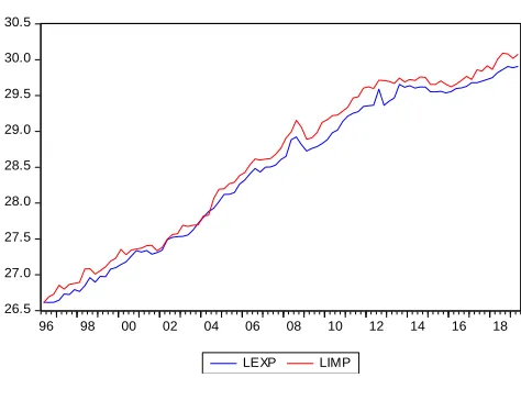
that both series are increasing at the same time, and it has been a deficit for the whole quarters, except 2003Q4, and 2004Q2. There was a sharp break in both series in 2008Q3, this was the period when the financial crisis set in, in the US, though the Indian economy did not experience too much hit of the crisis in 2008, however, some of the sectors were affected. There was a slowdown in the economy from 2013Q2 which persisted till today, this might not be unconnected with the withdrawal of institutional investors that resulted in the repatriation of a large amount of capital abroad, and also this resulted in the decline of both export and import of the country

Figure 1: LEXP and LIMP

26.5 27.0 27.5 28.0 28.5 29.0 29.5 30.0 30.5

96 98 00 02 04 06 08 10 12 14 16 18

LEXP LIMP

2.0 LITERATURE REVIEW

In this section, we review some of the studies related to this research. Different studies have been undertaken in this area related to different economies, while some studies have findings in support of the ELGH; however, some findings couldn’t find the evidence.

Maneschiold (2008), examines the ELGH for Argentina, Brazil and Mexico using a time series approach. Johansen co-integration procedure and Granger causality were applied to determine the long-run relationship and the direction of causality between the variables for the three countries. The findings of the study reveal that there is a co-integrating relation found for Argentina and Mexico, which implies the existence of a long-run relationship between export and GDP, however, no such relationship is found for Brazil. Similarly, the causality test conducted reveals the existence of bi-directional causality between export and GDP for both Argentina and Mexico, however, in the case of Brazil, the Granger causality test, reveals the existence of unidirectional causality which runs from export to GDP. Hence, the overall findings lend support for export-oriented growth in order to enhance the growth and development of those nations. In the same vein, Al-Assaf and Abdul-Razaq (2015), examine the validity of ELGH for Jordan using the same procedure with the above study. However, instead of the Johansen procedure of co-integration as used by Maneschiold (2008), ARDL procedure was used. The short-run and long-short-run analysis reveal that there is a long-short-run relationship between export and GDP lending support for ELGH; hence export is a strong stimulant to economic growth and development of Jordan. Ahmad, Kostelic, and Ahmad (2016) also used the same ARDL procedure as in

the case of Al-Assaf and Abdul-Razaq (2015) for Pakistan, the findings of their study reveal that 1 percent increase in export will raise GDP by 1.11 percent in the long run and a 1 percent increase in export will raise GDP with1.34 percent in the short run, hence lending a support for the validity of ELGH in Pakistan. Contrariwise, Tahir, Khan, Israr and Abdul Qadir (2015), could not find the evidence of a long-run relationship between export and GDP, after adopting the same econometric procedure with the above studies. Moreover, the granger causality test supports to the earlier finding of the Johansen procedure of co-integration, thus, no long-run relationship and no causality from both directions, hence, failed to find support for ELGH for the Sri Lankan economy in the post-liberalization period. This was the finding of Shiraz and Abdul Manap (2005), they have considered five Asian countries that include, Pakistan, Sri Lanka, India, Bangladesh and Nepal. A co-integration analysis was conducted in search of the evidence for or against the hypothesis, and a causality test has also been conducted through Toda Yamamoto (1996). The evidence shows the validity of ELGH for all the countries except Sri Lanka, which implies that Tahir, Khan, Israr and Abdul Qadir (2015), the finding is backed by Shiraz and Abdul Manap (2005), findings. Different studies have been put in place, to investigate the applicability of ELGH to the Indian economy. Sahni and Atri (2012), applied the ordinary least square procedure, to estimate the relationship between export, Manufactured import, GNP, and investment. The study, finds export to be an important variable that determines the growth of India, hence lends support for the ELGH in India. Kumara and Malhotra (2014), couldn’t establish the evidence validity of the ELGH in their study, although they have used Johansen test of co-integration, which is multivariate and dynamic in the specification, which are the major differences with the study of Sahni and Atri (2012). Despite being a higher model for its inclusion of historical components into the specification, the finding of Kumari and Malhotra (2014), could be misleading, because the analysis covers a period of 1980 to 2014, which means, that the period when India opens its economy(Liberalization period) has not been taken into consideration, hence, to better investigate the validity of the hypothesis to the Indian economy, a pre and post-liberalization periods needs to be studied separately, or else one of the non-linear models should be used to check the validity of such hypothesis. In the vane vein, Agrawal (2014), investigates the validity of the hypothesis, by considering pre- and post-liberalization periods. The post-liberalization period is found to be consistent with the hypothesis, this is obvious because post-liberalization is the period when India opens its economy to the rest of the world. Thus, the pre liberalization period failed to be consistent with the hypothesis. This is more realistic than the previous study because Agrawal (2015) has analyzed pre- and post-liberalization periods separately.

3.0 METHODOLOGY

3.1. Data and Variables

(3)

1491

and the three series are sourced from the Reserve Bank of St. Louis.

3.2. Econometric Procedure

The analysis was carried out first by checking the stochastic properties of the series using Philips and Perron(1988) test of unit-root, this was followed by a unit-root test with break developed by Perron(1997). To understand the application of both Philips and Perron(1988), and Perron(1997), first consider the following equation which represents specification for Philips and Perron(1988):

et

pY

Y

_t





_t



_t







_₁



(1)

Where the null alternative of unit-root is to be accepted if

1 

p

, however, if

p



1

then the alternative is to be accepted.Perron(1997), is an extension of Perrron(1989), the model for the unit-root test in the presence of one exogenous break. The application of the model is presented below:



  







k i t t t b

t

DUT

t

D

T

y

Dy

et

y

1 1 1

)

(









(2)

Where

DU

_t= 1 if

t

>

T

_b, 0 otherwise

and,

D

(

T

_b

)

_t



1

if

t



T

_b



1

, 0 otherwise

Above is known as a crash model in Perron (1989) specification, it tests the null of unit-root in the presence of break at an unknown date against the alternative of stationarity in the presence of break at an unknown date. We are therefore to accept null if





1

, and we are to accept alternative is it is less than one, and therefore the series is explosive in case it is greater than 1. Below is the specification of the growth model (B Model).

et

Dy

y

T

D

DT

t

DU

y

k i t t t b t

t









   1 1 1

)

(















(3) Where

DT

b



1

if

t



(

T

b

)

tand 0 otherwise

Here, a null of unit-root in the presence of break-in both intercept and trend is tested against the alternative of stationarity in the presence of break-in both intercept and trend. Thus, the series is stationary if





1 ,

otherwise, the

series has a unit root, if





1

. The third model which is model C or the crash-growth model assumes break to only affect the trend. To understand the model, consider the specification below:

t t

t

DT

y













* (4)

Where

DT

*t=1 if

(

t



T

_b

)(

t



T

_b

)

and 0 otherwise.



  





k i t t

t

y

D

y

et

y

1 _ 1 1 _ _





(5)

Where models (4) and (5) are the regression line of the breaking series, and the auxiliary regression line respectively. The Johansen Procedure of testing co-integrating relations was the procedure employed to check the evidence or otherwise of a long-run relationship among

our variables. However, the specification of the Johansen procedure is skipped due to space limitation.

4.0 RESULT

PRESENTATION

AND

DISCUSSION

This section presents the result and discussion of the analysis. In the tables below, we present the result of each test conducted separately.

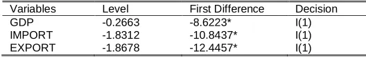
Table 1: Philips and Perron Test of Unit-Root

Variables Level First Difference Decision

GDP -0.2663 -8.6223* I(1)

IMPORT -1.8312 -10.8437* I(1)

EXPORT -1.8678 -12.4457* I(1)

Philips and Perron’s critical values, 4.243644, 3.544284, and -3.204699 for 1% level, 5% level, and 10% level respectively. *, **, and *** Denotes rejection of null hypothesis at 1%, 5%, and 10% levels of significance respectively.

Table 1, presents the unit root analysis, conducted through Philips and Peron. The idea behind the unit-root testing is to determine the stochastic properties of each series, this informs us of the stability situation of the series. The result in table 1 shows that all series are not stationary at level, because when we compare the critical values with the calculated values, it appears that, the critical values are greater at 1, 5 and 10 percent, therefore, this implies the acceptance of null hypothesis of unit-root against the alternative of no unit-root. Similarly, after taking the first difference of all the series, they all became stationary at 1 percent, and this implies that the alternative hypothesis is accepted and null hereby rejected. Thus, we conclude by saying all our series are stationary at first difference. i.e. I (1). In order to have a robust finding of the conclusion drawn from the above unit-root test, we subject all the series to a Perron(1997) unit-root test with a structural break, below is the result and discussion of the output.

Table 2: Perron (1997) Test of Unit-Root with Break

Variables Model A Break Date Lags Decision

GDP -1.8473 2015Q1 4 Accept Null

IMPORT -2.9756 2009Q3 4 Accept Null EXPORT -3.1605 2010Q3 4 Accept Null

Model B

IMPORT -3.3860 2009Q3 4 Accept Null EXPORT -3.6415 2010Q1 4 Accept Null

Model C

IMPORT -3.0966 2004Q3 4 Accept Null EXPORT -3.7049 2005Q2 4 Accept Null Model A Null: Has unit-root with a structural break in the intercept. Model B Null: has uni-root with the structural break in both intercept and trend, Model C: Null: Has uni-root with the structural break in trend.

(4)

1492

a null of unit-root with structural break in the intercept is tested against the alternative of no unit-root with structural break in the intercept while Model B(Growth Model) tests the null of unit-root with structural break in both intercept and trend, and lastly, Model C(Crash and Growth) where null of unit-root with structural break in trend is tested. The idea of first Zivot and Andrew (19920), and later Perron (1997), was to come up with a test where an important break date is determined by the data endogenously. Thus, the three series couldn’t reject the null of unit-root with a structural break in all the three models, this further confirms the evidence of derived in the Philips and Perron(1988) test without break. The important event(break) happens in different dates of the series, for example, GDP series has broken in 2015Q1, 2009Q2, and 2013Q2 for model A, B, and C respectively. In 2015, there was oil glut which affects the confidence of the investors especially in the crude oil sector, this is likely the cause of the break in the GDP this year. The year 2009 was the year when the world experienced one of the worst world’s recession in 2008, though Indian economy was not hit much in that year fear in the heart of investors, might be the major the reason why the Indian output experienced a break. In 2013, there was a continuous upsurge in the value of the dollar against the Indian rupee which was triggered by the large capital outflows, and hence the Indian rupee was depreciated by almost 13.7 percent. The year 200, Was the year when the Indian import experienced a break in both A and B models, and this might not be unconnected with the financial crisis of 2008. Indian export also experienced a major break in 2010 in both A and B models, this is also might not b unconnected with the decline of India’s gross capital formation from 39.8 percent in 2010 to 28.6 percent in 2017.

Table 3 Pantula Method for Choosing Co-Integrating

Equations

Number of Co-integrating equations Trace statistic Max. Eig.

Val No Intercept or trend in CE or VAR 1 1 Intercept (no trend) in CE. No

intercept in VAR 1 1

Intercept (no Trend) in CE in test

VAR 2 2

Intercept and Trend in CE no

Intercept and Trend in CE

Table 3, presents a co-integration analysis of conducted through Johansen test of co-integration. a Pantula method of choosing co-integration was employed which suggests all the five assumptions to be adopted in searching for the co-integration and hence adopt any of the assumptions which have the highest co-integrating relations. In the analysis conducted, intercept (no Trend) in CE in test VAR has the highest co-integrating relations for both Maximum Eigenvalue and Trace statistic.

Table 4: Long run equation

Euqation/Variables GDP EXPORT IMPORT GDP 1.00000 13.4854(6.809) -14.090(5.791) Standard error in parenthesis.

A Johansen test helps us in determining the long-run relationship between variables in a case where individual variables have integration, and thus long-run integration is established through Johansen. Since we found two co-integrating relations among our variables, we have extracted the long-run model from the Johansen test. The long-run model is reported in table 4, and when we normalize on GDP, the result shows that in the long run GDP will have a positive relationship with export, which implies that increase in India’s output has a potential to increase the export and vice versa. This outcome conforms with the theoretical expectation. Hence India’s post-liberalization time series data support the evidence of export-led growth hypothesis. However, the direction of long-run causality will examine in table 7, of this analysis. Moreover, import appears to have a long-run negative relationship with GDP, this means that too much of import to India is injurious to the economy, and hence, monetary and fiscal policies should be put in place to keep the import within the green line.

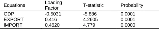
Table 5: Coefficients of the Speed of adjustment

Equations Loading

Factor T-statistic Probability

GDP -0.5031 -5.886 0.0001

EXPORT 0.416 4.2605 0.0001

IMPORT 0.4620 4.779 0.0000

(5)

1493

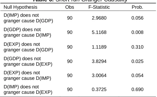
Table 6: Short-run Granger Causality

Null Hypothesis Obs F-Statistic Prob. D(IMP) does not

granger cause D(GDP) 90 2.9680 0.056 D(GDP) does not

granger cause D(IMP) 90 5.1168 0.008 D(EXP) does not

granger cause D(GDP) 90 1.1189 0.310 D(GDP) does not

granger cause D(EXP) 90 3.8294 0.025 D(EXP) does not

granger cause D(IMP) 90 3.0064 0.054 D(IMP) does not

granger cause D(EXP) 90 0.3725 0.690

Table 6, presents the result of the short-run causality, which was conducted through granger causality. Granger causality is applied in two situations, when all variables are level stationery or when all the variables stationary at first difference. In the case of this study, the variables in the analysis are stationary at first difference; hence differenced granger causality is applied. This implies that the resultant of the test is only applicable in the short run. Hence, in the short run export does not granger cause GDP, this means that however, there is a short-run bi-directional causality that runs from GDP to export, which implies that, in the short-run GDP cause export and not vice versa. Since we couldn’t establish a causal effect of export to GDP in the short run, we now investigate if the export is a potential variable for causing GDP in the long run, this done with the help of Wald test.

Table 7; Long-run Causality Test

Equations/Variables GDP Export Import

GDP 1 4.6711(0.0001) -1.2697(0.20)

IMPORT - - -

EXPORT - - -

Probability values in parenthesis

The result in table 7, shows the long-run causality test among GDP, export and import. There is a strong evidence of causal relationship which runs from export to GDP in the long run, the T statistic is reported in table 7 above which shows that export is significant at 1 percent level of significance in explaining GDP in the long run, this has conformed with the theoretical expectation that export causes GDP in the long run, however, such is not the case for import, as its probability of causing GDP, in the long run, is 20 percent. This further confirms the outcome of the long-run model which extracted through the Johansen test of co-integration.

5.0 CONCLUSION

The study examines the relationships among GDP, import and export of India by investigating the validity of the export-led growth hypothesis in the post-liberalization period. The result of the study reveals that the variables in the study are integrated of order one, which has been confirmed by the unit-root test with a break. A long-run relationship among the series that was conducted through Johansen established the evidence of the long run

co-integrating relations. The short-run dynamics of the study also revealed that 50 percent of the disequilibrium in the system gets corrected in every quarter. The long-run causality between GDP and export reveal that export cause GDP in the long-run. Although in the short- run, the study reveals that, export could not cause GDP, however, GDP is found to be an important variable in causing GDP in the short-run. Thus, the study lends support and concluded in favour of the export-led growth hypothesis. It is therefore, recommended that since export is a potential series in causing movement in India’s output then policies should be placed not only stimulate the growth but also sustain it in order to ensure growth and development in the nation, this policy could be curtailing of the stringent procedures in obtaining export and import license, and also ensure a compliance with the quality standard of the receiving country.

6 REFERENCE

[1]. Aggarwal P., (2014), The role of Export in India’s Economic Growth. IEG Working Paper No. 345

[2]. Al-Assaf G., and Abdulrazaq B., (2015), The validity of export-led growth hypothesis for Jordan. A bound testing approaches. International Journal of Economics and Financial Issues Vol. 5, No. 1, 2015, pp.199-211ISSN: 2146-4138.www.econjournals.com [3]. Ahmad N., Kostelic N, and Ahmad K., (2016), Is

export Led-Growh Hypothesis valid in Pakistan. If so, how relevant is export to Europe? European Union future perspective: Innovation, Enterpreneurship, and Economic Policy

[4]. [Balassa, B. (1978). Export and economic growth: further evidence. Journal of development economics 5, no 2:181-89. [5]. Guntukula R., (2018), Export, Import, and

Economic Growth in India: Evicdence from Co-integrationa and Causality Analysis,Theoretical and Applied Economics Volume XXV (2018), No. 2(615), Summer, pp. 221-230

[6]. Granger C. W. J. (1969), Investigating Causal Relationship by Econometric Models and Cross Spectral Analysis. Econometrica 37. No.3. 424-38

[7]. Johansen, S. (1988). Statistical analysis of cointegration vectors. Journal of Economic Dynamics and Control, Vol. 12: 231-254. [8]. Kumar G., (2015), Export Led-Growth

Hypothesis: Further Econometrics Evidence from India. Economic Affairs. DOI: 10.5958/0976-4666.2015.00029.7

[9]. Kumari D, and Malhotra N., (2014), Export Led-Growth in India: Co-integration and Causality Analysis. Journal of Economics and Development Studies Vo: 2 No.2, PP 297-310. ISSN: 2334-2382 (Print), 2334-2390 (Online [10]. Maneschiold P. O., (2008), A Note on the

export-led growth hypothesis: A time series approach

(6)

1494

[12].Perron, P., 1997. Further Evidence from Breaking Trend Functions in Macroeconomic Variables. Journalof Econometrics 80, 355–385. [13].Perron, P., 1989. The Great Crash, the Oil Price Shock and the Unit Root Hypothesis. Econometrica 57,

[14].1361–1401.

[15].Shirazi N., S.,and Abdul Manap T. A., (2005), Export Led Growth Hypothesi: Further econometric Evidence from South Asia. The Developing Economies

[16].Sahni P., and Atri V. N., (2012), Export Led-Growth Hypothesis in India: AN Empirical Investigation. Vol: 2, Issue 7. ISSN:2249-1058 [17].Tahir M, Khan M., Israr M., and Abdul

Qahar(2015), An analysis of export Led-Growth Hypothesis: Co-integration and Causality Evidence from Sri lanka. Advances in Economics and Business3(2):62-69 DOI: 10.13189/aeb.2015.030205

[18].Tyler W.G. (1981) Growth and export expansion in developing countries: some empirical evidence, Journal of Development Economics, 9, 121-30

AUTHORS:

Author 1 Ho Man Giang

PhD scholar, Economics Dept, Madras University, Chennai, India

Mobile: +84 935079094

Email: [email protected]

Author 2 Ibrahim Nurudeen

Department of Economics, Shehu Shagari College of Education, Sokoto, Nigeria Mobile: +234 8067677676