A General Monte Carlo Method for Mapping Multiple Quantitative Trait Loci

(1)

A General Monte Carlo Method for Mapping Multiple Quantitative Trait Loci

Ritsert

C. Jansen

Centre for Plant Breeding and Reproduction Research, 6700 AA Wageningen, The Netherlands

Manuscript received May 1 , 1995

Accepted for publication October 4, 1995

ABSTRACT

In this paper we address the mapping of multiple quantitative trait loci (QTLs) in line crosses for which the genetic data are highly incomplete. Such complicated situations occur, for instance, when

dominant markers are used or when unequally informative markers are used in experiments with outbred populations. We describe a general and flexible Monte Carlo expectation-maximization (Monte Carlo

EM) algorithm for fitting multiple-QTL models to such data. Implementation of this algorithm is straightforward in standard statistical software, but computation may take much time. The method may be generalized to cope with more complex models for animal and human pedigrees. A practical example is presented, where a three-QTL model is adopted in an outbreeding situation with dominant markers.

The example is concerned with the linkage between randomly amplified polymorphic DNA ( W D ) markers and QTLs for partial resistance to Fusarium oxysporum in lily.

M

ANY traits of interest to plant, animal and human geneticists are controlled by genes of which the inheritance can hardly be assessed [quantitative trait loci ( QTLs)

3 .

The advent of molecular markers, however, heralded a new era for studying the genetics of such complex traits. In only a few years time the use of molecular markers has had a major impact on funda- mental plant and animal genetics and on human medi- cal genetics (TANKSLEY 1993; LANDER and SCHORK 1994). Moreover, many new and challenging problems have arisen at the interface of quantitative genetics and statistics. Currently, QTL mapping is a very active area of theoretical research.

QTL mapping can be viewed as a problem for which the data are incomplete: the observations of the genotypes at the QTLs are missing. Since genotypes at molecular marker loci are (generally) known, markers can be informative to reveal QTL genotypes. The interval mapping method (LANDER and BOTSTEIN 1989) has become the most widely used method for QTL analysis in line crosses. In a statistical sense the trait considered is regressed on a single putative QTL whereby the unknown QTL genotypes are deduced from flanking markers and phenotypic scores, by using an expectation-maximization (EM) algorithm. JANSEN ( 1992, 1994) and JANSEN and STAM (1994) developed a general and flexible EM algorithm for recovering information about a multiple-QTL genotype (“MQM mapping” ) , using all available marker and phenotypic data simultaneously. However, when many QTLs are in- cluded in a multiple-QTL model, computation may become unfeasible. We described an approximation of the genuine multiple-QTL model in which the presence

C’mresponding author: Ritsert C. Jansen, P.O. Box 16, 6700 A A , Wa-

geningen, The Netherlands. E-mail: [email protected]

of a single putative QTL is tested at different points along the chromosomes, while other putative QTLs are accommodated in the testing procedure by using information on markers associated with the QTLs ( a.e., ‘ se-

lected markers are used as “cofactors” in the model in a multiple regression context). We have shown that the efficiency and accuracy of QTL mapping can substan- tially be improved by applying MQM mapping instead of the widely used interval mapping method (JANSEN

1994). ZENC (1994) investigated a similar approach and came to similar conclusions.

In practice it is often the case that the marker genotypes are ambiguous or unknown. In addition to fortu- itously missing data, another type of missing marker data may occur in a natural way, namely when markers are dominant, or when unequally informative markers are used in experiments with outcrossing species. In the first case, the heterozygote cannot be distinguished from one of the homozygotes. In the second case, segregation and transmission cannot always be observed di- rectly. In line crosses some markers may segregate according to backcross rules ( a b X a a ) , so that the gametes from only one parent are informative, while other markers may segregate according to F2 rules ( a b

X a b ) , so that the gametes from both parents are informative. The interval under study for QTL activity may, for instance, be flanked by markers of the backcross type. Nearby markers of the F2 type may then provide additional information on the genotype of the putative QTL. Therefore it is important to use all available marker information simultaneously ( HALEY et al. 1994;

MALIEPAARD and VAN OOIJEN 1994; FULKER et al. 1995). Furthermore, QTLs and markers may segregate with three or four alleles per locus rather than with two alleles.

In the MQM mapping approach the missing QTL

(2)

and marker genotypes are deduced from all available information on phenotypes and marker genotypes simultaneously. For that purpose we consider the simulta- neous likelihood for the trait, all putative QTLs and all markers (and this is the main reason for abandoning the term "interval" mapping). Unfortunately, exact computation is virtually impossible with large populations when incomplete genetic data abound: the number of possible complete genotypes ( i . e . , compatible with available marker data) can be extremely large. In line crosses a solution to this problem can be to disre- gard unlikely genotypes (JANSEN and STAM 1994), which may work well in many practical cases (JANSEN et nl. 1995). However, for the situation we consider in this paper the set of possible genotypes is still too large. Similar computational problems may occur in the analysis of complex human pedigrees. To overcome the computational difficulties, Guo and THOMPSON (1992) in- troduced a Monte Carlo approach to the analysis of linkage between a single QTL and a single marker in human pedigrees. Here, we combine this approach and our original multiple-QTL approach. We focus on populations obtained from line crosses, because we are involved in such experiments, but the same ideas also apply to other types of population (for instance human pedigrees).

In the next two sections an "exact" EM algorithm and a Monte Carlo EM algorithm for multiple-QTL mapping are described. Finally a practical data set is analyzed.

EXACT EM

We consider a segregating population of N individuals obtained from line crosses (for instance backcross, F2 or doubled haploids). Let the random variables y i ,

h, and gi denote the phenotype, the incomplete genotype and a compatible complete genotype of individual i, respectively ( i = 1, 2

-

*

N)

.

Only y L and h, can be

observed. It should be noted that h, and g, may involve a large number of loci (marker loci and putative QTLs). We make the common assumption that the distribution f ( yi

I

g i ) of the phenotype given the complete genotype is a normal probability density function. Then, the distribution f ( yt

1

hi ) of the phenotype given the observed incomplete genotype is a mixture of normal probability density functions: each component in the mixture corresponds to a possible genotype. Let 8

denote the vector of all parameters (parameters for regression of the trait on genotype and parameters for recombination). The simultaneous likelihood L ' ( 8 ) is

where P ( h, ) is a (usually simple ) function of recombi-

nation frequencies between loci given the type of population (JANSEN 1992). Parameter estimation can be car- ried out by maximum likelihood. The likelihood equations are

where summation is over individuals and over possible genotypes g, (JANSEN 1992). The likelihood equations can be solved by applying an EM algorithm (JANSEN 1992;JANSEN and STAM 1994). Each iteration consists of two steps. First, in the so-called E-step, the conditional probability

-

- P(gtlht)*f(ytIgz)

-

- P(gt).f(yzIgi)

x,;

P(gE Ih?).f(ytIg:)

x,;P(g:).f(ytIgl)

( 3 )

is evaluated for all possible genotypes gi , given the current parameter estimates and given the observed incomplete information h, on the genotype (Bayes' theorem)

(gl is a complete genotype compatible with h, )

.

Next, in the so-called M-step, the likelihood equations (expression 2 ) are solved by fixing the weights P ( gi

1

yt

,

hi ) ,

(3)

a function of recombination parameters only, whereas

f (

yi

I

g;.

) is a function of parameters for the regression of phenotype on complete genotype. Therefore, the likelihood equation can be split into two terms: the first term refers to the standard genetic linkage problem, the second term to the standard problem of regression of phenotype o n complete genotype. Each term can be recognized as a likelihood equation for nonmixture problems (see also JANSEN 1993). Note that in QTL mapping the genetic map is often assumed to be known, in which case 0 is a vector of parameters for regression of phenotype on genotype only and the first term in expression 2 is always zero.

In the next section we adopt a Monte Carlo approach ( GUO and THOMPSON 1992, 1994) to approximate expression 2.

MONTE CARLO EM

In each cycle of the EM algorithm, expression

2

may be estimated using a number ( M ) of Monte Carlo realizations

where in the j t h Monte Carlo sample complete genotypes glj’ for the ith individual are generated conditionally given

y,,

h, and the current parameter estimates

(i.e., by using the distribution P( glj’

I

y i , h i ) )

.

Like expression 2, expression 4 can be treated as a likelihood equation for nonmixture problems (of N x M observations). Regression calculations are based on sums of squares and products ( S S P ) . The SSP matrix can be accumulated sequentially, ie., for each Monte Carlo run in turn (Genstat 5 Committee 1993). The regression calculations over all Monte Carlo realizations are based on the final SSP matrix. The values of the Monte Carlo likelihood equations (expression 4 ) can be plot- ted as a check on convergence to zero. The covariance matrix can easily be approximated by using Monte Carlo estimates for first order derivatives ( REDNER and WALKER 1984, their expression 6 . 6 ) .

The Monte Carlo samples can also be used for likelihood-ratio evaluation (in the final EM step or earlier if desired). We write y = ( y l , - y N ) ‘ , h = ( h l ,

*

-

h N ) and g = (g, , g2

-

* gN) using similar nota-

tion as in GUO and THOMPSON ( 1992). Note that

J ( 0 0 = f s , ( y 9 h ) = C f e , ( y , hIg)&(g)

g

The likelihood ratio is

( G u o and THOMPSON 1992). Note that

fs(y,

hlg) =

fs(y1

g) for all 0 , which simplifies expression 6. In QTL mapping, the genetic map is often assumed to be known, in which case PO, (g) = PO, (g) for any two models that consider the same set of loci (though different subsets of these loci may be assumed to affect the trait). The Monte Carlo estimate of the likelihood ratio then is as follows

where

g‘j’ =

(gi]),

g4J) * * *

gy’

)

’

is the vector of com-

plete genotypes of all individuals in thejth Monte Carlo sample. The likelihood ratio can be accumulated sequentially for each Monte Carlo run in turn.

Unfortunately, there is no direct feasible way to generate the Monte Carlo samples. Here we use the Gibbs sampler, a simple iterative approach in which the difficult calculations are replaced by a sequence of easier calculations ( c j CASELLA and GEORGE 1992; GUO and THOMPSON 1992, 1994). It is difficult to generate a Monte Carlo update g!.I) for all loci simultaneously by sampling from the distribution P( gi’)

I

yl , hi) given the current parameter estimates. Note that the complete genotype gi is actually composed of the allelic constitutions of all loci ( L ) under study (denoted by

g,,

,

g,,

*

- -

g,J. In the Gibbs sampler scheme, the allelic

constitutions are updated sequentially, locus by locus

(

KONG

et al. 1993)

.

If an individual has incomplete genotypic information at a given locus (e.g., because the marker is dominant), then a complete allelic constitution at the given locus is sampled from the conditional distribution given the current complete genotype at other loci, the trait values and the current parameter estimates. First, we sample from the distribution

* g, ) given the current pa-

rameter estimates, where hjl is the incomplete allelic constitution at the first locus and gii”)

-

g , are the complete genotypes at the other loci obtained in the previous Gibbs cycle. Next we sample from the distribution P(gi,

I

y,, hi2, g : ; ) , g::”)

-

* g:;-’)) and so

on. Expressions for the conditional probabilities can be derived straightforwardly using Bayes’ theorem (analo- gous to expression 3, but calculations are now much easier due to the small number of possible genotypes).

P(gj:’ I y i , hzl, g,2 ( j - 1 )

.

( i - 1 )

( 1 - 1 )

(4)

One cycle of this Gibbs approach is finished if genotypes have been updated once for all loci. Subsequent cycles produce dependent Monte Carlo realizations and usually only a subset of the realizations is used in the evaluation of expressions 4 and

7.

Thus the Monte Carlo EM algorithm proceeds as follows (see also GUO and THOMPSON 1992, 1994) :

0. The Gibbs process is started by replacing the incomplete genotypes by (well) chosen complete genotypes. For example, when moving a putative QTL along the chromosome, we can use the final Monte Carlo realization obtained at the previous map position as an initial configuration at the current map position.

1. E (xpectation ) -step: the Gibbs sampler is run at the current parameter values to generate possible complete genotypes conditionally given the trait and marker data. Every

C

cycles a realization is collected for Monte Carlo evaluation of expression 4. A complete block of data consists of the trait data together with a Monte Carlo realization of the complete genotypes. To avoid storing all blocks until the last Monte Carlo sample is generated, we accumulate the sums of squares and products involved in the regression (next step below) for each Monte Carlo run in turn. The Gibbs sampler is stopped when

A4

Monte Carlo realizations have been collected. In practice we used C = 20 and M = 100 for the first EM iterations, and C =

40

and M = 2000 for the last five EM iterations.

2. M (aximization) -step: the parameter estimates are updated, according to expression 4. The regression calculations are based on the final matrix of sums of squares and products.

3. Steps 1 and 2 are iterated until the parameter estimates do not show directional trends anymore. The parameter estimates can be taken as averages over the last five EM iterations.

APPLICATION

A practical example on Fusarium oxysporum resistance in an outbred progeny of lily (Lilium L.) will be used to illustrate the method described in the previous section. The data are part of a larger experiment, the de- tails and a preliminary analysis of which have been re- ported earlier ( STRAATHOF et al. 1994). The diploid cultivars Connecticut King and Pirate were crossed. One selected F1 hybrid, the cultivar Orlito, was back- crossed to Connecticut King and the progeny was genotyped using randomly amplified polymorphic DNA

(RAPD) markers. The markers were mapped using JOINMAP ( STAM 1993). RAPDs in three genome segments displayed QTL activity according to the Kruskal- Wallis test applied marker by marker ( STRAATHOF et al. 1994 )

.

RAPD data are presented in Table 1, phenotypic data in Table 2; note that the phenotypes of all 150 plants are available whereas between 50 and 125 plants have not yet been genotyped. Our analysis should therefore be considered as an interlude preceding the defin-

itive analysis. The analysis is based on the data of all 150 plants, although the last 50 plants may not be very informative due to the incomplete genotyping. We fit

three QTLs simultaneously, one in each of the three chromosome segments. A single putative QTL is moved along the chromosome, while keeping the two other putative QTLs at their nearest marker position obtained in the preliminary analysis. Because of the computational effort involved, we calculate the QTL likelihood at marker positions and in the middle of each marker interval only.

At each locus two different alleles may be present in Connecticut King (alleles denoted by a and b ) and two distinct ones in Pirate (alleles denoted by c and d ) ,

which may be different from those in Connecticut King. Their F1 hybrid Orlito has two alleles, one originating from Connecticut King (say allele a ) and the other from Pirate (say allele e )

.

Therefore, in the cross between Connecticut King and Orlito (represented by a / b X a / c or ab X ac)

,

no more than three alleles can be present per locus. At segment 1 we assume map configuration aabb/bbaa for Connecticut King and map configuration aaaa/cccc for Orlito, i.e., Orlito received a recombinant chromosome from Connecticut King. At segment 2 we assume map configuration aaaaa/bbbbb for Connecticut King and map configuration aaaaa/

cccccfor Orlito. RAPD markers are allele-specific (dominant) ; for instance, a given RAPD marker only detects the presence or absence of an allele b originating from Connecticut King (Table 1 )

.

At segment 1 three markers detect an allele b originating from Connecticut King and one detects an allele a originating from either Con- necticut King or Orlito. At segment 2 all five markers detect an allele b. At segment 3 a single marker detects an allele a. At each locus the four possible QTL genotypes in the backcross are aa, ab, ac and bc. Unfortu- nately, RAPDs are only partially informative. For instance, if at a locus allele a is detected in a certain plant, the complete allelic constitution at the locus is either

aa, ab or ac.

(5)

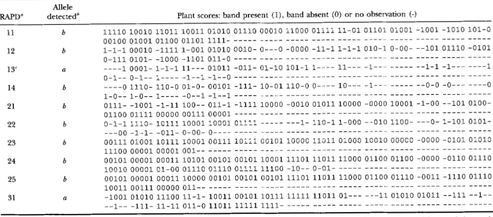
TABLE 1

RAPD data in the backcross progeny of 150 individuals

Allele

RAPD" detectedb Plant scores: band present ( I ) , hand ahsent (0) or no observation {-)

11

12

13'

14

21

22

23

24

25

31

~

b b

a

0-1"0-1"1""-1"1 -1"o """"" """"" """""""""" """""

a

Connecticut King (with alleles represented by a and b at each locus) was crossed with Pirate (with alleles represented by c and d at each locus). Connecticut King was crossed back to one specific F1 hybrid, say with alleles a and c, ab X ac per locus; the cross can he represented by

aabb/bbaa X aaaa/ccccfor segment 1, by aaaaa/bbbbb X aaaaa/cccccfor segment 2 and by ab X ac for segment 3 (see text for further explanation). 'The RAPD band may be present in both parents of the backcross (such an allele is denoted by a ) , only in Connecticut King (allele denoted

'For marker 13, the scores "allele absent" are open to suspicion due to technical problems, and in our analysis presented they were treated

~ ~

RAPD z j is the jth marker on the zth genome segment in Figure 1.

by b) or only in Orlito (allele denoted by c).

as "no observation".

tion can be approximated by the

x:

distribution. The asymptotic distributions are, however, only valid at single positions or intervals. In the preliminary analysis

STRAATHOF et al. (1994) studied 213 RAPDs. The number of plants evaluated per marker varied between 29 and 128 (the average number being 6 4 ) . The linkage map of lily should consist of 12 linkage groups. Unfortu- nately, the RAF'D markers could be integrated only in -100 small linkage groups. Therefore in QTL detec- tion a (probably rather conservative) overall significance level of 5% would be obtained by 0.05 = 1 - ( 1

-

p )

loo with a significance level

p

for each marker test,

ie.,

p

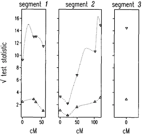
= 0.0005. The critical values in Figure 1 for the nonparametric approach and for the MQM mapping approach would be 3.5 and 4.5, respectively.

QTL likelihood maps are shown in Figure 1, QTL effect maps in Figure 2. Clearly, each of the three putative QTLs has a major effect on the trait. In segment 2

it is indicated that allele a is associated with a higher level of resistance and that allele

a

has a dominant effect on the trait (however see the discussion of "label switching" below). In segment 3 it is indicated that allele a is associated with a lower level of resistance. The situation in segment 1 is more complicated. For the third and fourth marker allele a is associated with a higher level of resistance. For the first and second marker the allelic combination ac is associated with a lower level of resistance. Note that more individuals are genotyped for the first and second marker of segment I than for the third and fourth marker. It would also be interesting to test which alleles have different effects at the most significant QTL positions. For example, at segment 3 we can compare the full three-QTL model with a constrained three-QTL model in which alleles b and c of the QTL at segment 3 have equal effects. The hypothesis of equal effect is not rejected at a 5% signifi-

TABLE 2

Disease scores of the 150 individuals

0 39 -22 -66 18 -89 8 69 -47 41 73 -94 -18 51 -67 -75 -21

*

19 * 137 -21 94

8 67 -80 50 -69 -89 44 36 -67 20 -14 110 30 -40 -39 27 115 44 4 -121 -4

*

-17

22 -22 -44 - 1 1 1 -23 40 44 -56 -111 -66 2 10 75 -81 -98 14 -95 53 47 -21 -31 147 -27

*

70 165 -63 178 -48 19 135 -41 -16 -42 -37 -81 238 79 31 -56 8 178 73 32

19 19 -83 -35 -27 -200 14 75 45 73 -89 14 -52 34 -68 59 74 39 15 39 -19 18 26

67 -16 41 48 -40 -53 24 -53 -42 1 99 -36 40 -49 78 29 -45 80 39 -14 175 45 62

107 81 -67 96 4 -70 -44 77 -60 80 -3 -75

(6)

seqment

1 cM

cM

seament

3 seqment

1

0

cM

0 50

cM

0 50 1 0 0

cM

FIGURE 1.-QTL likelihood maps for Fusarium resistance in lily. A, nonparametric testing (At each marker position the population is divided into two pools on the basis of the absence of presence of the RAPD band; the phenotypic differ- ence between the two pools is tested);

V,

MQM mapping, the full maximum likelihood approach to a three-QTL model ( T o assess the QTL likelihood, a single QTL is moved along the chromosome, while keeping the two other putative QTLs at their nearest marker position obtained in the preliminary analysis; QTL likelihood is calculated at markers positions and in the middle of each marker interval only).

cance level (twice the log-likelihood ratio = 0.1 ) , and alleles b and c could be identical.

The QTL labels ( aa, ab, ac and bc) are indicated in Figure 2, but some labels can still be switched (see also REDNER and WALKER 1984). This can be demonstrated most clearly for segment 3, where the labels aa, ab and ac ( i e . , allele a present) can still be permutated; only the label bc is unique. At segment 2 the labels ab and bc (allele b present) can be switched for all markers at the same time, as well as the labels aa and ac (allele b absent). At segment 1 the labels ab and bc can be switched for the first and second marker, but at the same time the labels aa and ac should be switched for the third and fourth marker.

Compared with the nonparametric approach, our method has several advantages. First, multiple QTLs are fitted simultaneously. This reduces the unexplained variance and therefore improves the power of QTL mapping. Clearly, in our application we have a favorable situation, since the three QTLs explain -85% of the total variance. Second, the phenotypic effects of the four possible genotypes ( aa, ab, ac and bc) at each locus can be unraveled. This also reduces the unexplained variance and increases the power. However, labeling may not be unique. Third, different markers may con- tain different amounts of information about QTLs and our simultaneous analysis of all marker data is more efficient: information from neighboring markers can

seqment

3

0

cM

FIGURE 2.-QTL effect maps produced by MQM mapping. The cross can be represented by aabb/bbaa X aaaa/cccc for

segment 1 , by aaaaa/bbbbb X aaaaa/ccccc for segment 2 and by ab X ac for segment 3 (see also Table 1 1 . In the backcross we have four possible (QTL) genotypes at each locus: aa, ab, ac and be; their estimated effects on the trait are presented at marker positions. In segment 3 the RAPD detects a common allele (allele a )

.

The MQM analysis makes it possible to unravel the effects of genotypes aa, ab and ac (allele a pres- e n t ) . In segment 2 all RAPDs detect an allele originating from the recipient parent (allele b ) . The effects of genotypes

aa and ac (allele b absent) are unraveled as well as those of genotypes ab and bc (allele b present). In segment 1 the situation is more complicated. Note the switch of allele labels

a and b between the second and third marker of parent aabb/ bbaa; therefore in the backcross population the genotype labels aa, ab, ac and be switch to ab, aa, bc and ac, respectively. The effects of the four genotypes are unraveled.

be used to compensate for missing information in the region under study.

DISCUSSION

(7)

now be used in QTL mapping ( HACKETT and WELLER

1995). However, for large progenies with very incomplete marker information, computations in our EM algorithm are not feasible due to the extremely large number of possible complete genotypes. In the present paper, we make our approach applicable to such situations. In each E-step of our new Monte Carlo EM algorithm, complete genotypes are sampled from the conditional probabilities. Monte Carlo samples are easily generated via the Gibbs sampler. Again an artificial data set can be constructed that involves multiple copies of the observed data. Now the number of copies is equal to the number of Monte Carlo runs and the artificial data set consists of all pairs of sampled complete genotypes and observed trait values. It should be mentioned that our approach is not limited to the mapping of QTLs in populations obtained from line crosses. Exten- sions to animal and human pedigree data are possible. Again in each E-step complete genotypes may be sampled from the conditional probabilities by using a Gibbs sampling approach. For instance, the Gibbs sampler proposed by GUO and THOMPSON can be generalized to handle multiple loci in complex human pedigrees. In their paper they considered a single QTL and a single marker, and they used a variance component for QTL background variation. In contrast, we use models for multiple QTLs and multiple markers. Our approach may be more efficient in situations for which a marker map is available.

Here, we also demonstrate that all calculations can easily be done with standard statistical methods and software. There are several advantages: the computer program is general, flexible, short, easy to read and reliable. A serious disadvantage of the Monte Carlo approach, however, is that calculations may be time con- suming. The presence of ( some) closely linked loci represents a worst case: subsequent realizations in the Gibbs sampler may be highly dependent and Monte Carlo realizations should be collected at larger intervals. Nevertheless, we feel that the continuing development of faster computers justifies optimism with respect to the future applicability of Monte Carlo methods in rou- tine genetic mapping.

In our paper we present an extreme application: a backcross between two outbreeding cultivars with many plants that are only partially genotyped for only partially informative markers. Our study clearly illustrates that the full maximum-likelihood approach to multiple- QTL models (MQM mapping) is feasible and informative even with such incomplete data. We should of course strive for the use of more informative markers and completely genotyped progeny. In some applications the data may not be informative enough for proper fitting of models with many parameters. In addition to multiple maxima due to label switching, the log- likelihood may also have many local maxima. Neverthe- less, we believe that our approach shows promise for

tackling the complex problems in both plant and animal and human gene mapping.

The author is greatly indebted to J. M. SANDBRINK, T. P. STRAATHOF and J. M. VAN TWL of the Department of Ornamentals of Centre for Plant Breeding and Reproduction Research, Mogen International N.V. (Leiden, the Netherlands) and Testcentrum Siergewassen B.V. (Hillegom, the Netherlands ) for supplying the data of the example.

LITERATURE CITED

CASELIA, G., and E. I. GEORGE, 1992 Explaining the Gibbs sampler.

FUI.KER, D. W., S. CHERNEY and L. R. CARDON, 1995 Multipoint interval mapping of quantitative trait loci, using sib pairs. Am. J. Hum. Genet. 56: 1224-1233.

Genstat 5 Committee, 1993 Genstat 5 Release 3 Referenw Manual.

Clarendon Press, Oxford.

Guo, S. W., and E. A. THOMPSON, 1992 A Monte Carlo method for combined segregation and linkage analysis. Am. J. Hum. Genet.

51: 1111-1126.

Guo, S. W., and E. A. THOMPSON, 1994 Monte Carlo estimation of mixed models for large complex pedigrees. Biometrics 5 0 417- 432.

HACKETT, C. A,, and J. I. WEILER, 1995 Genetic mapping of quantitative trait loci for traits with ordinal distributions. Biometrics

( i n p r e s s ) .

HALEY, C. S., S. A. KNOTT and J. M. ELSEN, 1994 Mapping quantita-

tive trait loci between outbred lines using least squares. Genetics

JANSEN, R. C., 1992 A general mixture model for mapping quantitative trait loci by using molecular markers. Theor. Appl. Genet.

JANSEN, R. C., 1993 Maximum likelihood in a generalized linear finite mixture model by using the EM algorithm. Biometrics 49:

JANSEN, R. C., 1994 Controlling the type I and type I1 errors in mapping quantitative trait loci. Genetics 138: 871-881.

JANSEN, R. C., and P. STAM, 1994 High resolution of quantitative traits into multiple loci via interval mapping. Genetics 136: 1447-

1455.

JANSEN, R. C., J. W. VAN OOIJEN, P. STAM, C. LISTER and C. DEAN,

1995 Genotype by environment interaction in genetic mapping

of multiple quantitative trait loci. Theor. Appl. Genet. 91: 33- 37.

KONG, A., N. Cox, M. FRICGE and M. IRWIN, 1993 Sequential imputa- tion and multipoint linkage analysis. Genet. Epidemiol. 1 0 483-

488.

LANDER, E. S., and D. BOTSTEIN, 1989 Mapping Mendelian factors underlying quantitative traits using RFLP linkage maps. Genetics

LANDER, E. S., and N. J. SCHORK, 1994 Genetic dissection ofcomplex traits. Science 265: 2037-2048.

MALIEPAARD, C., and J. W. VAN OOIIEN, 1994 QTL mapping in a full-sib family of an outcrossing species, pp. 140-146 in Biometrics in Plant Breeding: Applications of Molecular M a h , edited by J. W. VAN OOIJEN and J. JANSEN. CPRO-DLO, Wageningen, Nether- lands.

REDNER, R. A., and H. F. WALKER, 1984 Mixture densities, maximum likelihood and the EM algorithm. SIAM Rev. 26: 195-239.

STAM, P., 1993 Constructing integrated genetic linkage maps by means of a new computer package: JOINMAP. Plant J. 3: 739-

744.

STRAATHOF, T. P., J. M. VAN TLIYL, B. DEKKER, M. J. M. VAN WINDEN and J. M. SANDBRINK, 1994 Genetic analysis of partial resistance to Fusarium oxysporum in Asiatic hybrid lily using RAF'D markers, in Studies on the Fusarium-lily interaction: a breeding approach,

doctoral thesis by T. P. STRAATHOF. Wageningen Agricultural University, Netherlands.

TANK~LEY, S. D., 1993 Mapping polygenes. Annu. Rev. Genet. 27:

ZEN(:, Z.-B., 1994 Precision mapping of quantitative trait loci. Genet-

Am. Stat. 4 6 167-174.

136 1195-1207.

85: 252-260.

227-231.

121: 185-199.

205-233.

ics 136: 1457-1468.