Quantifying Phylogenetic Conservation in Protein Molecular Evolution

Abstract

FERNANDES, ANDREW DELLANO. Quantifying Phylogenetic Conservation in Protein Molecular Evolution. (Under the direction of William R. Atchley.)

This dissertation examines the problem of quantifying amino acid

conservation in proteins molecular evolution. Ideally, this conservation is quantified by inferring the rate of evolution at each amino acid site of a multiple-alignment. However, current rate-inference methods have three problematic assumptions. The methods assume that (a) the rates of all sites are independent, (b) the rates are drawn from a known prior distribution, and (c) the mean rate across sites is approximately one. The problems are two-fold. First, the assumptions of site-rate independence and known mean rate are contradictory. To see the contradiction, consider a two-site alignment with known rate of ~0.5 at site one. The rate at site two is unknown under the independent-sites assumption, but is ~1.5 by the assumption of known mean rate. Second, if the rates are drawn from a known prior distribution, the assumption of known distribution implies the question “which distribution?”. Previous work has focused only on selecting better families of rate

distributions, often at the expense of additionally parameterizing the

evolutionary model. Herein, I develop a method of inferring rates requiring only the assumption of known mean rate, and not requiring additional parameterization. Thus a model of evolution based on our method is a more general framework for inferring rates than previous work. Since a known mean rate is required to distinguish evolutionary rate from time, our method is arguably the most general possible that allows rate and time to be fully and independently identified. The method is assessed by investigating

Dedication

Biography

Andrew Dellano Fernandes graduated in 1994 from the University of

Acknowledgements

Heartfelt thanks and appreciation go to my advisor, Bill Atchley, for the personal, professional, and financial support he provided.

My spouse, Bonnie Deroo, supported me in untold ways. Words fail me.

Thanks go to advisory committee, including Jeff Thorne, Eric Stone, Steffen Heber, and Charlie Smith, for their thoughts, comments, and time.

Fellow lab-member Kevin Scott kept me statistically honest.

Special thanks are in order to both faculty and staff of the Biomathematics Program and Department of Genetics at the North Carolina State University for providing much-needed support and camaraderie.

Table of Contents

List of Tables ...vi List of Figures ...vii

Preface ...1

Chapter 1

Gaussian Quadrature Formulae for Arbitrary Positive Measures ...3 References ...20

Chapter 2

Detecting Conserved Motifs using Site-Specific

Rate Inference with Objective Non-Informative Priors ...22 References ...64

Chapter 3

Molecular Evolution and Conservation

in the p53 Family of Tumor-Suppressor Proteins...68 References ...106

List of Tables

Chapter 1

Table 1 ...16

Chapter 3

List of Figures

Chapter 1

Figure 1 ...17

Figure 2 ...18

Figure 3 ...19

Chapter 2 Figure 1 ...51

Figure 2 ...52

Figure 3 ...53

Figure 4 ...54

Figure 5 ...55

Figure 6 ...56

Figure 7 ...57

Figure 8 ...58

Figure 9 ...59

Figure 10 ...60

Figure 11 ...61

Figure Supplement A...62

Figure Supplement B ...63

Chapter 3 Figure 1 ...98

Figure 2 ...99

Figure 3 ...100

Figure 4 ...101

Figure 5 ...102

Figure 6 ...103

Figure 7 ...104

Preface

This dissertation examines the problem of quantifying amino acid conservation in proteins molecular evolution. Ideally, this conservation is quantified by inferring the rate of evolution at each amino acid site of a multiple-alignment. However, current rate-inference methods have three problematic assumptions. The methods assume that (a) the rates of all sites are independent, (b) the rates are drawn from a known prior distribution, and (c) the mean rate across sites is approximately one. The problems are two-fold. First, the

assumptions of site-rate independence and known mean rate are contradictory. To see the contradiction, consider a two-site alignment with known rate of ~0.5 at site one. The rate at site two is unknown under the independent-sites assumption, but is ~1.5 by the assumption of known mean rate. Second, if the rates are drawn from a known prior distribution, the

assumption of known distribution implies the question “which distribution?”. Previous work has focused only on selecting better families of rate distributions, often at the expense of additionally parameterizing the evolutionary model.

Herein, I develop a method of inferring rates requiring only the assumption of known mean rate, and not requiring additional parameterization. Thus a model of evolution based on our method is a more general framework for inferring rates than previous work. Since a known mean rate is required to distinguish evolutionary rate from time, our method is arguably the most general possible that allows rate and time to be fully and independently identified. The method is assessed by investigating conservation in the Myc, Max, and p53 transcription-factor families.

clades. Second, some conservation measures did not correct for amino acid physiochemical similarity and evolutionary exchangeability. Thus the small change of leucine to isoleucine was given the same weight as the large change of phenylalanine to proline. The only measure of conservation incorporating phylogenetic and amino acid similarity data was evolutionary rate, as given in standard stochastic models of protein evolution. Unfortunately, estimating rates through these models used the three assumptions of site independence, known

distribution, and fixed mean rate, as described above. Chapter 2 describes the methods I developed to avoid these assumptions and the problems that they create.

The process of developing this method required the many computations of likelihood integrals. Calculation of these integrals consumes the majority of computer time in many molecular evolution studies, including ours. Evolutionary biologist Joseph Felsenstein noted in 2001 that the numerical integration technique of Gaussian quadrature could be used to significantly speed up evaluation of these integrals. Unfortunately, integration schemes for only a few specific forms of the integral were known. Chapter 1 presents work extending the evaluation of likelihood integrals by Gaussian quadrature to arbitrary integrands. It has been reviewed by Felsenstein and has been accepted for publication in Evolutionary

Bioinformatics Online.

Therefore this dissertation is presented in reverse-telescopic order: investigations of the p53 family begat investigations of site-specific rate inference. Rate inference in turn begat questions regarding the evaluation of likelihood integrals. First, I solved the problem of integration. Next, I completed the work on rate inference. Finally, our results were applied to the p53 family.

Chapter 1

Gaussian Quadrature Formulae for

Arbitrary Positive Measures

(Arbitrary Gaussian Quadrature Formulae)

Andrew D. Fernandes1,2,4 & William R. Atchley1,2,3

1_{Graduate Program in Biomathematics} 2_{Center for Computational Biology}

3_{Department of Genetics} North Carolina State University

Raleigh, NC 27695-7614

Abstract

We present computational methods and subroutines to compute Gaussian quadrature integration formulas for arbitrary positive measures. For expensive integrands that can be factored into well-known forms, Gaussian quadrature schemes allow for efficient evaluation of high-accuracy and -precision numerical integrals, especially compared to general ad hoc schemes. In addition, for certain well-known density measures (the normal, gamma, log-normal, Student’s t, inverse-gamma, beta, and Fisher’s F) we present exact formulae for computing the respective quadrature scheme.

Availability: Source code is freely available online as a C-linkable ISO C++ library under a BSD-style license from http://www.fernandes.org/gaussqr. The library may be built using single, double, or extended precision

arithmetic.

Motivation

This paper is concerned with the efficient and accurate calculation of likelihood integrals of the form

Pr

(

H D

)

Pr

( )

D h Pr

( )

h hH

dh, (1)

through the construction of a Gaussian-type quadrature scheme that is optimized specifically for the known prior distribution Pr

( )

h . Our specific motivation stems from studies in the molecular evolution of protein sequences where it is important to take variation of

evolutionary rates among sites into account when inferring phylogenies. In the context of this specific problem, both Felsenstein (2001; 2004) and Mayrose et al. (2005) pointed out that Gaussian quadrature formulae can be used to provide more accurate and more rapidly

convergent numerical integration methods than the more common “equal percentile” method of Yang (1994). Unfortunately, Gaussian-type quadrature formulae have only been derived for a relatively small number of prior distributions. In the context of molecular evolution, the two most common priors are the gamma and log-normal distributions. Gaussian quadrature formulae for the gamma distribution are already known as “Generalized Gauss-Laguerre” quadrature (Felsenstein 2001), although admittedly the mathematical similarity between these schemes is not obvious with the usual formulation of Gauss-Laguerre quadrature. Thus their equivalence is generally not appreciated. Unfortunately, until now explicit Gaussian quadrature formulae were not available for log-normal (or other) priors commonly used in computational biology.

The purpose of this paper is to provide an efficient and rapid algorithm with

Problem Statement

We wish to find a set i=0,1, 2,…,

(

n1

)

of weights wi and abscissae xi such that the approximation

w x

( )

f x

( )

a

b

dx wi f x

( )

i

i=0 n1

(2)

is exact whenever f is a polynomial of degree 2n1 or less, and w x

( )

is a known “weight function”. In our case w x

( )

represents the positive density measure of our prior likelihood.

A good and complete modern reference covering the theory of Gaussian (and related) types of quadrature rules can be found in Gautschi (2004). If f is expanded as a polynomial series,

inspection suggests that any quadrature scheme will depend on the raw moments of w x

( )

.

Indeed, defining the (real) inner product

f g =

f x

( )

g x

( )

w x

( )

dx, (3)

it is well known that there always exists a set of polynomials, orthogonal with respect to this inner product, such that

p₁=0, p0 =1

pi+1

( )

x =

(

xai

)

pi

( )

x bipi1

( )

x , i=0,1, 2,…

(4)

and where the recurrence coefficients ai and bi can be calculated explicitly from

ai =

xpi pi

pi pi

, i=0,1, 2,…

bi =

pi pi

pi1 pi1

, i=1, 2,…

(5)

J =

a0 b1

b1 a1 b2

b2

b_n2

b_n2 a_n2 b_n1 b_n1 a_n1

. (6)

The desired abscissae x_i are then equal to the eigenvalues of J , and the desired weights are given by the relationship

wi =b0qi,0

2 _{, (7)}

where qi,0 is the first component of the normalized eigenvector qi of matrix J.

Solution Methods

Formulae are known that explicitly express the recursion coefficients aj and bj in terms

of the raw moments of w. Unfortunately, these explicit representations are extremely ill-conditioned and thus are not usable even for “well behaved” weight functions or quadrature schemes of fairly low order n. If the integrals of Equation (5) can be calculated efficiently and accurately, Stieltjes’ Procedure calculates the recursion coefficients via iterative application of Equations (4) and (5) forming the sequence

p₁,p0

{

}

{

a0,b1

}

{ }

p1

{

a1,b2

}

{ }

p2 . Although better behaved than explicit computation, Stieltjes’ Procedure also tends to be moderately ill-conditioned (Press,

heuristic approximation of the moments of w x

( )

. Forming such an approximation may be as

or more difficulty than solving the original problem.

Recently, a general-purpose and unconditionally stable algorithm to calculate Gaussian weights and abscissae for any positive measure has been proposed (Gander and Karp 2001). The method is based on the observation (Boley and Golub 1987) that the discrete measure

m

( )

x = i i=0 m1

(

x_i

)

(8)

can have its weights and abscissae assembled into a sparse matrix

Wm =

1 0 1 m2 m1

0 1

1 2

m2 m2

m1 m1

(9)

that is orthogonally similar to the Jacobi matrix

J_m =

1 b0

b₀ a₀ b₁

b₁ a₁ b₂

b₂

bm2

bm2 am2 bm1

bm1 am1 , (10)

where b₀ is the _m-measure of the entire domain of_m. Gander and Karp showed that if a

sequence of discrete measures given by Equation (8) converged to a given continuous measure such that lim

exploited several years before in the ORTHPOL software package (Gautschi 1994). A re-implementation, modernization, and modification of some of Gautschi’s algorithms form the core of our work. To continue, given Jm, standard eigen-decomposition algorithms for

symmetric tridiagonal matrices can be used to compute the Gaussian quadrature weights and abscissae for the given weight function. In summary, the weights and abscissae of an

arbitrary positive measure w x

( )

can be as determined by first finding a discrete m

( )

x that

approximates w x

( )

“well enough”, using the Lanczos reduction algorithm to transform

WmJm, concomitantly obtaining the recursion coefficients

{

ai,bi

}

, and then

eigen-decomposing Jm to determine the final weights and abscissae

{

xi,wi

}

via Equation (7).

Algorithmic Details

The implementation details for the overall process, starting from a given weight function and ending with a set of Gaussian quadrature weights and abscissae, are best elucidated by a

worked example. Assume we are given the weight function w x

( )

ex_,

x0, where we do

not know the normalization constant 1

w x

( )

dx and do not recognize ex _{as the weight}

function for the well-known Gauss-Laguerre quadrature scheme. Our first step is to select a

sequence of measures, as per Equation (8), that converges to the measure ex dx. Following

Gautschi (1994), we use a classical numerical integration scheme to approximate

w x

( )

dx,

namely the Fejér Type-2 integration rule (Gautschi originally used the Fejér Type-1 rule). Fejér integration rules are very similar to the well-known Clenshaw-Curtis integration rules over the domain z

[ ]

1,1 . However, the Fejér rules are open-ended, do not require

evaluation at the domain endpoints, and are therefore more suitable for measures with non-compact support. Fejér Type-2 rules also have an efficiency advantage over the Type-1 rules in the fact that the n-point Type-2 abscissae are an interleaved subset the

(

2n+1

)

-point

2006), allowing a large number of points to be efficiently utilized in approximating

w x

( )

dx. The supplied subroutine fejer2_abscissae calculates the required abscissae and integration weights

{ }

zi,qi for a given number of abscissae i=0,1, 2,…,

(

m1

)

. The

transformation g z

( )

=

(

1+z

)

1z

(

)

is used via the subroutine map_fejer2_domain to map

z 1,1

(

)

x

( )

0, and change the variable of integration such that

ex

0

dx= eg z( ) g z

( )

1

+1

dz, giving the final abscissae and weights

{

i,i

}

for Equation (9),

where i =g z

( )

i and i =qiw g z

(

( )

i

)

g z

( )

i . Note that the subroutine map_fejer2_domain

is capable of mapping the Fejér interval to other arbitrary finite and non-finite domain intervals in addition to the particular transformation g z

( )

utilized here.

The tridiagonalization of Wm in Equation (9) to Jm in Equation (10) can be accomplished

by using the subroutine lanczos_tridiagonalize, a subroutine that exploits the sparsity

structure of Equation (9) via the Lanczos algorithm (Golub and Van Loan 1996) for efficient tridiagonalization. Lastly, the eigen-decomposition of Jm in Equation (10) and subsequent

calculation of the final Gaussian quadrature rule for w x

( )

via Equation (7) is accomplished by use of the subroutine gaussqr_from_rcoeffs, where the eigen-decomposition is performed using a modified implicit-shift QL algorithm. Note that the coefficient b0 returned from

lanczos_tridiagonalize estimates

w x

( )

dx for the given m. Thus, we can set b0 =1 prior to

calling gaussqr_from_rcoeffs to normalize w x

( )

without explicitly knowing or calculating

the actual normalization coefficient. In many cases, this can significantly speed up the calculation of w x

( )

. For common distributions such as the normal, gamma, log-normal, and others, the utility function standard_distribution_rcoeffs is supplied to compute recursion coefficients directly.

Lastly, we must ensure that m is large enough so that m

( )

x approximates w x

( )

points

{

xi,wi

}

converge. The subroutine relative_error computes the maximum relative error

between its two vector arguments. Since wi is guaranteed to be positive for all non-negative

measures w x

( )

, it suffices (and simplifies matters) to verify convergence of wi without explicit regard to the convergence of xi.

Implementation Details

In using the subroutines presented, there are a few subtleties in the overall procedure that can be exploited in order to address non-standard situations or increase computational efficiency. First, we note that the discrete measure denoted by Equation (8) can be used to approximate any finite union of disjoint intervals. For instance, if we wished to use the (admittedly contrived) implicit weight function

w x

( )

e x

, 0x<1 1 x2

, 1x

(11)

over support 0x. Our subroutines could be applied twice, once for each continuous

interval, yielding two discrete-measure approximations, each with approximate normalization consonant. The two discrete measures could then be combined into a set of abscissae and

weights

{

i,i

}

that would then be subject to the Lanczos tridiagonalization procedure in

order to determine the recursion coefficients of Equation (11). Note that the normalization of Equation (11) is computed “on the fly” and therefore allows great flexibility in choosing the weight function w x

( )

. Furthermore, note that the example weight function of Equation (11)

is not even continuous at x=1.

Second, we note that computing an m-node Fejér Type-2 integration scheme is done by performing a real inverse fast Fourier transform of size

(

m+1

)

. Although the subroutine

supplied is capable of computing inverse Fourier transforms of almost arbitrary size, the transform is efficient only if

(

m+1

)

has divisors from the set

{

2, 3, 4, 5

}

. To further increase

zi =cos i+1

(

)

m+1

, i=0,1,…,

(

m1

)

, (12)

implying that an m₁-point and m₂-point integration scheme will share common abscissae if

m1+1

(

)

and

(

m2 +1

)

have a common divisor. Having common abscissae imply that

previously computed values of w g z

(

( )

i

)

could be reused as m increases, thus increasing the

efficiency of approximating w x

( )

. Therefore the recommended sequence of m for

fejer2_abscissae follows

{

3, 7,15, 31, 63,…

}

. For very simple, well-behaved weight

functions, it may be preferable to simply use m of a few hundred or few thousand, and not worry excessively about convergence when m is small. Such an approach may be indicated when pre-computing quadrature schemes for a parameterized family of weight functions; the shape parameter of the unit-mean gamma distribution, for example. Rather than determining quadrature points for every desired shape parameter, it may make more sense to pre-compute weights and abscissae as functions of the shape parameter at particular parameter values, and then interpolate a quadrature scheme for all “in-between” parameter values. Obviously, Fejér nodes and weights can be pre-computed as well.

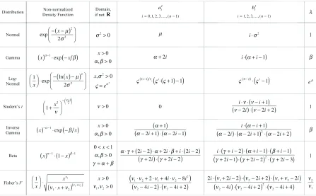
There may be situations where it is useful to know the analytic form of a particular weight function’s recursion coefficients. In particular, well-known density functions can often have their recurrence relationships determined by Stieltjes’ Procedure, and a

representative sample of such is shown in Table 1. Recursion coefficients computed from this table can be supplied directly to subroutine gaussqr_from_rcoeffs, although better numeric stability may be achieved by approximating these densities via standard_distribution_rcoeffs. Note that Gaussian quadrature schemes may not exist for all distributions at all parameter values. In these cases, non-existence of the quadrature scheme is due to the non-existence of the distribution’s relevant higher-order moments. In any case, caution should be exercised in utilizing Table 1 for these distributions lest numerical truncation error inadvertently become too great. Lastly, as Table 1 shows, it is often possible to extract a common factor from the recursion coefficients. Such a common factor merely scales the eigenvalues of Jm while

We conclude with a reminder that our choice of the Fejér Type-2 integration points for computing the approximation lim

mm

( )

x =w x

( )

is quite arbitrary, and other integration schemes may be more appropriate given a different family of weight functions. For instance, a simple 1 m “equal-percentile” approach, reminiscent of Yang (1994), may be more

efficient than a Fejér-like scheme for weight functions with numerous sharp peaks. Further, rational-quadrature schemes may be a better choice for measures with poles near the

measure’s support (Gautschi 1999; Weideman and Laurie 2000; Van Deun, Bultheel et al. 2006). In any case, the Fejér Type-2 scheme utilized here should prove adequate for most common weight functions utilized in likelihood calculations today.

Usage Guidelines

Two approximations must be made to construct a set of quadrature abscissae and weights. First, the number of discrete points that will be used to approximate the weight function must be chosen. Second, the number of quadrature points to compute the final likelihood integral must be chosen. In this section, we provide guidance on how to select the appropriate number of points in each case.

First, when approximating w x

( )

by a discrete measure, we exploit efficiencies inherent in the FFT and sparsity structure of matrices W_m and J_m to quickly and efficiently

approximate w x

( )

with thousands (1023, 2047, or more) points. For example, using 1023 points to approximate a standard N

( )

0,1 distribution results in quadrature coefficients, correct to within one part in 21015 (the limit of machine precision), to be calculated in negligible time compared to all but the most trivial phylogenetic likelihood calculations.

Guidance for the second case, the number of quadrature points to use, is more difficult to give because of the main convergence property of Gaussian quadrature: the rate of

guidance on picking the number of quadrature points for a particular integrand may come from trial and error: keep increasing the number of points until numerical convergence seems to be achieved. This empirical “try it and see” approach has been utilized by Yang (1994), Mayrose et al. (2004), among others and is commonly advised.

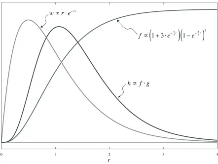
In an effort to provide a more concrete example of how Gaussian quadrature fares in a sample integrand from molecular evolution studies, consider one site of a four sequence alignment where every nucleotide is different (one each of A, C, G, and T), and we know a priori that all four sequences share an unknown common ancestor one time unit in the past. Assuming a normalized Jukes-Cantor (1969) model of evolution yields a likelihood function of

f r

( )

(

1+3e43r

)

(

1e43r

)

3

(13)

for a given evolutionary rater. We assume unit-proportionality for convenience. Further

assuming that rates are distributed according to a unit-mean Gamma distribution with

coefficient of variation 2 results in a weight function of

w r

( )

=4re2r_{. (14)}

The likelihood of our data given our model can then be calculated analytically, resulting in

h r

( )

dr

0

= 30080

533610.5637076, (15)

where

h r

( )

=w r

( )

f r

( )

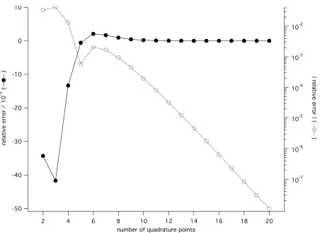
. (16)

A graph depicting the relative shapes of f , g, and h is shown in Figure 1. A plot of the

relationship between the number of quadrature points and the relative error of the integral in Equation (15) is shown in Figure 2. Seven quadrature points result in a relative error of about

0.15%, and twenty points result in a relative error of about 1.1106_{%. Note that seven or}

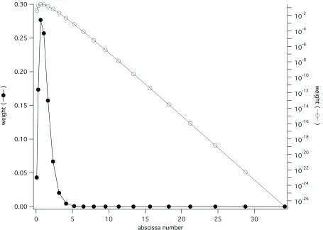
A detailed examination of the twenty-quadrature point case shows an interesting

optimization that applies to likelihood functions such as Equation (13), where the likelihood approaches a constant value as its argument approaches infinity. Recall that Gaussian

quadrature schemes are designed to optimally integrate polynomials p x

( )

, and that complex

analysis tells us that for polynomials, p x

( )

as x . For w x

( )

p x

( )

to be

integrable, w x

( )

0 relatively rapidly as x . Therefore we expect the quadrature

weight w_i to rapidly become very small as the magnitude of its respective abscissa x_i

increases. An illustration of the magnitudes of

{

xi,wi

}

for a twenty-point quadrature scheme

for our h r

( )

example, above, is shown in Figure 3. Note that after the first ten to twelve

abscissae have been summed, the contribution of the remaining eight to ten points will be

negligible; the integration scheme assumes that f r

( )

will be polynomially large when in fact

it is almost constant. Thus we can gain the accuracy benefits of using a twenty-point

integrator while incurring the cost of only ten evaluations of f r

( )

.

Acknowledgements

Table 1

Exact recursion coefficients for selected probability distributions. For Equations (6) and (7), we scale the recursion coefficients such that ai = ai and bi =

2

Figure 1

Figure 2

Figure 3

Gaussian quadrature weights and abscissae for n=20 points for the sample molecular

References

Boley, D. and G. H. Golub (1987). "A survey of matrix inverse eigenvalue problems." Inverse Problems 3(4): 595-622.

Felsenstein, J. (2001). "Taking Variation of Evolutionary Rates Between Sites into Account in Inferring Phylogenies." Journal of Molecular Evolution 53(4 - 5): 447.

Felsenstein, J. (2004). Inferring Phylogenies. Sunderland, MA, USA, Sinauer Associates.

Gander, M. J. and A. H. Karp (2001). "Stable computation of high order Gauss quadrature rules using discretization for measures in radiation transfer." Journal of Quantitative Spectroscopy & Radiative Transfer 68(2): 213-223.

Gautschi, W. (1994). "Algorithm 726: ORTHPOL - A Package of Routines for Generating Orthogonal Polynomials and Gauss-Type Quadrature Rules." ACM Transactions on Mathematical Software 20(1): 21-62.

Gautschi, W. (1999). "Algorithm 793: GQRAT - Gauss quadrature for rational functions." ACM Transactions on Mathematical Software 25(2): 213-239.

Gautschi, W. (2004). Orthogonal polynomials: computation and approximation. New York, Oxford University Press.

Golub, G. H. and C. F. Van Loan (1996). Matrix computations. Baltimore, Johns Hopkins University Press.

Jukes, T. H. and C. R. Cantor (1969). Evolution of protein molecules. Mammalian Protein Metabolism. H. N. Munro. New York, Academic Press. 3: 21-132.

Mayrose, I., N. Friedman, et al. (2005). "A Gamma mixture model better accounts for among site rate heterogeneity." Bioinformatics 21: 151-158.

Mayrose, I., D. Graur, et al. (2004). "Comparison of site-specific rate-inference methods for protein sequences: Empirical Bayesian methods are superior." Molecular Biology and Evolution 21(9): 1781-1791.

Press, W. H., S. A. Teukolsky, et al. (1997). Numerical recipes in C: The art of scientific computing. Cambridge, Cambridge University Press.

Van Deun, J., A. Bultheel, et al. (2006). "On computing rational Gauss-Chebyshev quadrature formulas." Mathematics of Computation 75: 307-326.

Weideman, J. A. C. and D. P. Laurie (2000). "Quadrature rules based on partial fraction expansions." Numerical Algorithms 24(1 - 2): 159.

Chapter 2

Detecting Conserved Motifs using Site-Specific Rate

Inference with Objective Non-Informative Priors

(Detecting Conserved Motifs using Site-Specific Rate Inference)

Andrew D. Fernandes1,2,4 & William R. Atchley1,2,3

1_{Graduate Program in Biomathematics} 2_{Center for Computational Biology}

3_{Department of Genetics}

North Carolina State University Raleigh, NC 27695-7614

4_{Corresponding Author}

Abstract

Motivation: The detection of conserved protein sequence motifs depends

critically on the precise definition of “conservation” used. Current measures of conservation suffer from one or more of three flaws: they may not account for similarities or differences among amino acids, they may not correct for the phylogenetic correlation among the given sequences, or they may depend to an unknown extent on a parameterized ad hoc prior distribution. We propose a novel method of detecting conserved motifs that does not suffer from these flaws. The method first infers site-specific rates of evolution using a class of objectively non-informative rate priors, and then associates low rates of evolution with conserved, and hence functionally or structurally important, sites. An extensive analysis of conservation within proteins from the Myc-Max transcription factor family is given, with detailed comparison to previous methods of detecting conservation.

Results: Given a sequence alignment, an estimate of the alignment’s

phylogeny, and a model of amino acid substitution, our method efficiently estimates the rate of evolution at each site using a prior chosen from a class of objectively non-informative rate priors. While generally superior to other methods of detecting conservation, the results are critically dependent on the quality of the sequence alignment analyzed.

Contact: Andrew D. Fernandes [email protected]

William R. Atchley [email protected]

Keywords: site-specific rate variation; protein evolution; likelihood;

Introduction

In proteins, the rate of evolution at each residue site is expected to vary according to the specific selective constraints at that site. Sites that are under strong selective constraints should be relatively highly conserved, while sites under lesser selective pressure should be more variable, with the observed rate corresponding to the level of purifying selection at that site (Kimura 1983). Therefore conserved sites are often strongly suggestive of structural or functional importance. Such conserved residues may be involved ligand binding, secondary or tertiary structure conformation, DNA binding, protein folding, or protein-protein

interactions. A relatively small, contiguous set of relatively conserved sites that accurately identify a specific set of homologous proteins, such as the basic Helix-Loop-Helix (bHLH) transcriptional regulators, is called a sequence signature or sequence motif (Atchley, Terhalle et al. 1999; Atchley and Fernandes 2005). This paper is concerned with the problem of determining which sites, given an aligned set of protein sequences and their associated phylogeny, should be denoted as being conserved and are therefore candidate sequence motifs.

Previous Work

Although many different site-specific conservation scores for multiple alignments have been proposed in the past (reviewed in Valdar 2002), none of these methods make full use of the information contained in the phylogenetic tree that relates the sequences, or the

evolutionary exchangeability of different amino acids. A conservation score based on entropy that incorporated phylogenetic information was introduced by Wollenberg and Atchley (2000), but this score did not account for the effective similarity (such as isoleucine and leucine) or dissimilarity (such as proline and tryptophan) of individual amino acids. More recently still, at least two independent frameworks, namely MrBayes (Ronquist and

conversely, higher rates indicate proportionally less conservation at that site. Both of these programs infer evolutionary rates using a Bayesian framework in essentially similar manners. For brevity, we will describe the general procedure utilized by these programs to infer rates, ignoring minor details where they differ.

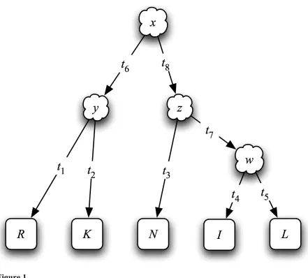
Assume an alignment A and phylogenetic tree T such that site i of the alignment,

denoted byAi, as shown in Figure 1. Branch lengths of the phylogenetic tree represent the

average number of amino acid replacements between nodes of each branch, averaged across

all sites. The site-specific rate ri indicates how quickly site i evolves relative to the average.

Therefore, following standard likelihood calculations, we can write

P A

(

i T,ri

)

= P x

( )

P y x,r

(

it6

)

P R y,r

(

it1

)

P K y,r

(

it2

)

y

x

P z x,r

(

_it₈

)

P N z,r

(

_it₃

)

P w z,r

(

_it₇

)

P I w,

(

r_it₄

)

P L w,

(

r_it₅

)

w

z

, (17)

where P x

( )

denotes the background (prior) probability of amino acid x, and P y x

(

,ritj

)

denotes the probability that amino acid x will be replaced by amino acid y along a branch

length of tj if the site is evolving at rate ri. In practice, Felsenstein’s (1981) post-order tree

traversal algorithm is used to calculate this likelihood efficiently. If we use a time-reversible model of amino acid substitution, as is usually the case, the root node could be placed anywhere on the tree without changing the computed likelihood. To infer rates given the data, Bayes’ Theorem can be used to set

P r

(

_i T,A_i

)

P A

(

_i T,r_i

)

P r

( )

_i . (18)

Thus we are left with the necessity of specifying the prior density P r

( )

i for each of the rates.

Gamma distribution with shape parameter >0 and inverse-scale parameter has mean

and variance 2_{. Setting} = _{yields a distribution of mean one and variance}

1 2, with the shape of the density being determined by alone. When >1 the density is

bell-shaped and unimodal; as gets larger there is progressively less rate heterogeneity and rates tend to be progressively closer to one. When 1 the density is L-shaped in the manner of the Exponential distribution; as shrinks the density becomes progressively more skewed and obtains a wider range of rate heterogeneity.

Once a rate prior has been selected, the mean and variance of the posterior rate distribution can now be calculated via

Er_i A,T = r_iP r

(

_i A_i,T

)

0

dr_i =r_i

riP A

(

i ri,T

)

P dr

( )

i

0

(19)

and

Varr_i A,T =

(

r_i r_i

)

2P r

(

_i A_i,T

)

0

dr_i

(

ri ri

)

2

P A

(

i ri,T

)

P dr

( )

i

0

. (20)

The integrals given in Equations (19) and (20) are analytically intractable and must be approximated by an appropriate numerical scheme. The most popular is the “equal

probability discretization” quadrature scheme introduced by Yang (1994) that approximates the integral

f x

( )

dx x

X

wif x

( )

i i=1

m

(21)

for some discrete set of knot points xi X and a given set of weights wi. Specifically,

Yang’s scheme partitions X into m equal-percentile sets, assigns x_i to be the mean of

integration technique of Gaussian quadrature yields a higher accuracy result for

comparatively fewer evaluations off x

( )

i . Gaussian quadrature uses a somewhat involved

procedure to find a set of knots and weights for Equation (21) that yields numerically exact results for a large class of functions. Further details of constructing Gaussian quadrature schemes for arbitrary functions f can be found in Fernandes and Atchley (2006).

Finally, if alignment A consists of n sites, the likelihood of a given set of rates

r1,r2,…,rn

{

}

can be computed by the relationship

P r

(

1,r2,…,rn A,T

)

= P r

(

i Ai,T

)

i=1

n

P A

(

i ri,T

)

P r

( )

i i=1

n

, (22)

from which summary statistics can be computed. This is termed the Empirical Bayesian (EB) approach for inferring site-specific rates. The term “empirical” is used because the shape parameter of the Gamma distribution rate prior is generally unknown and hence must be estimated from the data (Robbins 1956; Leonard and Hsu 2001). Because of the difficulty of choosing a prior distribution that is optimal from everyone’s differing points of view, it has been argued that no prior for the rates should be assumed, the equivalent of assuming

P r

( )

i =1. This choice of prior is termed the Laplace prior and implies that Equation (22) can

now be interpreted in a Maximum Likelihood (ML) framework if desired. In the ML interpretation, the best estimates rˆ_i for the rate parameters r_i are

ˆ

ri =arg max

r_i P A

(

i ri,T

)

, (23)

with related significance and variance estimates coming from classical ML theory. In fact, the original formulation of rate4site (see Pupko, Bell et al. 2002) used an ML framework to infer evolutionary rates. They found that the lack of a rate prior could, in rare circumstance, lead to the case where rˆ_i if an alignment site had all different amino acids at that site.

inference; so much so, in fact, that the EB approach was recommended for all general use. In some sense, the superiority of Bayesian over ML methods in the context of rate inference was anticipated by Felsenstein (2001) who pointed out that a model with a separate rate for each site would result in the number of parameters increasing at the same pace as the increase in alignment length, causing the likelihood methods to lose their property of consistency. Thus many of the asymptotic convergence properties that ML methods rely on would no longer hold, implying that much of the standard ML machinery would be invalidated. Note that in a Bayesian context, estimating too many parameters from the data results in

(potentially drastic) variance inflation, but does not invalidate the analytical context on which the estimation is based.

Criticisms of EB Rate Inference

Having described the EB methodology for rate inference, we turn now to criticisms of this methodology. Our goal is to formulate a method of rate inference that addresses these criticisms and ameliorates the difficulties that arise from them. The criticisms we present below are not intended to imply that EB rate inference is somehow incorrect. Rather, we hope to merely highlight the major assumptions and approximations inherent in EB rate inference, pointing out why the criticism is significant. After all, there is a large body of established literature that uses EB methods very similar to what we have described, and uses them with notable success. Any proposed new methodology would be suspect if it produced results that were not consistent with this body of previous work.

The Gamma Distribution

The first criticism involves the ad hoc selection of the Gamma (or Gamma-like)

al. 1995), a mixture of Gamma distributions can be utilized (Mayrose, Friedman et al. 2005), or other more general parameterized distributions (Kosakovsky Pond and Frost 2005) can be used. Generally speaking, the more flexible the parameterized family of distributions utilized for a prior, the more likely that the prior will capture the “true” distribution of rates that are present, but unobserved, in the data.

Unfortunately, it is difficult to determine when the rate prior has been made flexible enough to “correctly” model the data. For instance, we could utilize Bayes factors (Robert 2001) or Akaike’s Information Criterion (AIC, 1974) to select between two different

hypothetical rate priors: the first consisting of a Gamma distribution, the second consisting of a Gamma distribution augmented with a proportion of invariant sites. The latter model is clearly more flexible than the former and may well better model the existing rate

heterogeneity. However, for a shape parameter greater than one, for example, both models assume that large rates are roughly exponentially less likely than lower rates. If this assumption is not true and a relatively large fraction of sites are evolving quickly, then the posterior rate distribution may be significantly yet undetectably biased due to the fact that neither prior adequately captures the true behavior of the rate distribution.

Distribution Parameters

Influence of the Prior

If an empirical prior is used, how can we know whether the data or the prior dominates the posterior? One simple idea is to use two alternative priors and check the resultant posteriors for agreement. But this procedure is rather indirect and, moreover, may be more informative about the two alternative priors than about the data. In some ways this restates the previous two sections that criticized both the use of the Gamma distribution and requirement for parameter estimation. Our point here is deeper, however. Given any set of alternative priors, how can we determine which one, if any, is the most appropriate?

The field of objective Bayesian analysis attempts to answer this question by turning the question on its head. Rather than verifying what comes out of an analysis, what if we are more careful about what goes into it? If the prior is designed to satisfy a rigorous and

objective set of criteria that quantify our prior ignorance about the parameter in question, it is logical to assume that we have a better understanding of how the prior has influenced the posterior. An analogous situation is the observation that, by using better ingredients, we will likely bake a better cake. A prior that is designed to satisfy such criteria is termed an

objective prior (Berger 2006). An excellent review of the selection of prior distributions by formal rules has been written by Kass and Wasserman (1996). Note that objective priors should not be automatically interpreted as being automatically “better” than either subjective or empirical priors. Rather, a prior is deemed “objective” when it has been chosen to satisfy objective criteria that capture, in a rigorous way, the precise nature of our ignorance. One may thus object to the criteria, but not the resultant prior.

Since rates are by definition non-negative any reasonable rate prior should have support of the non-negative real numbers and be integrable. Although improper (non-integrable) priors are often used in Bayesian analysis, their use in likelihood calculations as per Equation (17) results in improper posteriors. Given this restriction, relatively few

posterior. Unfortunately, it is unclear how to construct an objective prior that could be utilized within in the current framework for rate inference.

Reparameterization Invariance

One criterion that many feel is important for a Bayesian prior is re-parameterization invariance (Robert 2001). Reparameterization invariance means that no matter how our parameter of interest is measured, the prior always expresses the same equivalent belief. Stated mathematically, a prior density h is termed invariant if

h

( )

=h g

(

( )

)

g

( )

(24)

whenever g is a one-to-one differentiable transformation satisfying

f x

( )

= f g x

(

( )

g

( )

)

g x

( )

x (25)

for all x and , where f x

( )

is the likelihood density. That is, it should make no

difference whether evolutionary change is measured as a rate parameter (“average amino acid replacements per unit time”) or its reciprocal, a time parameter (“average time per amino acid replacement”). Both quantities represent a measure of the same physical quantity, and therefore an analysis performed on one parameter should yield identical inferences to an analysis of the other. Unfortunately, the Gamma-family of distributions does not satisfy the invariance principle. Furthermore, given the described rate inference framework, it is not clear how to construct an invariant prior for site-specific rate parameters.

Confounding with Time

Perhaps the most serious criticism against the current EB rate inference method is the mathematical confounding of evolutionary rates with divergence times between the nodes of the phylogenetic tree. Thus, there is no way to distinguish between (a) doubling all of the inferred rates and (b) halving all of the tree’s branch lengths. Unfortunately, lack of

other rates. Generally, rates are relative to a mean rate of one. Thus, a rate of two indicates amino acid replacement is twice as fast as the average, a rate of half indicates a rate half the average. To interpret rates as relative measures, the rate prior distribution is usually

constrained to have a unit mean to de-confound rate and time.

Unfortunately, constraining the prior alone is insufficient because it does not equivalently constrain the posterior. The posterior rate distribution remains with rate and time

confounded. For example, suppose we have data x consisting of m samples of a Normal

distribution that has known variance 2 _{and unknown mean} μ_{. To estimate}

Eμ x,2 in a

Bayesian framework requires a prior distribution for μ. We assume the prior to be Gaussian

such that μN μ0,0 2

(

)

, where the mean μ0 and variance 0

2 _{of the prior are arbitrary}

hyperparameters. Setting

P

(

μ x,2

)

P x

(

μ,2

)

P

( )

μ (26)

yields

μ x,2 N μ*,* 2

(

)

, (27)

where

μ* =* 2 μ0

0 2 + mx 2

and *

2 ₌ 1

0 2 + m 2 1 . (28)

Notice that no matter how tight the prior’s variance ₀2 _{nor the location of the prior’s mean}

μ0, given enough samples eventually *

2 2

m0 and μ*x. Restricting the prior of

Why is confounding a problem? Consider the case where we hold the alignment A and

tree topology T fixed but we wish to estimate not only the site-specific rates r, but the

tree’s branch lengths t as well. Then

P r,

(

t A,T

)

P A,T r,

(

t

)

P r,

( )

t

=?P A,T r,

(

t

)

P r

( )

P t

( )

(29)

in the current framework. However, if rates and times are confounded, it is impossible to

construct a meaningful prior for t, as P r

( )

,t cannot be separated into P r

( )

P t

( )

. Of

course, there is no a priori reason that rates and times be separable, but if they are not

interpretation becomes very difficult. For instance, consider the simple problem of

computing the conditional probability P r t

( )

. Unless the probabilities of r and t are

separable, such a seemingly simple statement is meaningless and cannot be computed. This is a very practical problem that has been tackled in a variety of ways.

Different researchers have attempted to solve the problems that emerge from rate-time

confounding in different ways. MrBayes (version 3.1.2) does not attempt to adjust its branch

lengths to ensure the posterior mean rate is equal to one. Simultaneous interpretation of the

posterior rate and branch length distributions is therefore problematic since P r,t

( )

is not

integrable and is therefore not a density, as P r

(

,t

)

is constant for

[

0,

)

. In contrast,

rate4site continually and forcibly adjusts its posterior rate distribution to have unit mean (Mayrose, Graur et al. 2004), and an iterative procedure as suggested by Meyer and von Haeseler (2003) is used to simultaneously infer rates and divergence times. In order to estimate branch lengths, first rates are estimated, keeping divergence times constant. The rates are normalized, and then the divergence times are inferred keeping the rates constant. The process is iterated until convergence. The question then is how to interpret the inferred parameters: neither the ML or EB frameworks fully apply to the result. Again, formulating a logically consistent interpretation is difficult because the assumption that site-specific rates are fully independent of each other necessarily implies that rates and times must be

Methods

Here we describe a model of rate heterogeneity that explicitly models rates as relative quantities; n rates are described by n1 parameters, effectively decoupling rates and times. Although the site rates are no longer independent, the corresponding rate prior is much more general than the gamma distribution or related mixture models allow. We describe our method in three steps: how the rates are modeled, how an appropriate prior can be chosen, and how the posterior can be sampled.

Modeling Rates

Assume a multiple sequence alignment A and phylogenetic tree T . Let r=

{

r1,r2,…,rn

}

be the set of evolutionary rates for the n alignment sites. Bayes’ Theorem gives the posterior

probability

P r

(

1,r2,…,rn A,T

)

P A r

(

1,r2,…,rn,T

)

P r

(

1,r2,…,rn T

)

. (30)

Since rate and time are confounded, a constraint is placed on

{

r₁,r₂,…,r_n

}

to separate rates

from divergence times. Restricting the rates to almost any

(

n1

)

-dimensional smooth manifold will suffice; the one chosen here is that the mean rate is equal to one:

r1+r2++rn

n =1. (31)

Such a constraint is desirable for three reasons. First, this assumption is commonly used in phylogenetic studies involving site-specific rate heterogeneity. Second, Equation (31) sets a natural scale by which rates can be compared and then classified. Roughly speaking,

conserved sites should have rate less than one and variable sites a rate greater than one. Third, if the rates are re-scaled and denoted by i =ri n, then each relative rate proportion

i

[ ]

0,1 and

i =1. An instance of the complete set of rate proportions

=

{

1,2,…,n

}

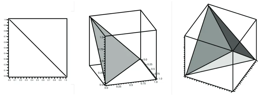
can be interpreted as a coordinate of the n-dimensional unit simplex

Multinomial distribution and the Dirichlet distribution, a fact used later. Graphical depictions

of _S2_,

S3_{, and}

S4 _{are shown in Figure 2. Note that the arithmetic mean of Equation (31) is}

not the only constraint that could be chosen. For instance, a constraint using the harmonic or geometric mean could be used instead. However, none of these alternative constraints have the justification or simplicity of interpretation of Equation (31). Also note that the rates of sites 1, 2,…,n are often considered as a sample from a larger (infinite) population, implying

that their mean need not be exactly one. We consider including such sampling variation later.

An additional benefit of the arithmetic mean constraint of Equation (31) is that the rates no longer range over the entire positive real line. Instead, the constraint 0ri n results in a

finite and bounded parameter space, implying that an infinite rate is impossible.

Objective Priors for Proportions

As we have already discussed, and as further elucidated by Kass and Wasserman, there are two related but different interpretations of what an objective prior is (1996). First is that objective priors are formal representations of ignorance. Second is that there is no objective, unique prior that represents ignorance, mainly because there is no unique notion of

ignorance. Instead, a particular objective prior should be selected for use as a default by public agreement, much like units of weight or length. We use this default when there is either insufficient information or insurmountable difficulty exists to define the prior. We define three different objective priors on the simplex support for a set of relative proportions.

The Uniform Prior

The uniform prior has been a widely used for its conceptual and mathematical simplicity. The uniform prior is identical to the maximum-entropy prior if the support of the prior is finite. Jaynes (1968) argued that if p is the density of the prior, then the entropy

H

( )

p =

plnp dμ

( )

p (32)

represents the amount of uncertainty implied by p with respect to the base density μ. For

density p that maximizes the entropy, we maximize the uncertainty and hence minimize the

information present in the prior.

Although maximum entropy priors have been used successfully in a broad range of problems, it is not necessarily ideal for all circumstances. For instance, they are not invariant to reparameterization, and they are subject to numerous inferential paradoxes. For a review and critique of maximum-entropy priors, please refer to Seidenfeld (1987).

The Multinomial Prior

Invariance to reparameterization is a highly desirable property for a prior. Unfortunately, developing such a prior satisfying Equations (24) and (25) is difficult for a likelihood given by Equation (17). Consider that the estimated quantities denote a set of relative

proportions. With the ansatz that when nothing else is known, any set of experiments that measure a set of relative proportions should have the same prior for them. Thus, all

experiments should share the same prior. Now consider the following experiment: a large set of colored balls, with n different colors, is placed in an urn. Balls are sampled with

replacement with the goal of inferring the relative proportions of colors. This experiment describes a classic inferential problem based on the multinomial distribution, and has been extensively studied. Associating the relative fraction of each color with the relative rate fraction i, we draw an analogy between the inference of multinomial parameters and rate

fraction parameters.

For inference about multinomial parameters, Jeffreys (1946; 1961) proposed using a reparameterization-invariant prior that is proportional to the square root of the determinant of the Fisher information matrix

P d

( )

detI

(

A,T

)

d , (33)

where I

(

A,T

)

denotes the Fisher information matrix of the likelihood. Applied to a set of

unknown proportions with multinomial likelihood, Jeffreys’ procedure results in the prior

P d

( )

d

12n

This so-called the Jeffreys prior works well for univariate priors. In the multivariate case it is known to sometimes give results incommensurate with conventional statistical theory

(Syversveen 1998). Therefore, the Jeffreys prior should not be accepted as the multivariate “prior of choice” without additional justification.

To ameliorate problems with the multivariate Jeffreys prior, the reference prior

construction was created by Bernardo (1974), further refined by Berger and Bernardo (1989), and fully developed Bernardo and Smith (1994). This class of priors is identical to the

Jeffreys prior in the univariate case, but is often quite advantageous to the Jeffreys prior in the multivariate case. A “reference prior” is a prior that maximizes the expected Kullback-Leibler divergence of the posterior distribution relative to the prior. This maximizes the expected posterior information about when the prior density is P d

( )

. The case of

inferring multinomial proportions has been analyzed in detail by Berger (1992) and Bernardo (1998). Their analyses yield results identical to the Jeffreys prior, a coincidence giving strong evidence for the correctness and consistency of the Jeffreys prior for the multinomial

distribution.

Goyal (2005) showed that the Jeffreys prior can also be obtained from, and is logically equivalent to, an intuitively reasonable information-theoretical invariance principle in the limit as n . This result is comforting because the greatest criticism of the ansatz equating balls in an urn with evolutionary rates is the fact that the analogy only holds if it is given that there are an infinite number of balls.

The Group-Invariant Prior

Group-invariant priors are constructed to be invariant to specific types of group

operation, rather than arbitrary reparameterization. For instance, given a three-site alignment,

the prior information we have about rates

{

r1,r2,r3

}

is identical the prior information we have

of the permuted rates

{

r3,r1,r2

}

, thus the prior for these rates should be invariant to

Another type of desirable group-invariance is based on a more subtle argument. Given

three unknown rate proportions

{

1,2,3

}

, suppose we have three known positive constants

a,b,c

{

}

. Our ignorance of

{

₁,₂,₃

}

, is equal to our ignorance of the scaled relative proportions

{

a₁,b₂,c₃

}

, after normalization. The process of scaling and normalization

defines a Lie group on _Sn_{, and this group is isomorphic to the standard Euclidian group of}

n1 _{under addition. Details, including proof of the wider result that}

Sn _{is isomorphic to the} vector space n1_{, are in Egozcue et al. (2003).}

The appropriate prior for Lie group invariance to hold is given by the Jacobian of the

transformation T :Sn n1_{, given by}

P d

( )

d

12n . (35)

It formally encapsulates the idea that if x>0 is unknown and y>0 is known, our ignorance

of x the same as our ignorance of xy. The fact that this prior is improper is an unfortunate

but not insurmountable difficulty.

Relating the Priors

The most notable connection among the priors discussed is that, despite having diverse philosophical and logical underpinnings, all three priors are members of the same distribution family. Specifically,

Dirichlet

(

,,…,

)

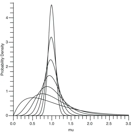
(36)

for some 0< 1, with the group-invariant prior of Equation (35) being a limiting case. It

is possible to choose >1, but we find no compelling reason to do so. A graphical

comparison of the = 0,1 2,1

{

}

cases, where n=2, is depicted in Figure 3. As decreases, increasingly more weight is given to the prior probability that is either near zero or near one, corresponding to cases of high or low conservation, respectively.

priors are frequently used in Bayesian analysis, they cannot be used here since they will always result in an improper posterior. Worse, as the prior becomes more singular, numerical methods often ill-conditioned. Therefore should not be too small.

Computing the Posterior

Given a likelihood of the form of Equation (17) and a model of amino acid replacement, the posterior rate distribution can be sampled the Metropolis-Hastings (MH) Markov Chain Monte Carlo (MCMC) technique (Robert and Casella 2004). Amino acid transition

probabilities were specified by the wag evolutionary Markov process of Whelan and

Goldman (2001) such that the probability of transition from amino acid k to amino acid j is

given by

P j k

(

,rt

)

= er t Q

j.k, (37)

where Q is the wag rate matrix. The prior probability of observing amino acid x, denoted by

P x

( )

in Equation (17), was taken as the wag default.

Sampling the Posterior

The MH-MCMC algorithm is a three-step process. Given an initial parameter estimate

old, a new estimate new is drawn from density P

(

new old

)

. The new value is then accepted

if

u< P

(

old new

)

P

(

new A,T

)

P

(

new old

)

P

(

old A,T

)

, (38)

where u is drawn from a uniform

[ ]

0,1 -distribution, and rejected otherwise. The procedure

is iterated indefinitely, resulting in consecutive parameter values being samples from the posterior.

Correct specification of the proposal density P

(

new old

)

is important. Since the Dirichlet

leads to unacceptable MCMC convergence, likely due to the highly asymmetrical nature of the Dirichlet density when its parameters are very small or very large, resulting in a low acceptance rate. We were unable to find any variation of Dirichlet-based proposal densities that had displayed acceptable convergence properties.

Instead, a variation of a simplex point-picking algorithm was used to indirectly derive a proposal density such that repeated sampling from the proposal density was equivalent to performing a uniform random walk over the simplex. Traditionally, simplex point-picking is accomplished via well-known properties connecting the Dirichlet and Gamma distributions.

Specifically, if is uniformly distributed over _Sn_{, then}

Dirichlet 1,1,

(

…,1

)

and draws of can be made by summing and normalizing n unit-exponential deviates (Devroye 1986).

For our purposes, an alternative point picking algorithm based on order statistics

(Balakrishnan and Cohen 1991), as proposed by Kraemer (1999) and refined by Smith and Tromble (2004), is more constructive. They recommend the following steps to generate :

Set x0 0 and xn 1.

Generate n1 uniform random values from the open interval xi

( )

0,1 .

Sort the set of points

{

x₀,x₁,…,x_n

}

into increasing order.

The n final coordinates

{

₁,₂,…,n

}

are given by i xi xi1.

If any i =0, rerun the algorithm to generate a new set of .

Viewing the n1 internal coordinates xi as particles within a unit-interval “box” yields an

immediate procedure for perturbing in a manner guaranteed to uniformly sample the simplex. Given an initial n1 points xi, as above, and a maximum displacement

0<max 1, iterate the following:

1. Draw a set of random

{

₁,₂,…,_n1

}

, such that _max<i max uniformly.