ABSTRACT
WANG, JIANGDIAN. Shape Restricted Nonparametric Regression with Bernstein Polynomials. (Under the direction of Sujit K. Ghosh.)
There has been increasing interest in estimating a multivariate regression function subject
to various shape restrictions, such as nonnegativity, isotonicity, convexity and concavity among
many others. The estimation of such shape-restricted regression curves is more challenging for
multivariate predictors, especially for functions with compact support. Most of the currently
available statistical estimation methods for shape restricted regression functions are generally
computationally very intensive. Some of the existing methods have perceptible boundary biases.
This thesis considers a suitable class of univariate and multivariate Bernstein polynomials
and proposes sieved estimators obtained from a nested sequence of shape-restricted
multivari-ate Bernstein polynomials. The proposed nonparametric estimators are shown to be: (i) the
regression function estimate is shown to be the solution of a quadratic programming problem;
making it computationally attractive (ii) the nonparametric estimator is shown to be
univer-sally consistent under some mild regularity conditions and (iii) the estimation methodology is
flexible in the sense that it can be easily adapted to accommodate many popular multivariate
shape restrictions. Numerical results derived from simulated data sets and real data analysis
are used to illustrate the superior performance of the proposed estimators compared to a few
other existing estimators in terms of various goodness of fit metrics.
The inference is derived through the bootstrap method and the bayesian method, as the
standard methods to derive asymptotic distributions may not be applicable directly to the
esti-mator. In addition, we extend our ordinary estimator obtained from shape-restricted Bernstein
polynomials and apply it in the linear mixed effects model framework. The work is motivated
by a longitudinal data, and the proposed estimator is obtained through iterative methods. We
show the effectiveness of our algorithm through both simulations and the real data study.
modifying the ordinary algorithm to an iterative estimation method. The proposed estimator
c
Copyright 2011 by Jiangdian Wang
Shape Restricted Nonparametric Regression with Bernstein Polynomials
by Jiangdian Wang
A dissertation submitted to the Graduate Faculty of North Carolina State University
in partial fulfillment of the requirements for the Degree of
Doctor of Philosophy
Statistics
Raleigh, North Carolina
2012
APPROVED BY:
Barry Goodwin Huixia (Judy) Wang
Brian Reich Sujit K. Ghosh
DEDICATION
To my father, my husband
BIOGRAPHY
Jiangdian Wang was born on February 23rd, 1981 in Fuzhou, China. She got her Bachelor of
Science degree in Electronic and Computer Engineering from Zhejiang University, Hangzhou,
China in July 2003. After that, she worked as a research assistant in Singapore. To seek a
graduate education, she came to the United States. She got her Master degree in Statistics at
North Carolina State University (NCSU) in August 2009 and she has been to pursue a Ph.D.
degree in Statistics since then. Her research focuses on the methodology of nonparametric
ACKNOWLEDGEMENTS
I would like to express my deep and sincere appreciation to my advisor Professor Sujit K.
Ghosh for his patience, motivation, enthusiasm, and immense knowledge. His great guidance,
encouragement and support helped me in all the time of research and writing of this thesis. I
could not have imagined having a better advisor and mentor for my Ph.D study.
Besides my advisor, I would like to thank my committee members: Professor Judy Wang,
Professor Brian Reich, and Professor Barry Goodwin for their valuable helps and insight
com-ments.
My appreciations also go to Dr. Pam Arroway, Professor Leonard Stefanski, Professor John
Monahan and Professor Sujit K. Ghosh. They are brilliant Directors of Graduate Programs
(GDPs). Dr. Arroway and Professor Stefanski approved my application to transfer from the
department of ECE, and offered me the Teaching Assistant scholarship. Without their helps,
I would still be a suffering student there. Dr. Arroway gave me incredible encouragements
and supports when she was in our department. Professor Monahan and Professor Ghosh are
our current GDPs. They work very hard to provide more and more opportunities to students
(including me), encourage us to attend several academic conferences, and solve my financial
support issue.
I am lucky to receive the support and encouragement from all my friends in the department.
We have had many great moments together and I would like to thank them for sharing the happy
school life with me in the last few years.
Last but not the least I would like to thank my parents and my husband for all their endless
love and support. They always have confidence in me and always encourage me to overcome
TABLE OF CONTENTS
List of Tables . . . .viii
List of Figures . . . x
Chapter 1 Introduction to Shape Restricted Regression . . . 1
1.1 Shape Restricted Regression with a Single Predictor Variable . . . 2
1.2 Shape Restricted Regression with Multiple Predictor Variables . . . 6
1.3 Bayesian Models for Shape-Restricted Regression . . . 8
1.4 Bernstein Polynomials . . . 9
1.4.1 Univariate Bernstein Polynomials . . . 9
1.4.2 Multivariate Bernstein Polynomials . . . 13
1.5 Organization of The Thesis . . . 14
Chapter 2 Shape Restricted Nonparametric Regression with Univariate Bern-stein Polynomials . . . 15
2.1 Introduction . . . 15
2.2 Restricted Bernstein Polynomial Estimator . . . 19
2.2.1 Examples of Constraint Bernstein Polynomial Sieves . . . 21
2.2.2 Computation of the Sieved Estimator . . . 23
2.3 Asymptotic Properties . . . 25
2.4 Simulation Studies . . . 29
2.4.1 Monotone Regression . . . 29
2.4.2 Increase-concave Regression . . . 32
2.5 Real Data Examples . . . 34
2.5.1 Fuel Efficiency Study using ASA Car Data . . . 34
2.5.2 Growth Curve Study using Rabbit Data . . . 35
2.6 Conclusion . . . 36
Chapter 3 Shape Restricted Nonparametric Regression with Multivariate Bern-stein Polynomials . . . 43
3.1 Introduction . . . 43
3.2 Modelling Shape Restrictions Using Multivariate Bernstein Polynomials . . . 47
3.2.1 Constraint Bernstein Polynomial Sieve (d= 2) . . . 49
3.2.2 Computational Details . . . 54
3.3 Asymptotic Properties . . . 56
3.4 Simulation Studies . . . 60
3.4.1 Data Generation and Computational Details . . . 61
3.4.2 Results . . . 62
3.5 Real Data Application . . . 66
Chapter 4 Inference using Bootstrap and Bayesian Methods . . . 84
4.1 Introduction . . . 84
4.2 Bootstrap Method . . . 85
4.2.1 Bootstrap Distribution of Estimator ˆmN(x) . . . 86
4.2.2 Real Data Example . . . 87
4.3 Bayesian Method . . . 89
4.3.1 Bayesian Approach to Shape Restricted Regression . . . 90
4.3.2 Simulation Studies . . . 97
4.3.3 Real Data Application . . . 103
4.4 Conclusion . . . 104
Chapter 5 Mixed Effects Model Subject to Shape Restrictions . . . .109
5.1 Introduction . . . 109
5.2 Models and Algorithms . . . 111
5.2.1 Linear Mixed Models . . . 114
5.2.2 Iterative Method for Linear Mixed Model with Heteroscedastic Errors . . 115
5.2.3 Extension to Shape Restricted Mixed Regression Model . . . 118
5.3 A Simulation Study . . . 120
5.4 Real Data Application . . . 121
5.5 Discussion . . . 126
Chapter 6 Shape Restricted Nonparametric Regression with Heteroscedastic Errors . . . .130
6.1 Introduction . . . 130
6.2 Models and Algorithms . . . 132
6.2.1 Estimator . . . 133
6.2.2 Computation of the Estimator . . . 134
6.3 Simulations . . . 137
6.4 Infant Mortality Rate Data Example . . . 139
6.5 Conclusion . . . 140
Chapter 7 Discussions and Future Work . . . .143
7.1 Bayesian Model with Varying Dimensions . . . 144
7.2 Testing for Shape Restrictions . . . 145
References. . . .147
Appendices . . . .153
Appendix A Detailed Proofs of Asymptotic Properties . . . 154
A.1 Proof of Property 3.3.1 . . . 154
A.2 Proof of Property 3.3.2 . . . 157
A.3 Proof of Lemma 3.3.1 . . . 158
A.4 Proof of Lemma 3.3.2 . . . 159
LIST OF TABLES
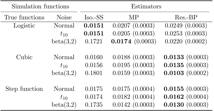
Table 2.1 Average integrated mean squared errors (IMSE) over 1000 repetitions. The sample size isn= 50 and all the noise distributions are centered and scaled to have mean zero and standard deviation σ= 0.4. Standard error of IMSE is displayed in the parentheses. . . 37 Table 2.2 Average integrated mean squared prediction errors (IMSPE) over 1000
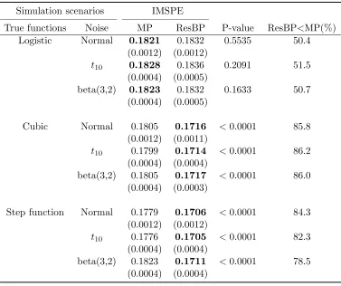
repetitions. The sample size is n = 50 and all the noise distributions are centered and scaled to have mean zero standard deviation σ = 0.4. Standard error of IMSPE is displayed in the parentheses. P-values are obtained based on two-sample t-tests. . . 38 Table 2.3 Average integrated mean squared errors (IMSE) over 1000 repetitions. The
sample size is n = 50 and the noise has standard deviation σ = 0.5 and 0.1. Standard error of IMSE is displayed in the parentheses. P-values are obtained by using two-sample t-tests between the BP method and the rest methods. . . 38
Table 3.1 RMISE and MIAE (×100) for m1(x1, x2) = min(x1, x2) based on 500 Monte Carlo replications as global measurements of performance. Note: Standard error is displayed in the parentheses. BP stands for the proposed Bernstein polynomial based estimate. MP stands for the monoProc estimate. 71 Table 3.2 RMISE and MIAE (×100) for m2(x1, x2) = x1x2I(x1 ≤ 0.5, x2 ≤ 0.5) +
{(x1−0.5)(x2−0.5)+x1x2}I(x1 >0.5, x2 >0.5) based on 500 Monte Carlo replications as global measurements of performance. Note: Standard error is displayed in the parentheses. BP stands for the proposed Bernstein polynomial based estimate. MP stands for the monoProc estimate. . . 71
Table 3.3 RMISE and MIAE (×100) for m3(x1, x2) = x13
1x
2 3
2 based on 500 Monte
Carlo replications as global measurements of performance. Note: Standard error is displayed in the parentheses. BP stands for the proposed Bernstein polynomial based estimate. MP stands for the monoProc estimate. . . 72 Table 3.4 Prediction biases for m1(x1, x2) = min(x1, x2) based on 500 Monte Carlo
replications as local measurement of performance. Column 3 and 4: Mean bias (S.E. of bias); Column 5 and 6: [2.5th percentile, 97.5th percentile] of the biases. . . 72 Table 3.5 Prediction biases for m2(x1, x2) = x1x2I(x1 ≤ 0.5, x2 ≤ 0.5) +{(x1 −
Table 3.6 Prediction biases for m3(x1, x2) = x11/3x22/3 based on 500 Monte Carlo replications as local measurement of performance. Column 3 and 4: Mean bias (S.E. of bias); Column 5 and 6: [2.5th percentile, 97.5th percentile] of the biases. . . 73 Table 3.7 Pearson correlations with Kendall’s Tau in parenthesis among three variables. 73
Table 4.1 Simulation study for m1(x) = sin(π2x). The results are averaged over 200 Monte Carlo replications. Monte Carlo standard error is displayed in the parentheses. . . 102 Table 4.2 Simulation study form2(x) = 2x·I(x∈[0,0.25])+ 0.5·I(x ∈[0.25,0.75])+
(2x−1)·I(x∈[0.75,1]). The results are averaged over 200 Monte Carlo replications. Monte Carlo standard error is displayed in the parentheses. . 102 Table 4.3 Simulation study for m3(x) = (16/9)(x−1/4)2. The results are averaged
over 200 Monte Carlo replications. Monte Carlo standard error is displayed in the parentheses. . . 103 Table 4.4 Simulation study for m4(x) = (−4x + 1)·I(x ∈ [0,0.25]) + 0 ·I(x ∈
[0.25,0.75]) + (4x−3)·I(x∈[0.75,1]). The results are averaged over 200 Monte Carlo replications. Monte Carlo standard error is displayed in the parentheses. . . 103
Table 5.1 Summary of ˆβestimations. The results are based on 100 MC repetitions. . 121
LIST OF FIGURES
Figure 2.1 An increasing-concave curve (solid), and observed data (scatter plot). . . 39 Figure 2.2 Box plots of predicted responses. The sample size isn= 50 and the noise
has standard deviation σ = 0.5. . . 40 Figure 2.3 ASA car fuel efficiency as a function of engine output. Top left: Convex
and decreasing BP estimator (with ˆN = 12). Top middle: Convex BP estimator (with ˆN = 17). Top right: Decreasing BP estimator (with
ˆ
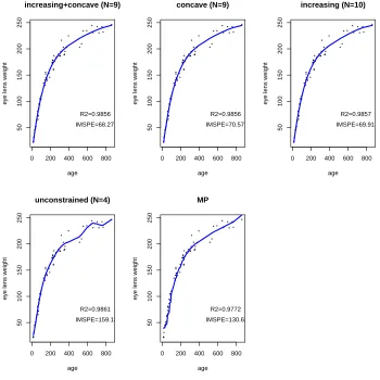
N = 17). Bottom left: Unconstrained BP estimator (with ˆN = 7). Bottom middle: MP decreasing estimator. . . 41 Figure 2.4 Eye lens weight for rabbits as a function of age. Top left: Concave and
increasing BP estimator (with ˆN = 9). Top middle: Concave BP estima-tor (with ˆN = 9). Top right: Increasing BP estimator (with ˆN = 10). Bottom left: Unconstrained BP estimator (with ˆN = 4). Bottom middle: MP increasing estimator. . . 42
Figure 3.1 3-D plots of two shape-restricted regression functions: (a)f(x1, x2) = x21+ 2e−x22+14x1(x2+ 2) (left panel); (b)f(x1, x2) =x11/3x22/3 (right panel). 74 Figure 3.2 3-D surface plots and contour plots for m1(x1, x2) = min(x1, x2) when
σ2 = 0.01 and n = 400. Note: Data is randomly generated from one Monto Carlo simulation out of 500 simulations. From top to bottom: surface plots, and contour plots. From left to right: true curve, monoProc (MP) method, and restricted Bernstein Polynomial (BP) method. . . 75 Figure 3.3 3-D surface plots and contour plots form2(x1, x2) =x1x2I(x1 ≤0.5, x2≤
0.5) +{(x1−0.5)(x2 −0.5) +x1x2}I(x1 >0.5, x2 >0.5) whenσ2 = 0.01 and n= 400. Note: Data is randomly generated from one Monto Carlo simulation out of 500 simulations. From top to bottom: surface plots, and contour plots. From left to right: true curve, monoProc (MP) method, and restricted Bernstein Polynomial (BP) method. . . 75
Figure 3.4 3-D surface plots and contour plots form3(x1, x2) =x13
1x
2 3
2 whenσ2 = 0.1
and n= 400. Note: Data is randomly generated from one Monto Carlo simulation out of 500 simulations. From top to bottom: surface plots, and contour plots. From left to right: true curve, monoProc (MP) method, and restricted Bernstein Polynomial (BP) method. . . 76 Figure 3.5 Plot of average predicted values vs. true values form1(x1, x2) = min(x1, x2).
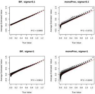
Solid line is 45◦ reference line. . . 76 Figure 3.6 Plot of average predicted values vs. true values form2(x1, x2) =x1x2I(x1 ≤
0.5, x2 ≤0.5) +{(x1−0.5)(x2−0.5) +x1x2}I(x1 >0.5, x2 >0.5). Solid line is 45◦ reference line. . . 77 Figure 3.7 Plot of average predicted values vs. true values for m3(x1, x2) = x
1 3
1x
2 3
2.
Figure 3.8 Box plots of bias at five points using the BP and the MP method with sample size n=400 and 500 replications. Note: Simulation scenarios are described as follows. From top to bottom: σ = 0.1 and σ = 1.0; From left to right: m1(x1, x2) = min(x1, x2),m2(x1, x2) =x1x2I(x1 ≤0.5, x2≤ 0.5) +{(x1−0.5)(x2−0.5) +x1x2}I(x1 >0.5, x2 >0.5), andm3(x1, x2) = x113x223. . . 79 Figure 3.9 Optional caption for list of figures . . . 80 Figure 3.10 Predicted values of ˆm(x1i, x2i) vs. predictors x1i and x2i. i=1,...,176.
Note: X1=ALT, X2=HEPC, Y=IMR. Top Panel: observed yi vs. x1i andx2i; Middle Panel: predicted values obtained by Bernstein polynomial method vs. predictors; Bottom: predicted values obtained by monoProc vs. predictors. . . 81 Figure 3.11 Comparison of observed and predicted values of the response. Solid line
represents the 45◦ reference line, i.e., y=x. . . 82 Figure 3.12 Residual vs. predicted values. Residual = predicted value - observed
re-sponse. Top panel: Bernstein polynomial based estimate. Bottom panel: monoProc estimate. . . 82 Figure 3.13 Comparison of observed responses and predicted values: Reduced model
in (a), Full model in (b), and predicted values from Full model vs. Re-duced model in (c). Solid line represents the 45◦ reference line, i.e., y=x. 83 Figure 3.14 CV score vs. N for the infant mortality data. . . 83
Figure 4.1 Histogram of the Bootstrap Distribution of 10000 Resampled IMSPE’s. . 106 Figure 4.2 Simulation results over 200 simulation data sets under σ = 0.1. Scatter
plot: randomly generated data from one Monte Carlo simulation out of 200 simulations. Solid line: true regression curve. Dashed line: (average) Bayesian regression posterior median curve. Shaded region: (average) 95 percent pointwise credible (confidence) region for the Bayesian fit. Top Panel: increasing functions m1(x) = sin(π2x); m2(x) = 2x·I(x ∈ [0,0.25])+0.5·I(x ∈[0.25,0.75])+(2x−1)·I(x ∈[0.75,1]). Bottom Panel: convex functions m3(x) = (16/9)(x−1/4)2; m4(x) = (−4x+ 1)·I(x ∈ [0,0.25]) + 0·I(x∈[0.25,0.75]) + (4x−3)·I(x∈[0.75,1]). . . 107 Figure 4.3 The Rabbit data alongside the Bayesian increasing Bernstein polynomial
regression posterior mean curve (solid line) and 95 percent credible inter-vals (dotted line). . . 108
Figure 5.1 Spaghetti plot: each line represents the growth of an individual Sitka spruce tree over time. Left: control group. Right: ozone-enriched group. . 127 Figure 5.2 Box plots of βestimation. Reference lines in red represent true β’s. . . . 127 Figure 5.3 5-fold CV at the subject level . . . 128 Figure 5.4 CV score vs. N for Sitka spruce data. . . 128 Figure 5.5 Thin-plate spline fit by Crainiceanu et al. (2005) for the function for Sitka
Figure 5.6 Restricted Bernstein polynomial fit for Sitka spruces date: (a) mean growth rate fit by restricted Bernstein polynomial model; (b) ozone effect shown as growth rate difference at different time points. The fixed ozone effect obtained from Crainiceanu et al. (2005) is shown as dashed line. . . 129
Figure 6.1 The heteroscedastic estimation: the estimated regression function (black dashed), the true function (red solid), 95% confidence interval (gray). . . 141 Figure 6.2 The homoscedastic estimation: the estimated regression function (black
dashed), the true function (red solid), 95% confidence interval (gray dashed).141 Figure 6.3 The estimation of conditional variance function (dashed) vs. the true
conditional variance function (solid). . . 142 Figure 6.4 Infant mortality data (a) Raw data and the estimated regression function;
(b) Residuals and their estimated volatility function. . . 142
Chapter 1
Introduction to Shape Restricted
Regression
The statistical regression method is often used to explore the inherent relationship between
several predictor variables (usually denoted withX1, X2, ..., Xd) and a response variable (usually denoted withY). More specifically, the response variable is often assumed to have a relationship
with predictor variables as follows:
Yi =m(x1i, x2i, ..., xdi) +εi, i= 1,2, ..., n,
whereεi’s are independently distributed withE(εi|Xi) = 0 andm(x) =E(Y|X=x) whenX= (X1, ..., Xd) and x= (x1, ..., xd) denote the predictor vector and its realized value respectively. This model is called the general regression model, andm(·) is known as the regression function. In many practical settings, the predictors and the response are known to preserve certain
shape restrictions, such as monotonicity, concavity etc. For example, utility functions, cost
functions and profit functions in economics are all known to be convex or concave curves
(Gal-lant and Golub 1984; Terrell 1996). The dose response curve in the phase I clinical trial takes
failure rate in reliability and survival analysis is another typical curve with convexity
restric-tions (Chang et al. 2007; Molitor and Sun 2002). Over the past decades, efforts have been
devoted to search for a smooth and computationally efficient estimator of a shape restricted
regression function.
In this thesis, we develop a new nonparametric regression methodology which is based on
multivariate Bernstein Polynomials as basis functions. Our proposed method can be easily
adopted to fit several shape-restricted regression curves. In the remainder of this chapter,
we briefly review the relevant background literature for the estimators which are then fully
developed in the remaining chapters of this thesis. We begin by reviewing the existing methods
in the literature to estimate shape restricted regression function of a single univariate predictor.
We then review the literature on multivariate shape restricted estimators. For completeness,
we also provide a brief review of Bernstein Polynomials that are used to develop our proposed
estimator, as well as some of their fundamental properties. Finally, we end this chapter with a
discussion of the organization of this thesis proposal.
1.1
Shape Restricted Regression with a Single Predictor
Vari-able
In this section we review the literature on shape restricted regression with a single predictor
variable. Hildreth (1954) pioneered the research by proposing a maximum likelihood method
to estimate a regression function under the restrictions of concavity. The regression model
considered by Hildreth is Yij =m(xi) +εij, i = 1, ..., n,and j = 1, ..., Ji, wherexi’s represent
distinct values of predictor variable X, and Yij’s represent the replicates of observed responses
corresponding to xi. The method is based on estimating a step function subject to restrictions
range of observedxi’s. Barlow et al. (1972) proposed the Pool Adjacent Violators Algorithm
(PAVA) for solving monotonic regression problems, which is a special (univariate) case of the
problem considered by Brunk (1955). Assume the regression modelYi =m(xi) +εi, the PAVA
iteratively finds ˆmiwhich minimizesni=1(yi−miˆ ) subject to a monotonicity constraint ˆmi+1≥ ˆ
mi fori= 1,2, ..., n−1. The major shortcoming of this method is that the estimator obtained by the PAVA is not necessarily smooth (Friedman and Tibshirani 1984). A variety of the
smoothed PAVA were developed subsequently by Friedman and Tibshirani (1984) and Mukerjee
(1988) to obtain smoothed monotonic estimators. Friedman and Tibshirani (1984) combined a
running mean smoother with the PAVA algorithm. They first smoothed the data by taking the
average of the current prediction values with a certain number of the nearest neighbors and
then monotonizing the fit using PAVA. Mukerjee (1988) on the other hand obtained the isotonic
estimator by the PAVA algorithm first, and then smoothed the fit using a kernel smoother.
Ramsay (1988) pioneered the use of regression splines for monotone regression functions.
The method is based on utilizing the I-spline basis (the integrated M-spline basis) for monotone
splines. Assume that the regression function is defined in an interval [L, U] which is subdivided
at the points L=ξ1<· · ·< ξq=U. Let {t1,· · · , tn+k} be a set of designated positions along thex-axis (or knots) by replacing boundary valueξisuch thatt1≤ · · · ≤tn+k,t1=...=tk=L, tn+1 = ... = tn+k = U, tk+i = ξi and ti < ti+k for all i. M-spline functions of order k with n free parameters are piece-wise polynomials of degree k−1 defined at the knot sequence t. The I-spline basis is the integration of M-spline, and known as a piecewise polynomial of degree
k. The monotone regression function is estimated using a linear combination of I-spline basis
functions. The isotonic regression estimator by Barlow et al. (1972) is a special case of the
I-spline method when k = 1. More recently, Meyer (2008) extended the method in Ramsay
(1988) and proposed convex C-splines (integration of I-splines) to fit spline regression with
convex constraints.
He and Shi (1998) presented another smoothing spline method using B-spline as basis
subject to π(xi)Tα ≥ 0 for i = 1, ..., n. π(x) = (π1(x), π2(x), ..., πN(x))T denotes normalized B-splines of degree two (quadratic spline), π denotes the derivative of π, and α is a vector
of spline coefficients. The restriction π(xi)Tα ≥ 0 ensures the monotonicity of the resulting spline fit. The optimization can be solved using quadratic programming method. In addition,
the number of knots k is determined by a criterion similar to Akaike information criterion
(AIC). Similarly, Wang and Li (2008) presented an estimator for monotone smoothing spline
regression. The regression function is constructed to build upon the natural cubic splines.
Another type of method for regression subject to monotonicity constraints is kernel-type
estimators (Hall and Huang 2001; Dette et al. 2006). Hall and Huang (2001) suggested a
method to monotonize a general kernel-type estimator of a regression function (e.g.
Gasser-M¨uller, Nadaraya-Watson, Priestley-Chao, local linear estimators, etc.). They generalized the
definition of the linear estimator to be a weighted sum of observed responses expressed as
ˆ
m(x) = ni=1piAi(x)yi, where p = (p1, ..., pn) is a set of probability weights supported on the observed x-values {x1, ..., xn}, and the weight functions Ai depends on a specific kernel function. The proposed monotone kernel regression estimator is obtained by choosing a proper
value of p which minimizes a well-defined distance D(p) from p to the uniform distribution p0 = (1/n, ...1/n). Dette et al. (2006) combined an unrestricted regression estimate with a den-sity estimate to produce the new monotone estimator. As proposed, the inverse of the monotone
estimator is given by ˆm−1(t) = nh1
d
n i=1
t
−∞Kd(φ(i/nhd)−u)dt, whereφ(x) =
n
i=1Kr((Xi−x)/hr)Yi
n
i=1Kr((Xi−x)/hr)
is the classical Nadaraya-Watson estimate, Kd andKrare proper symmetric kernels with finite
second moments, andhd,hr are corresponding bandwidths for regression estimate and density
estimate. The accuracy of the regression results greatly relies on the proper choice of tuning
parameters hd and hr. Although this method does not require constrained optimization, the
selection of tuning parameters can be problematic and make an impediment in the practical
implementation. Birke and Dette (2007) extended the method in Dette et al. (2006) to fit a
convex regression.
projection of the data with respect to proper norms, and took one step further to propose a
new projection based estimator. Assume a vector space denoted by Vs containing all possible candidate regression functions space denoted by Vsm and a space of data vectors VsY. The space of all possible constrained smooth function is denoted by Csm, and obviously Csm ⊂ Vsm. Then unconstrained estimator ˆmsminimizes the objective function||−→−Y −→||m 2 in theVsmspace. Similarly, the constrained estimator ˆms,c minimizes ||−→ −Y →||−m 2 in the Csm space. Here, −→Y is a vector of constant functions with fi(x) = Yi, and −→m is a vector of the same function with fi(x) = m(x) for all i. Using a Pythagorean relationship, ||−→ −Y −→||m 2 yields to be the sum of ||−→ −Y −→ms||2 and ||−→ms −→||−m 2, where ˆ−→ms is the projection of −→Y on the space Vsm. Using this decomposition, the constrained estimator turned out to be the projection of the
unconstrained estimator on the spaceCsm. Therefore, Mammen et al. (2001) suggested deriving an unconstrained smooth estimator first, and finding the projection of the fit on the constrained
space.
Birke and Dette (2007) pointed out that the least squares based as well as the projection
based estimators are not smooth enough, in the case that the underlying regression function
is known to be smooth. In addition, some of these estimators suffer from the computational
inefficiency. For example, the least squares based convex estimators in Dykstra (1983) and Han
(1988) are usually calculated by the procedure of iterative loops. Moreover, a few methods
are believed to be too complicated to handle the large sample case (e.g., sample size n >
10,000). For example, the estimator in A¨ıt-Sahalia and Duarte (2003) requires one to construct
restrictions at each individual observed data point, and thus number of constraint conditions
could be as large as the sample size. Another drawback is that many of these estimators
guarantee to maintain the convexity and/or other shape constraints only at observed data (i.e.,
atxi’s only). Hence such shape constraint might be violated at prediction points which are not
in the vicinity of the observed data. The monotone estimator by Hildreth (1954) is a typical
1.2
Shape Restricted Regression with Multiple Predictor
Vari-ables
The literature for shape restricted regression problems with more than one predictor is relatively
scarce. The study begins with Brunk (1955). Brunk used the similar maximum likelihood
method in Hildreth (1954) and derived an estimator for monotone parameters in the exponential
family of distributions. This method has the same drawback as the one of Hildreth (1954), that
the estimator can only provides estimation for the values of predictors observed in the data set.
In order to interpret the individual effects of each predictor variable easily, Bacchetti (1989)
presented an additive isotonic regression model which also has the link function to allow its
use in generalized linear models. Bacchetti borrowed the standard PAV algorithm by Barlow
et al. (1972) as well as some other algorithms, and defined the cyclic pooled-adjacent-violators
algorithm for fitting additive isotonic regression models. The proposed estimator inherits some
drawbacks of the PAVA algorithm. For instance, the resulting estimator is not necessary smooth
and exhibit the step function like behavior when the observed data seem to be partitioned into
groups.
Villalobos and Wahba (1987) presented a smoothing spline estimator using
inequality-constrained thin-plate splines. Their proposed estimator minimized the objective function
which is defined as the sum of a L2 norm and the thin-plate penalty function. The tuning parameter which controls the smoothing level is chosen using the generalized cross-validation.
The shape constrains are enforced on a fine regular grid in a subset of Euclidean space Rd.
Therefore, it may fail to preserve the desired shape restrictions outside this grid. The approach
was applied to estimate a bivariate distribution which is strictly concave in one dimension and
monotone in the other dimension, and the resulting fit failed to satisfy the concavity in some
areas. Mammen et al. (2001) pointed out that the fitted spline smoother by Villalobos and
Wahba (1987) does not guarantee to satisfy the shape constraints everywhere on the support of
in-clude Beresteanu (2004), Bollaerts, Eilers and van Mechelen (2006), and Leitenstorfer and Tutz
(2007). Beresteanu (2004) constructed a sieve least squares estimator. The basis function used
is the familiar normalized B-splines. Beresteanu restricted the coefficients of B-splines basis
to satisfy shape restrictions. The method can be solved using quadratic programming
tech-nique. Bollaerts, Eilers and van Mechelen (2006) presented P-splines regression with additional
asymmetric discrete penalties to fit a multivariate isotonic regression curve. Leitenstorfer and
Tutz (2007) also introduced a B-spline based estimators under monotonicity constraints. These
three methods all assume that the observed values of the predictor variables lie on equidistant
grids of predictor domain. If the sample size is relatively small, then having a small and discrete
number of knots can only allow very limited control over smoothness and flexibility. The fit is
especially problematic in higher dimensions.
To allow for the presence of more relaxed spatial arrangement of observed predictors
val-ues, Dette and Scheder (2007) presented a kernel-based approach to estimate multivariate
non-parametric regression function which is strictly monotone in all or a subset of its arguments
and established rigorous asymptotic results of their proposed estimator. The method in Dette
and Scheder (2007) is a natural extension of the univariate monotone estimator in Dette et al.
(2006) to two or more variables. Therefore, the method cannot escape some of the drawbacks of
the univariate version like the choice of the tuning parameters. In addition, this method could
be considerably time consuming to implement even with only moderately large sample size
(e.g., with two predictors and a sample size of only 400, it takes on average around 286 seconds.
For the same scenario, our proposed method takes only 6.36 seconds on average). Moreover,
their method is limited to fit only monotonic curves and it is not clear how the method can be
1.3
Bayesian Models for Shape-Restricted Regression
Bayesian methods for a regression problem begins with the joint distribution p(θ,Dn) of the parameters θand the observed data Dn. Following the Bayes’ theorem, we have
p(θ|Dn)∝p(Dn|θ)p(θ),
where p(θ|Dn) denotes the posterior distribution of θ (i.e., the distribution of parameters θ obtained by combining the information from the data with the information from the prior
dis-tribution),p(θ) denotes the prior distribution ofθ, andp(Dn|θ) denotes the likelihood function. Lavine and Mockus (1995) first applied a nonparametric Bayesian approach to estimate
an isotonic regression function. The method used the Dirichlet process by assigning a prior
distribution on a space of distribution functions which are nondecreasing. The most notable
drawback of using a Dirichlet process is that the probability measures are almost discrete.
Therefore, if the true regression function is smooth, the Dirichelet process is not a proper prior
distribution. Holmes and Heard (2003) proposed another Bayesian piecewise-constant model
for a monotonic regression function. In their approach, they considered a random number of
constant pieces and random locations of these knots, and then gave a prior distribution. The
approach itself does not add any constraint onto the prior distribution. The monotonicity
con-straint was guaranteed by discarding all posterior samples that does not satisfy the concon-straint.
The idea is straightforward to implement, but could be very inefficient.
The approach by Neelon and Dunson (2004) adopted a piecewise-linear model for a unknown
monotone regression function. To assign the prior distribution ofβ, the coefficients in the
piece-wise linear model, Neelon and Dunson (2004) chose a density consisting of the mixture of point
masses and truncated normal densities. Then the MCMC algorithm was used to obtain the
posterior distributions and the estimation of the regression function. However, it is believed
that the piecewise linear function may not be appropriate to model the unknown regression
al. (2007) used Bernstein polynomial expansions as basis function to fit nonparametric
shape-restricted regression functions. They considered monotonic, unimodal and unimodal-concave
as shape constraints. Bayesian algorithm was applied by placing prior distributions on the
co-efficients of Bernstein polynomial expansions. The authors claimed that the prior distributions
of model parameters satisfy certain shape-constraints, but the detailed prior distributions were
not explicitly given in the literature. The authors used reverse jump MCMC as the sampling
scheme from the posterior distribution, but the algorithm was not clearly expressed either in
the article.
1.4
Bernstein Polynomials
The Bernstein polynomial is one of the most popular class of polynomials in approximation
theory. It was introduced by S.N. Berstein in 1912 which he used to provide a constructive
proof to the famous Weierstrass approximation theorem. In this section, we briefly review
both univariate and multivariate Bernstein polynomials, followed by introducing some of their
fundamental properties available in the literature of approximation thoery.
1.4.1 Univariate Bernstein Polynomials
Let f : [0,1]→Rbe a continuous function. The Bernstein polynomial of the degree N of f(·) on the interval [0,1] is defined by (Lorentz 1986),
BN(f)(x) = N k=0 f k N
·bk(x, n) = N k=0 f k N · N k
xk(1−x)N−k.
Note that, if f is defined on the closed interval [a, b], then the corresponding Bernstein
poly-nomial is written as BN(f; [a, b])(x) = (b−1a)N
N
k=0f(a+k b−a
N )· N
k
(x−a)k(b−x)N−k. It has been shown that as the orderN grows, the Bernstein polynomial of a continuous function
converges to the function uniformly (see Bernstein (1912) or Lorentz (1986) for more details).
That is, lim
assume f : [0,1]→Ris a continuous function throughout.
The Bernstein polynomial is appropriate for shape-preserving regression, as it has the
opti-mal shape restriction property among all polynomials (Carnicer and Pena 1993). Here we list
a few shape-preserving properties of the Bernstein polynomial. The complete proofs of these
properties and many other interesting properties can be found in Chapter 1 of the excellent
book by Gal (2008).
• Iff is convex (strictly convex) of orderk∈ {0,1,2, ..., N} on [0,1], then BN(f) is convex (strictly convex) of order k on [0,1], for all N ∈ N; here notice that the usual convex function is of orderk= 1.
• If f is quasi-convex of order k ∈ {0,1,2, ..., N} on [0,1], then BN(f) is quasi-convex of order k on [0,1], for all N ∈ N; here notice that a real-valued function f : [a, b] → R defined on [a, b] of a real vector space is quasi convex if whenever x1, x2 ∈ [a, b] and λ∈[0,1] then f(λx1+ (1−λ)x2)≤max(f(x1), f(x2)).
• If f is u-monotone, where u(x) = xλ, for all x ∈ [0,1] and λ ∈ (0,1) is arbitrary and fixed, thenBN(f) is u-monotone for alln∈N. Here notice that a function f ∈C[a, b] is u-monotone if ∃u ∈C[a, b], u(x) >0, and u(x1)f(x2)−u(x2)f(x1) ≥0 for all a≤x1 < x2 ≤b.
A (univariate) Bernstein polynomial of order (or degree)N is defined as a linear combination
of Bernstein basis polynomials (Lorentz 1986),
BN(x;β) = N
k=0
βk·bk(x, N) whereβ = (β0, ..., βN),
where βk are Bernstein coefficients, and bk(x, N) are Bernstein basis polynomials. TheN + 1
Bernstein basis polynomials of orderN are defined as
bk(x, N) =
N k
xk(1−x)N−k,
N k
= N!
where k= 0,1, ..., N and 0≤x≤1. From the definition, it is easy to show that all Bernstein basis polynomials are non-negative for allx∈[0,1]. The Bernstein basis polynomials have the following nice properties (Lorentz 1986; Joy 2000).
• The Bernstein basis polynomials of orderN can be recursively represented by the sum of two Bernstein polynomials of orderN−1. More precisely,
bk(x, N) = (1−x)·bk(x, N −1) +x·bk−1(x, N−1).
Using this fact, we obtain the following property,
N
k=0
bk(x, N) = N−1
k=0
bk(x, N −1) =...=
1
k=0
bk(x,1) = (1−x) +x= 1.
• Bernstein basis polynomials of order N −1 can be expressed as a linear combination of Bernstein basis polynomial of order N. That is,
bk(x, N−1) = N−k
N bk(x, N) + k+ 1
N bk+1(x, N).
It is easy to show that any Bernstein basis polynomial with the order less thanN can be
written as a linear combination of Bernstein basis polynomials of orderN.
• The derivatives of Bernstein basis polynomials are polynomials of lower order. That is,
bk(x, N) = d
dxbk(x, N) =N ·[bk−1(x, N−1)−bk(x, N−1)].
extended to higher order derivatives. More precisely,
BN(l)(x, β) = N! (N−l)!
N−l
k=0
∇(l)β
kbk(x, N −l) =BN−l
x, N! (N −l)!∇
(l)β
• Bernstein basis polynomials can be presented in terms of the power basis, and each power basis element can also be written as a linear combination of Bernstein Polynomials. More
precisely,
bk(x, N) = N
i=k
(−1)i−k
N i
i k
xi,
xi = N−1
k=i−1 k
i N
k
bk(x, N).
The estimator based on univariate Bernstein polynomial have played an important roles in
nonparametric curve estimation. Chak, Madras and Smith (2005), Chang et al. (2007) and
Cur-tis and Ghosh (2011) have applied the Bernstein polynomials to shape-restriction regression.
One of the most fundamental advantages of using Bernstein polynomial is that the estimation
of the entire function f(x) for x ∈ [0,1] can be reduced to the finite dimensional estima-tion of {f(Nk) for k = 0,1, ..., N} and that the restrictions on βk = f(Nk) for k = 0,1, ..., N leads to the restriction on not only the function f(x) but also on all derivatives of f(x). The
shape constraints can be easily applied by imposing certain linear constraints on the coefficients
βk’s. Chang et al. (2007) enlisted a large collection of constraints on βk’s for monotonic,
uni-modal, and unimodal-concave regression functions. They also proposed a Bayesian approach to
fit a shape-restricted regression with random Bernstein polynomials. A reversible-jump Markov
chain Monte Carlo (RJMCMC) algorithm is used to choose a proper order of the Bernstein
poly-nomial. However, their method was shown to be inefficient in capturing the flat portions of
monotone curves and subsequently extended with variable selection priors by Curtis and Ghosh
1.4.2 Multivariate Bernstein Polynomials
Letf be a continuous function defined on [0,1]d→R. The multivariate Bernstein polynomials of f is defined as (Lorentz 1986)
BN1,...,Nd(f)(x1, ..., xd) =
N1
k1=0
... Nd
kd=0
f(k1 N1, ...,
kd Nd)·
d
i=1
bki(xi, Ni)
=
0≤ki≤Ni,i∈{1,...,d}
f(k1 N1, ...,
kd Nd )· d i=1 Ni ki xki
i (1−xi) Ni−ki
.
The multivariate Bernstein polynomials BN1,...,Nd(f)(x1, ..., xd) have been shown to be both
pointwise and uniformly convergent to f when min(N1, ..., Nd) goes to infinity (Lorentz 1986). Moreover, the Bernstein polynomials as well as other Bernstein-type polynomials have
inter-esting shape-preserving properties. We recommend Sauer (1999); Gal (2008) for more details
about the shape-preserving properties of the multivariate Bernstein-type polynomials.
The bivariate Bernstein polynomial estimator was first investigated by Tenbusch (1994) to
estimate two-dimensional density functions. The resulting regression estimator has been shown
to be universally consistent and asymptotically normal under a set of mild regularity conditions
in the two-dimensional case without any shape restriction (Tenbusch 1997). Here we list some
properties of multivariate Bernstein polynomials. For simplicity, we consider only d = 2 to
illustrate bivariate regression subject to various shape constraint.
• The first order partial derivatives can be presented as
∂BN ∂x1 =N1
N2
k2=0 N1−1
k1=0
(βk1+1,k2 −βk1,k2)bk1(x1, N1−1)bk2(x2, N2)
∂BN ∂x2 =N2
N1
k1=0 N2−1
k2=0
(βk1,k2+1−βk1,k2)bk1(x1, N1)bk2(x2, N2−1)
The nondecreasing constrain in x1 is satisfied if βk1,k2 ≤ βk1+1,k2 for k1 = 1, ..., N1−1.
1, ..., N1−1 andβk1,k2 ≤βk1,k2+1 fork2 = 1, ..., N2−1.
• The second order partial derivatives can be presented as
∂2BN
∂x21 =N1(N1−1) N2
k2=0 N1−2
k1=0
(βk1+2,k2−2βk1+1,k2+βk1,k2)bk1(x1, N1−2)bk2(x2, N2)
∂2BN
∂x22 =N2(N2−1) N1
k1=0
N2−2 k2=0
(βk1,k2+2−2βk1,k2+1+βk1,k2)bk1(x1, N1)bk2(x2, N2−2)
Using the above equations, the concavity inx1 will be enforced byβk1+2,k2−2βk1+1,k2+
βk1,k2 ≤ 0 for k1 = 1, ..., N1 −2. Similarly, the convexity in x2 can be satisfied by βk1,k2+2−2βk1,k2+1+βk1,k2 ≥0 fork1 = 1, ..., N1−2. By reversing the signs in the above inequalities, many other shapes can be enforced.
1.5
Organization of The Thesis
The thesis is organized as follows. Chapter 2 introduces the shape restricted estimator with
univariate Bernstein polynomials. Chapter 3 presents the multivariate shape restricted
estima-tor with multivariate Bernstein polynomials. Chapter 4 demonstrates two methods of making
inferences of the proposed algorithm. In Chapter 5 we extend our algorithm into the linear
mixed model framework, and present its application through numerical studies. In Chapter 6,
we present how to adjust our method under the assumption of heteroscedasticity. We conclude
in Chapter 7 with a brief discussion of our findings, and provide potential research areas for
Chapter 2
Shape Restricted Nonparametric
Regression with Univariate
Bernstein Polynomials
2.1
Introduction
In many practical settings, subject-matter information about the relationships between a
re-sponse and a predictor variable are often available. In econometrics, social sciences, biology
and allied areas of applications, the regression function is often known to satisfy various shape
constraints such as non-negativity, monotonicity and convexity (or concavity). Some popular
examples include the study of utility functions, cost functions, and profit functions in
eco-nomics (Gallant and Golub 1984; Terrell 1996), the study of dose response curve in the phase I
clinical trials, growth curves of animals and plants in ecology and the estimation of the hazard
rate and the failure rate in reliability and survival analysis (see e.g., Molitor and Sun (2002);
Chang et al. (2007) for many such examples).
The estimation of the regression function subject to a given set of shape restrictions can
is a R×R-valued random vector arising from an arbitrary bivariate distribution such that
E[Y2]<∞. Let Dn ={(X1, Y1), ...,(Xn, Yn)} be a sample of observations which are assumed to be independently and identically distributed (i.i.d) as (X, Y). The regression model in terms
of observed data can be expressed as,
Yi =m(Xi) +εi, fori= 1, ..., n, (2.1)
whereεi’s are independently distributed with E(εi|Xi) = 0 and m(x) =E(Y|X =x). Assume that the regression function m(·) is known to satisfy a set of certain shape restrictions but not necessarily based on a parametric form. Our goal is to obtain a nonparametric estimator ˆm(·) as a function of the observed dataDnthat will satisfy the set of shape restrictions for all values of xin the support of X and for any realization of the data Dn.
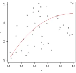
To illustrate the benefit of using a constrained estimator, in Figure 2.1, we consider an
increasing-concave function m(x) = 0.5x2log(x)−1.75x2+ 3x which is displayed as the solid curve, along with a set of observed data simulated from model (2.1) with errorsi iid∼N(0,0.5). Without any background knowledge about the underlying regression function the scatter plot
apparently might suggest a linear increasing regression function, and the least squares estimate
of such a line is displayed as the dotted line. Later in Section 2.4.2 we revisit this simulated
data example and show the substantial improvements in the fit brought by the subject matter
knowledge of an increasing concave function.
[insert Figure 2.1 here.]
Over the past decades, a lot of efforts have been devoted to search for a smooth and
com-putationally efficient nonparametric estimator of a regression function satisfying a desired set
of shape restrictions. Brunk (1955) first proposed a method based on estimating a step
func-tion subject to restricfunc-tions on the steps using the maximum likelihood method. Barlow et al.
(1972) proposed the so-called Pool Adjacent Violators Algorithm (PAVA) and a variety of the
Mukerjee (1988); A¨ıt-Sahalia and Duarte (2003) among others). In addition, several additional
efforts have been made to enrich the literature of estimating a monotone regression function
using other approaches, including the smoothing spline methods (Ramsay 1988; Mammen et
al. 2001; Wang and Li 2008), projection methods (Mammen et al. 2001), polynomial basis
estimators (Chang et al. 2007), and many alike. Hildreth (1954) pioneered the constrained least
squares method to estimate a concave function, and Wu (1982) and Fraser and Massam (1989)
proposed efficient algorithms to compute the estimator. A¨ıt-Sahalia and Duarte (2003) have also
considered a decreasing and convex function with certain bounds on the derivative. Hanson and
Pledger (1976), Mammen (1991) and Groeneboom et al. (2001) derived several asymptotic rate
of convergence. Alternative approaches which combine shape restriction and smoothing process
have also been proposed; for example, kernel-based estimators (Hall and Huang 2001; Dette
et al. 2006; Birke and Dette 2007), spline-based estimators (Pal, Woodroofe and Meyer 2007;
Meyer 2008), and polynomial-based estimators (Chang et al. 2007; Curtis and Ghosh 2011).
However, Birke and Dette (2007) pointed out the estimators produced by the constrained
least squares techniques and other projection based techniques may suffer from a lack of
smooth-ness, even when the underlying regression function is known to be smooth. In particular, those
estimators that rely on the PAVA algorithm often exhibit a step function like behavior when the
observations seem to be partitioned into groups. In addition, some of these estimators suffer
from the computational challenges especially when the sample sizes are large. For example, the
least squares based convex estimators in Dykstra (1983) and Han (1988) are usually computed
using iterative loops. Moreover, a few methods are believed to be too time consuming when
the sample sizes are extraordinarily large (e.g., sample sizen >10,000). For instance, the
esti-mator proposed by A¨ıt-Sahalia and Duarte (2003) requires one to construct restrictions at each
individual observed data point, and thus the number of constraint conditions could be as large
as the sample size. Another major drawback of these methods is that many of these estimators
are guaranteed to satisfy the given shape constraint only at observed x-values and not
be violated for values of the predictor variable which are not in the vicinity of the observed
data. The constrained least squares based estimators in Hildreth (1954) and Brunk (1955) are
commonly known to suffer from this crucial deficiency. Villalobos and Wahba (1987) proposed
a bivariate spline smoother which enforces the constraints on a grid of points. Mammen et al.
(2001) pointed out that the fitted spline smoother obtained by this estimation method would
not be guaranteed to satisfy the shape constraints everywhere in the domain of the predictor
space. We also observed from their numerical results (see Figures 3 and 4 in Villalobos and
Wahba (1987)) that some fitted smooth surface areas outside of the grid points violate the
concave assumption in they coordinate.
We adopt the method of sieve and propose an estimator based on restricted Bernstein
poly-nomials. The Bernstein polynomial is appropriate for shape-preserving regression, as it has the
optimal shape restriction property among all polynomials (Carnicer and Pena 1993), and all of
its derivatives possess the same convergence properties (Lorentz 1986). Moreover, the class of
Bernstein polynomials is dense (with respect to sup-norm) in the function space of all continuous
functions with compact support. When the true function has sufficient smoothness, Bernstein
polynomial and B-splines perform equivalently in terms of asymptotic properties. However,
there are at least two advantages of Bernstein polynomial. First, using Bernstein polynomial,
we are able to convert a fairly general shape restricted functional regression problem into a
(finite-dimensional) least squares problem with (only) linear constraint (for a multitude of
dif-ferent shapes) which can be solved easily using well established quadratic programming method.
Secondly, in our theory, higher order smoothness conditions are not required to establish
asymp-totic properties of the estimator. We only need the underlying true regression function to be
continuous (and may not be even be first order differentiable), which is in sharp contrast to
the assumptions that are generally used for B-splines theory. In addition, even if the function
is discontinuous of finite pointwise type, we can still use Bernstein polynomial to estimate the
regression curve (Herzog and Hill 1946).
curve estimation in Chak, Madras and Smith (2005); Chang et al. (2007); Curtis and Ghosh
(2011) and Stadtmuller (1986) among others. We build on these works and extend the
method-ologies to obtain a shape-restricted Bernstein polynomial estimator. There are several
advan-tages of our new estimator: Our estimator can be easily adapted to accommodate various
popu-lar shape constraints (such as nonnegativity, monotonicity, convexity, and increasing-concavity
and their variations and combinations). Our proposed estimator is guaranteed to satisfy the
required shape constraints everywhere in the domain of the predictor variable, including all
prediction points and not just at observed points. The method is computationally efficient,
because the proposed estimator can be easily computed as a solution of a quadratic
program-ming problem. Finally, under some mild regularity conditions, our estimator is shown to be
universally consistent.
The chapter is organized as follows. Section 2.2 presents the sieve-based Bernstein
polyno-mial estimator subject to a class of popular shape constraints and hence demonstrates how to
construct proper sieves corresponding to various shape restrictions, and concludes with
compu-tational details. In Section 2.3, we provide the asymptotic properties of the proposed estimator.
The corresponding proofs of our main results are provided in the Appendix. Section 2.4 presents
simulation studies when the underlying regression curve is subject to various shape constraints
such as monotonically increasing, concave or both. The numerical performance of our approach
is thoroughly examined and compared with a few currently available nonparametric regression
estimators subject to shape restrictions. In Section 2.5, we apply the proposed methodology on
real data sets and compare its predictive performance with other available methods. Finally, in
Section 2.6, we conclude with a brief discussion of our findings and future research directions.
2.2
Restricted Bernstein Polynomial Estimator
Consider again Dn ={(X1, Y1), ...,(Xn, Yn)} to be a set of observations which are assumed to be independently and identically distributed (i.i.d) as (X, Y) satisfying the regression model
a given class of shape restrictions. The regression function m(·) is the one that minimizes the L2 risk withinF (Gyorfi et al. 2002), i.e.,
m(·) = arg min f∈F
E{(f(X)−Y)2}. (2.2)
Throughout the chapter, we assume that predictor variables are suitably transformed to lie
in the unit [0,1] (see Section 2.2.2 for more computational details). Adopting the method of
sieves, we consider the constrained Bernstein polynomial sieve {FN} as follows:
FN ={BN(x) = N
k=0
βk·bk(x, N) :ANβN ≥0 and N
k=0
|βk| ≤LN}, (2.3)
for N = 1,2,· · ·, where bk(x, N) = N
k
xk(1 −x)N−k are the Bernstein basis polynomials. Notice that we can express BN(x) = bN(x)βN where bN(x) = (b0(x, N), ..., bN(x, N)) and
βN = (βN,0, ..., βN,N). For a vector b, we use b ≥ 0 to denote the fact that the inequality is satisfied componentwise. We allow the order of the polynomial, N to grow with the sample
size n, e.g.,N =o(nk) with a suitably chosenk >0, and the bound LN >0 is chosen suitably
to grow with N (see Main Theorem). AN represents a full row rank restriction matrix with dimensionRN ×(N + 1) whereRN denotes the rank ofAN. The matrixAN is chosen such a way that each (function) member in the sieveFN preserves the desired shape restrictions (i.e.,
FN ⊆ F,∀N). Given the data set Dn, the estimator mN, which is selected among all possible functions in FN, minimizes the empiricalL2 risk. That is:
mN(·) =bN(x) ˆβN where ˆβN = arg min βN∈BN
1 n
n
i=1
(bN(Xi)βN−Yi)2, (2.4)
whereBN ={βN ∈RN+1:ANβN ≥0, N
0 |βk| ≤LN}. Note that the existence ofmN follows
2.2.1 Examples of Constraint Bernstein Polynomial Sieves • Nonnegative Restriction
Let m(x) be a univariate function in the parameter space F = {f ∈ C[0,1] : f(x) ≥ 0,∀x ∈ [0,1]}, where C[0,1] denotes the space of all real-valued continuous functions defined on [0,1]. We define the restriction on the coefficients as follows:
ANβN ≡ ⎛ ⎜ ⎜ ⎜ ⎜ ⎜ ⎜ ⎜ ⎝
1 0 ... 0
0 1 ... 0
..
. ... . .. ...
0 0 ... 1
⎞ ⎟ ⎟ ⎟ ⎟ ⎟ ⎟ ⎟ ⎠ ⎛ ⎜ ⎜ ⎜ ⎜ ⎜ ⎜ ⎜ ⎝ β0 β2 .. . βN ⎞ ⎟ ⎟ ⎟ ⎟ ⎟ ⎟ ⎟ ⎠ ≥ ⎛ ⎜ ⎜ ⎜ ⎜ ⎜ ⎜ ⎜ ⎝ 0 0 .. . 0 ⎞ ⎟ ⎟ ⎟ ⎟ ⎟ ⎟ ⎟ ⎠ .
Clearly in this caseAN =IN+1, the identity matrix of order (N+ 1) and its rankRN = N+ 1. The above restriction ensuresβk ≥0, for allk. Since Bernstein basis polynomials bk(x, N) =
N k
xk(1−x)N−k are always nonnegative,BN(x)≡Nk=0βk·bk(x, N) are also nonnegative. This impliesFN ⊂ F.
• Monotone Restriction
Without loss of any generality, a monotone function in this chapter refers to a
non-decreasing function. Non-increasing monotonicity can be simply obtained by reversing
the inequalities. Let m(x) be a real-valued monotone function in the space F = {f ∈ C[0,1] :f(x1)≤f(x2),∀0≤x1≤x2≤1}whereC[0,1] denotes the class of all continuous functions defined on [0,1]. FN is the sieve defined in (2.3) and the increasing monotonicity is satisfied by the following conditions:
ANβN ≡ ⎛ ⎜ ⎜ ⎜ ⎜ ⎜ ⎜ ⎜ ⎝
−1 1 0 ... 0
0 −1 1 0 ...
. . .
0 ... 0 −1 1
⎞ ⎟ ⎟ ⎟ ⎟ ⎟ ⎟ ⎟ ⎠