18th International Conference on Structural Mechanics in Reactor Technology (SMiRT 18) Beijing, China, August 7-12, 2005 SMiRT18-M04-2
PROBABILISTIC FRAMEWORK FOR THE ASSESSMENT OF
STRUCTURES SUBMITTED TO THERMAL FATIGUE
Bruno Sudret
Electricité de France – R&D division
Site des Renardières
F-77818 Moret-sur-Loing Cedex
Phone: +33 1 60 73 77 48
Fax: +33 1 60 73 65 59
E-mail: [email protected]
ABSTRACT
A probabilistic framework is set up to assess the fatigue life of components of nuclear power plants. It intends to incorporate all kinds of uncertainties such as those appearing in the specimen fatigue strength (number-of-cycles-to-failure of specimens), design margin factors (taking into account the size, surface finish and environmental effects), mechanical model (precisely, the uncertainty on the model input parameters) and the thermal loading. A comprehensive example involving a mechanical model of a pipe submitted to a deterministic inner temperature is analyzed. The use of the First Order Reliability Method (FORM) allows to compute the probability of failure as a function of the foreseen life time and to rank the input random variables according to their importance in response sensitivity.
Keywords:
Uncertainties, Thermal fatigue, Structural reliability, FORM/SORM, Sensitivity analysis
1. INTRODUCTION
A number of components in nuclear power plants are submitted to thermal and mechanical loading cycles. The assessment of these components with respect to low cycle and high cycle fatigue is of great importance for the global safety, efficiency and availability of the power plant. The French assessment rules, which are codified in a design code called RCC-M (AFCEN, 2000) are fully deterministic in nature. However, it is well known that various sources of uncertainty affect the behaviour of structures submitted to fatigue, namely:
• The scatter of the results observed when fatigue tests are carried out onto a set of identical samples (same material, same loading conditions, same environment, etc.), see Shen et al. (1996);
• The size effect, surface finish effect and environmental effect (temperature, oxygen content in the PWR environment), which globally reduce the fatigue life time of a real structure (Coll. Framatome, 1998; Rosinsky, 2001). In the codified design, the so-called margin factors are applied to the “best-fit” experimental curve in order to obtain the design fatigue curve, i.e. to compute the number-of-cycles-to-failure of a structure in its operating conditions from the number-of-cycles-to-failure of a specimen tested in the laboratory. These factors denoted hereinafter by
,
N S
• The imprecision in the mechanical model that yields the stress cycles amplitudes. Often the model may be quite accurate per se, whereas the input parameters (e.g. material properties) are not well known, while they have a great influence on the mechanical response. Moreover, in the specific case of thermal fatigue due to thermal fluctuations in PWR circuits, the loading may not be well known either;
• The imprecision in evaluating the cumulated damage, using for instance Miner’s rule of linear damage accumulation.
In this context, it appears interesting to introduce explicitly the uncertainties in fatigue analysis through a rigorous probabilistic modelling of all uncertain input quantities, and study their influence onto the output (e.g.
the cumulated damage D). This cumulated damage indeed becomes a random variable itself in the probabilistic context, which depends on all input random variables and can be characterized in terms of mean and standard deviation. The latter corresponds to the scattering of life time of identical components that could be observed in a fleet of identical PWR.
From the point of view of reliability analysis, it will be possible to compute the probability of failure with respect to crack initiation, i.e. the probability that the cumulated damage is greater than 1 for a prescribed operating duration.
The deterministic framework used for fatigue assessment of nuclear components is first recalled (in a simplified manner) in Section 2. The various sources of uncertainty that have been mentioned above are then listed and a suitable probabilistic model is proposed for each of them in Section 3. The formalism of structural reliability analysis is then recalled in Section 4. Finally an application example concerning the probabilistic fatigue assessment of a pipe is proposed in Section 5.
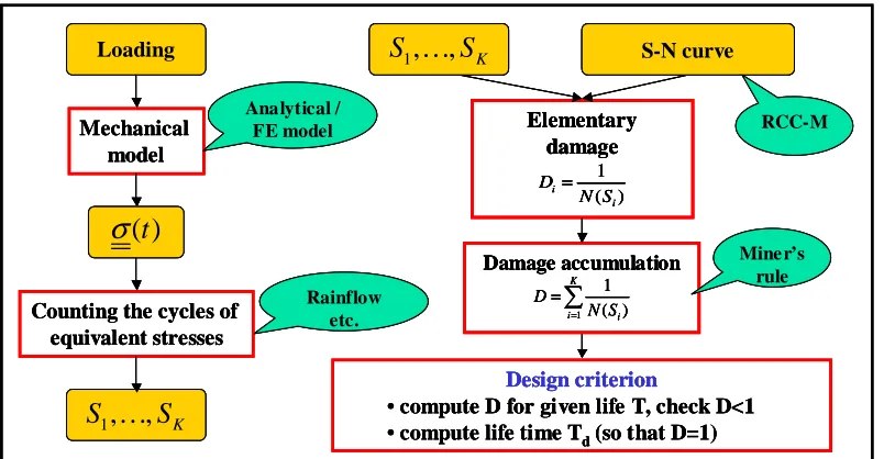
2. DETERMINISTIC FRAMEWORK FOR FATIGUE ASSESSMENT
The assessment of structural components such as pipes against thermal fatigue requires the following inputs: • Description of the loading applied to the component: the temperature history applied onto the
inner wall of the pipe is given e.g. from a thermo-hydraulic calculation, experimental data obtained from scaled models or in situ measurements.
• Mechanical model: it allows to compute the evolution in time of the stresses in each point of the component. The input parameters are the geometry (e.g. pipe radius and thickness), the material properties (e.g. Young’s modulus, Poisson’s ratio, coefficient of thermal expansion) and fluid/structure boundary conditions (e.g. fluid temperature history and heat transfer coefficient). Analytical or numerical (e.g. finite element) models can be used. An equivalent stress σeq( )t is then obtained using for instance the Tresca criterion.
• Extraction and counting of the cycles: from the computed evolution σeq( )t , stress cycles are extracted using the Rainflow method (Amzallag et al., 1994). A sequence of stress amplitudes
, 1, i
S i= N can be determined on a time interval (each stress amplitude Si corresponds to half of the difference between the consecutive peaks obtained by the Rainflow method).
• Choice of a design curve: as described in the introduction, the design curve Nd( )S is obtained from experimental results that provide the best-fit specimen curve Nb f (S) , and from margin factors (γN = 20 on number of cycles, γS = 2 on stress, whichever is more conservative).
• Computation of the cumulated damage: The Miner’s rule (linear damage accumulation) is used in order to estimate the fatigue damage. It postulates that the elementary damage di associated with one cycle of amplitude Si is computed by di =1 /Nd( )Si (where Nd( )S is the design curve) and
that the total damage is obtained by summation. This leads to compute the cumulated damage (or usage factor) D by:
1 1
1/
( )
N N
i d i i i
D
d
N S
= =
=
∑ ∑
=
(1)Elementary damage 1 ( ) i i D N S = Design criterion
•compute D for given life T, check D<1
•compute life time Td(so that D=1) Loading
Mechanical model
Analytical / FE model
( )
t
σ
Counting the cycles of equivalent stresses
1
,
,
KS
…
S
Rainflow etc.
1
,
,
KS
…
S
S-N curveRCC-M Damage accumulation 1 1 ( ) K i i D N S = =
∑
Mine r’s rule Elementary damage 1 ( ) i i D N S = Elementary damage 1 ( ) i i D N S = Elementary damage 1 ( ) i i D N S = Design criterion•compute D for given life T, check D<1
•compute life time Td(so that D=1)
Design criterion
•compute D for given life T, check D<1
•compute life time Td(so that D=1) Loading Mechanical model Analytical / FE model Loading Mechanical model Analytical / FE model
( )
t
σ
Counting the cycles of equivalent stresses
1
,
,
KS
…
S
Rainflow etc.
( )
t
σ
( )
t
σ
Counting the cycles of equivalent stresses
1
,
,
KS
1,
…
,
S
KS
…
S
Rainflow etc.
1
,
,
KS
…
S
S-N curveRCC-M
1
,
,
KS
1,
…
,
S
K S-N curveS
1,
…
,
S
KS
…
S
S-N curveS-N curveRCC-M Damage accumulation 1 1 ( ) K i i D N S = =
∑
Mine r’s rule Damage accumulation 1 1 ( ) K i i D N S = =∑
Damage accumulation 1 1 ( ) K i i D N S = =∑
Mine r’s ruleFig. 1: Flow chart of the deterministic fatigue assessment
3. PROBABILISTIC REPRESENTATION OF THE INPUT DATA AND THE CUMULATED DAMAGE 3.1 Thermal loading
The temperature of the fluid at the inner wall of the pipe may be represented either by:
• a deterministic signal obtained from measurements (in situ or from scale models) or a thermo-hydraulic computation (Benhamadouche et al., 2003),
• a random process, which is supposed Gaussian and stationary due to the periodicity in the circuit operating. Generally speaking, this process may be indexed on both time and space coordinates. In order to be handled in the calculation, the process has to be discretized either in the time domain (generation of trajectories) or in the frequency domain (using the power spectral density). This point will not be elaborated in the present paper, see Guédé et al. (2004) for a comprehensive presentation.
3.2 Mechanical model
The mechanical model allows to compute the history of the stress tensor from the geometry, material properties and loading parameters. Its complexity can vary from low (e.g. analytical one-dimensional formulation) to high (e.g. three-dimensional non linear finite element analysis). In the sequel, the finite difference code OSTAND developed by EDF R&D will be used. It allows to solve one-dimensional axisymmetrical problems.
From the probabilistic point of view, all the input parameters of the code can be considered as random variables, including geometrical characteristics (e.g. pipe radius and thickness), material properties (e.g. Young’s modulus, Poisson’s ratio, thermal expansion coefficient) and fluid/structure boundary conditions (e.g. fluid temperature history and heat transfer coefficient). Each random variable is defined by its probability density function (PDF) and the related parameters.
3.3 Scatter of the fatigue test results
The number-of-cycles-to-failure observed in a set of specimens made of the same materials tested in the same experimental conditions (same alternate stress, strain ratio, etc.) shows a significant scatter. This scatter is all the larger since the alternate stress S is close to the endurance limit. The number-of-cycles-to-failure at a given alternate stress S is thus represented by a random variable N S
(
,ω)
, where ω denote the randomness. The statistical analysis used in order to characterize properly this random variable has been presented in Sudret et al.For each stress amplitude S, the number-of-cycles-to-failure N S
(
,ω)
is supposed to follow a lognormaldistribution (its logarithm is supposed to be normally distributed), whose mean and standard deviation are dependent on S. Moreover, it is assumed that these random variables N S
(
,ω)
are perfectly correlated whatever the stress level S. This corresponds to the heuristic assumption that a given sample (which is arealization of the material in the probabilistic context) is globally “well” or “bad” resistant to fatigue crack initiation whatever the applied stress. Unfortunately this assumption cannot be verified since only one test at a given stress level can be carried out (then the sample is broken and cannot be tested at another stress level). These assumptions lead to write:
(
)
lnN S,ω =λ( )S +ς( ) ( )S ξ ω (2)
where λ( )S and ς( )S are the mean and standard deviation of lnN and ξ is a standard normal random variable. The model for the median curve is based on the work by Langer (1962). The data observation leads to consider the standard deviation ς( )S as proportional to the medium curve (heteroscedastic assumption). Thus:
(
)
( )S Aln S SD B
λ = − +
ς
( )S =δ λ
( )S (3)The median S-N curve and its scattering are thus fully characterized by four parameters, namely A B S, , D,δ , which are evaluated using the maximum of likelihood method.
3.4 Specimen/structure passage factors
As described above, each of the design margin factors
(
γ
N=
20 ;
γ
S=
2
)
can be decomposed into a product of two sub-factors.N N N scat passage S S S
scat passage
γ
γ
γ
γ
γ
γ
=
⋅
=
⋅
(4)In this expression,
γ
scatN,
γ
Npassage respectively denote:• a subfactor taking into account the scatter of the test results, e.g. 2 on
γ
N=
20
and 1.19 on2
S
γ
=
(Coll. Framatome, 1998),• a specimen-to-structure passage factor taking into account the reduction of fatigue life of a real component in its environment compared to a specimen made of the same material tested in the laboratory. This global passage factor is the product of the size effect, the surface finish and the environment- subfactors.
In the present probabilistic framework, the scatter of the number-of-cycles-to-failure of the specimens is already described by the very definition of random variable N
( , )
S
ω
. Passage factors are also considered as random variables, whose parameters are yet to be defined, e.g. from experiments carried out both on specimen and scaled structures and comparison thereof.3.5 Random elementary- and cumulated damage
According to the above assumptions, the elementary damage d S( , )ω underwent by a structure submitted to a cycle S is a random variable defined by:
( , ) 1 / min ( , ) / Npassage, ( Spassage , )
d S ω =
N S ω γ N γ S ω
(5)Using Miner’s rule, the cumulated damage is also a random variable depending on all the input random variables described above:
1
( ) ( , )
N
i i
Dω d S ω
=
=
∑
(6)4. RELIABILITY ANALYSIS 4.1 Problem statement
Structural reliability analysis aims at computing the probability of failure of a mechanical system with respect to a prescribed failure criterion by accounting for uncertainties arising in the model description (geometry, material properties) or the environment (loading). Let us denote by
X
( )
ω
=
{
X
1( ),
ω
X
2( ),...,
ω
X
n( )
ω
}
the set of random variables describing the randomness in the geometry, material properties and loading. The failure criterion under consideration is mathematically represented by a limit state function
g X
( )
defined in the space of parameters as follows :•
g X
( )
>
0
defines the safe state of the structure.•
g X
( )
≤
0
defines the failure state. In the present paper, the failure state will be related to crack initiation, i.e. to the fact that the cumulated damage is greater than 1.•
g X
( )
=
0
defines the limit state surface.Denoting by
f
X( )
x
the joint probability density function of random vectorX
, the probability of failure of the structure is :( ) 0
( )
f X
g x
P
f
x d x
≤
=
∫
(7)In all but academic cases, this integral cannot be computed analytically. Indeed, the failure domain is often defined by means of response quantities (e.g. displacements, strains, stresses, etc), which are computed by means of computer codes (e.g. finite element code) in industrial applications, meaning that the failure domain is
implicitly defined as a function of X. Thus numerical methods have to be employed.
Monte Carlo simulation is a universal method for evaluating integrals such as in Eq.(7). Denoting by
[ ( ) 0]
1
g x≤( )
x
the characteristic function of the failure domain (i.e. the function that take zero value outside thefailure domain and 1 inside), Eq.(7) rewrites:
[ ( ) 0] [ ( ) 0]
1
( )
( )
E 1
( )
n
f g x X g x
P
=
∫
≤x f
x d x
=
≤x
(8)In this expression,
E .
[ ]
denotes the mathematical expectation. Practically, Eq.(8) can be evaluated by simulating realizations of the random vector X, say{
(1),
,
(Nsim)}
X
X
. For each sample,g X
( )
( )i is evaluated. An approximation of Pf is given by:( ) [ ( ) 0] 1
1
(
)
sim
N
i fail f g x
i sim
N
P
X
N
≤ =
≈
∑
=
(9)where Nfail denotes the number of samples that are in the failure domain. As mentioned above, Monte Carlo simulation is applicable whatever the complexity of the deterministic model. However, the number of samples
Nsim required to get an accurate estimation of Pf may be dissuasive, especially when the value of Pf is small.
4.2 FORM method
The First Order Reliability Method has been introduced to get an approximation of the probability of failure at a low cost (in terms of number of evaluations of the limit state function), see Ditlevsen and Madsen (1996). The first step consists in recasting the problem in the standard normal space by using a probabilistic transformation
X
→ =
U
T X
( )
. The Rosenblatt or Nataf transformations may be used for this purpose. Thus Eq.(7) rewrites:1 ( ) 0 ( ( )) 0
( ) ( )
f X n
g x g T u
P f x d x
ϕ
u d u −≤ ≤
=
∫
=∫
(10)( )
(
12 2)
1 1
( ) exp
2 2
n u n u un
ϕ
π
= − + + (11)
This PDF is maximal at the origin and decreases exponentially with
u
2. Thus the points that contribute at most to the integral in Eq.(10) are those of the failure domain that are closest to the origin of the space.The second step in FORM thus consists in determining the so-called design point, i.e. the point of the failure domain closest to the origin in the standard normal space. This point P* is obtained by solving an optimisation problem :
(
)
{
}
* 1
*
min
/
( )
0
P
=
u
=
Arg
u
g T
−u
≤
(12)Several algorithms are available to solve the above optimisation problem, e.g. the Abdo-Rackwitz or the SQP (sequential quadratic programming) algorithm (Ditlevsen and Madsen, 1996). The corresponding reliability index is defined as :
* 1
sign
g T
(
(0))
u
β
=
−
⋅
(13)It corresponds to the algebraic distance of the design point to the origin, counted as positive if the origin is in the safe domain, or negative in the other case.
The third step of FORM consists in replacing the failure domain by the half space HS(P*) defined by means of the hyperplane which is tangent to the limit state surface at the design point. This leads to :
1 ( *)
( ( )) 0
( )
( )
f n n
HS P g T u
P
ϕ
u d u
ϕ
u d u
− ≤
=
∫
≈
∫
(14)The latter integral can be evaluated in a closed form and gives the first order approximation of the probability of failure :
( )
( )
2/ 2,
1
;
2
x x
f f FORM
P
P
β
x
e
dx
π
− −∞
≈
= Φ −
Φ
=
∫
(15)where Φ(x) denotes the standard normal cumulative distribution function(CDF). The unit normal vector
*
/
u
α
= −
β
allows to define the sensitivity of the reliability index β with respect to each variable. Precisely the squared componentsα
i2ofα
(which sum up to one) are a measure of the importance of each variable in the computed reliability index (Ditlevsen and Madsen, 1996).In this study the probabilistic code PROBAN (Det Norske Veritas, 2001) is used to solve the optimisation algorithm associated with FORM. When the quantities involved in the limit state function are obtained numerically, a coupling between this code and the deterministic code has to be implemented. This is performed by the implementation of a FORTRAN routine g.f that computes the value of g from the current values of the design parameters by running OSTAND and post-processing the results.
5. APPLICATION EXAMPLE TO A PIPE 5.1 Problem statement
0 50 100 150 200 250
0 1 2 3 4 5
Temps (s)
Tem
p
ér
at
ur
e (
°C)
Fig.2 : Fatigue analysis of a pipe: fluid temperature history
5.2 Mechanical model
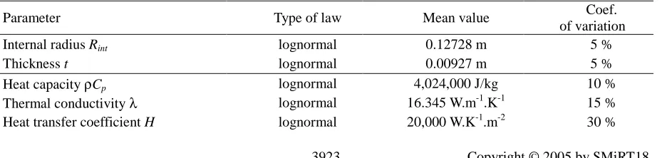
Let us consider a typical section of a straight portion of the circuit. Due to symmetry, the one-dimensional axisymmetric model (as implemented in the finite difference code OSTAND) is relevant to compute the stress history. The simulation assumes generalized plane strain conditions (strain component εzz is supposed constant throughout the pipe thickness and is an unknown of the problem). Geometry and material properties are gathered in Table 1.
Due to the peculiar geometry of the problem, the stress tensor is diagonal in the natural coordinate system
(
r
, ,
θ
z
)
. The stress componentσ
rr due to thermal loading is zero at the inner wall, whereas the two other components are equal(
σ
θθ=
σ
zz)
. This means that the three-dimensional stress state is completely described by a scalar stress historyσ
θθ( )
t
, from which the stress cycles can be easily obtained using the Rainflow counting method.5.3 Deterministic fatigue analysis
The fatigue behavior of the material of the pipe under consideration is supposed to be described by the expressions derived in Section 3, where the parameters have been identified on a set of 304L austenitic stainless steel samples (see Sudret et al., 2003). Thus the best-fit curve (median value) of the number-of-cycles-to-failure is ( ) exp
(
2, 28 ln( 185, 9) 24, 06)
bf
N S = − S− + . A thermo-mechanical analysis using OSTAND together with
the mean values of the parameters (See table 1, column #3) is first carried out. The Rainflow counting provides 33 cycles, from which 2 are leading to elementary damage : S1=102.1 MPa , S2=190.6 MPa. Accordingly, the cumulated damage associated to one sequence of loading is 5.98 10-6. Thus the codified design gives a life time of
N
seqdet= 1/5.98 10-6 = 167,200 sequences.5.4 Probabilistic analysis
The parameters of the thermo-mechanical analysis are now described in terms of random variables. The choice of the probability density functions is dictated by common practice. The mean value and coefficient of variation of each parameter is given in Table 1.
Table 1 : Fatigue analysis of a pipe: input random variables
Parameter Type of law Mean value Coef.
of variation
Internal radius Rint lognormal 0.12728 m 5 %
Thickness t lognormal 0.00927 m 5 %
Heat capacity ρCp lognormal 4,024,000 J/kg 10 %
Thermal conductivity λ lognormal 16.345 W.m-1.K-1 15 %
Young’s modulus E lognormal 189,080 MPa 15 %
Poisson’s ratio ν bêta [0 ; 0,5] 0.3 10 %
Thermal expansion coefficient α lognormal 16.95 10-6 10 %
Passage factor
γ
passageN [0 ; 20] 10 20 %Passage factor
γ
Spassage bêta [0 ; 2] 1.68 20 %Fatigue strength scatter ξ (Eq.(5)) normal 0 Std. Dev. : 1
The number-of-cycles-to-failure of the specimen is represented by a lognormal random variable according to the results in Section 3 with the following parameters : A= −2.28 ; B=24.06 ; SD =185.9 ; δ =0.09. This corresponds to:
(
)
(
( )
)
[
]
( , ) exp 2, 28 ln( 185, 9) 24, 06 1 0, 09
N S
ω
= − S− + +ξ ω
(16)where ξ ω
( )
is a standard normal random variable. The passage factors yielding the number-of-cycles-to-failure of the structure are represented by random variables following a bêta distribution whose mean value are respectively 20/2 = 10 (low cycle domain) and 2/1,19 = 1,68 (high cycle domain) and 20 % of coefficient of variation.Using this probabilistic input, it is possible to characterize the randomness of the cumulated damage for a given life time, say 100,000 sequences of operating. The latin hypercube sampling technique was applied using 100 samples. The mean value and standard deviation of the cumulated damage are 0.921 and 2.00 respectively, hence a coefficient of variation of 217 %. It is clear from this analysis that the large scatter of the fatigue strength in the limited endurance domain yields a large scatter in the fatigue life time of the structure. The approach allows to quantify the latter properly.
The reliability of the structure under consideration may now be studied as a function of the number of sequences of operating Nseq. The limit state function is defined by:
(
seq,
( )
)
1
seq seq( ( ))
g N
X
ω
= −
N d
X
ω
(17)In this expression, vector
X
( )
ω
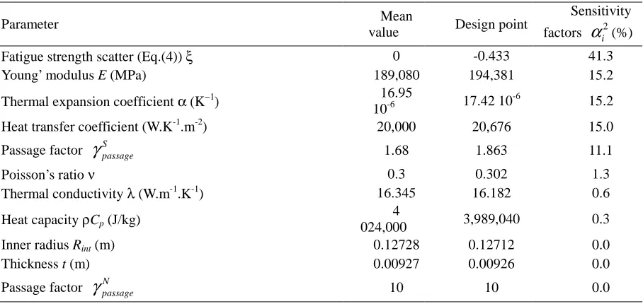
gathers all the input random variables as reported in Table 1. FORM analysis is used to compute the reliability index and the probability of failure. For Nseq = 100,000 sequences, the results are:β
=
0.68 ;
P
f=
0.249
. The coordinates of the design point (back-transformed to the physical space) as well as the sensitivity factors are reported in Table 2.It is observed that the uncertainty related to the fatigue strength of the material here again is the most important factor driving the reliability of the structure. Variable ξ is of course a “resistance” variable since its design point value is below the mean value. Then there are the Young’s modulus and coefficient of thermal expansion (which transform cycles of temperature in the pipe into stress cycles), the heat transfer coefficient (which transforms the fluid temperature peaks into the pipe inner wall temperature peaks) and finally the passage factor
γ
Spassage. These four variables are “demand” variables since their value at design point is above the mean value. All other random variables have negligible sensitivity factors: this means that they could be considered asdeterministic in this kind of analysis. Note that the passage factor
γ
passageN has zero importance in the present example because it does not enter the analysis at all: the obtained stress cycles are sufficiently small so that only the “high cycle passage factor”γ
Spassage is used.0 0,2 0,4 0,6 0,8 1 1,2 1,4 1,6 1,8 2
0 50000 100000 150000 200000
Nombre de séquences (Nseq)
In
d
ice
d
e
fia
b
ilité
b
0 0,05 0,1 0,15 0,2 0,25 0,3 0,35 0,4 0,45 0,5
P
rob.
de déf
ai
llanc
e
Indice de fiabilité Prob. de défaillance
Fig.3 : Fatigue analysis of a pipe: reliability index (resp. the probability of failure) vs. life time Nseq
Table 2 : Fatigue analysis of a pipe: probabilistic results for Nseq = 100,000 séquences
Parameter Mean
value Design point
Sensitivity factors
α
i2(%)Fatigue strength scatter (Eq.(4)) ξ 0 -0.433 41.3
Young’ modulus E (MPa) 189,080 194,381 15.2
Thermal expansion coefficient α (Κ−1) 16.95
10-6 17.42 10
-6 15.2
Heat transfer coefficient (W.K-1.m-2) 20,000 20,676 15.0
Passage factor
γ
Spassage 1.68 1.863 11.1Poisson’s ratio ν 0.3 0.302 1.3
Thermal conductivity λ (W.m-1.K-1) 16.345 16.182 0.6
Heat capacity ρCp (J/kg)
4
024,000 3,989,040 0.3
Inner radius Rint (m) 0.12728 0.12712 0.0
Thickness t (m) 0.00927 0.00926 0.0
Passage factor
γ
passageN 10 10 0.06. CONCLUSIONS
Fatigue analysis of structural components in nuclear power plants is of crucial importance. The fatigue phenomenon is by nature random due to the mechanisms responsible for crack initiation which take place at microscopic scale. The present paper proposes a probabilistic framework of analysis which aims at incorporating in a rigorous manner all kinds of uncertainties appearing in the fatigue assessment.
In order to be easily understood by practitioners, the usual assessment rules codified in the French regulatory guide have been taken as a base line. In each step, sources of uncertainty have been identified and a probabilistic model has been proposed.
Introducing all these random variables as input makes the cumulated damage (which is an indicator of fatigue crack initiation) random. Its randomness can be characterized a) in terms of mean value and standard deviation b) in terms of probability of exceeding the threshold 1.
The pipe application example provides additional useful insight on the fatigue design. The first analysis shows that the coefficient of variation of the cumulated damage is rather high (217 % in the application example). Hence the well-known randomness on the fatigue life time of a structure in the high cycle domain is quantified.
Reliability index Probability of failure
Number of sequences Nseq
Note that the weight of each parameter in the total variance could be computed easily using e.g. the perturbation method.
The reliability analysis allows to compute the probability of failure corresponding to crack initiation. Sensitivity factors related to the use of FORM analysis may also be computed. They allow to rank the input random variables according to their weight on the computed reliability index. Five important variables have been identified by this method, namely the fatigue strength of the material, the Young’s modulus and coefficient of thermal expansion, the heat transfer coefficient at the pipe inner wall and finally the passage factor
γ
passageS . The other random variables (termed as “unimportant” from a probabilistic point of view) may be considered as deterministic in subsequent analysis. Note that the very values of the sensitivity factors should be taken with caution since they truly depend on the choice of the PDF of the input parameters (and also on their coefficient of variation).As a conclusion, the original result in this paper is the complete methodology for incorporating uncertainties in the codified fatigue assessment more than the various numerical results presented in Section 5. Indeed the parameters and laws of the input random variables have not been selected here after a true statistical analysis, but more on literature results and expert judgment. An important work on the input data remains for applying properly the methodology.
Simple models have been retained in all steps of the analysis for the application example (deterministic loading, thermo-mechanical 1D calculation, linear damage accumulation). More complex models can be easily integrated in the framework, including non linear two- or three-dimensional finite element models). The case of a random loading represented by a Gaussian random process has been dealt with in Guédé et al. (2004).The computation takes place in the frequency domain in this case. Due to linearity, it is possible to derive an analytical transfer function that yields the stress components as a function of the temperature at each frequency. This transfer function used together with the power spectral density of the fluid temperature provides the power spectral density of the stress. The latter is then transform into the probability density function of the stress amplitudes, which directly enters the probabilistic analysis. Details on this work can be found in Guédé (2004).
ACKNOWLEDGEMENT
The author would like to thank Mr Z. Guédé and Pr. M. Lemaire from the Institut Français de Mécanique Avancée (Clermont-Ferrand, France) for useful discussions around this topic, as well as Mr J.-M. Stéphan (EDF R&D) for his contribution to the work in terms of input data and critical comments.
REFERENCES
AFCEN, Règles de Conception et de Construction des Matériels des Ilots Nucléaires, (RCCM), Paris, Juin 2000.
Amzallag, C., Gerey, J.-P., Robert, J.-L. and Bahuaud, J., 1994. Standardization of the Rainflow counting method for fatigue analysis, Int. J. Fatigue, 16, 287-293.
Benhamadouche, S., Sakiz,M., Péniguel, C., Stéphan, J.-M., 2003. Presentation of a new methodology of chained computations using instationary 3D approaches for the determination of thermal fatigue in a T-Junction of a PWR Nuclear Plant, Trans. 17th Int. Conf. On Struct. Mech. in Reactor Tech. (SMiRT 17), Prague, Czech Republic.
Coll. Framatome, 1998. Re-evaluation of Fatigue Analysis Criteria, FRAMATOME report n°EE/S 98.317 (Final report to CEC-DG XI contract B4-3070/95/000876/MAR/C2).
Det Norske Veritas, 2002. Proban user’s manual.
Ditlevsen, O. and Madsen, H., 1996. Structural reliability analysis, J. Wiley.
Guédé, Z., Sudret, B. and Lemaire, M., 2004. Analyse fiabiliste en fatigue thermique, Proc. 23èmes Journées de Printemps – Commission Fatigue, « Méthodes fiabilistes en fatigue pour conception et essais », Paris. Langer, B. Design of pressure vessels for low-cycle fatigue, J. of Basic Eng., Trans. ASME, pp. 389-402, 1962. Shen, C.L., Wirsching, P.H. and Cashman, G.T, 1996. Design curve to characterize fatigue strength, J. Eng.
Mat. Tech., Trans. ASME, 118, 535-514.
Rosinski, S., 2001. Evaluation of fatigue data including reactor water environmental effects – Materials Reliability Project (MRP-54), EPRI report n° 1003079.