The effect of position along the chain on the dynamic properties
of hard chain segments
Julie A. McCormick, Carol K. Hall,a)and Saad A. Khan Department of Chemical Engineering, North Carolina State University, Raleigh, North Carolina 27695-7905
共Received 13 December 2001; accepted 12 April 2002兲
Discontinuous molecular dynamics simulations are performed on systems containing 32 hard chains of length 192 at three volume fractions,⫽0.40, 0.45, and 0.50, to investigate the effect of position on the segmental mean squared displacement. The mean squared displacements of various sized blocks of segments at different positions along the chain are calculated. First, the effect of block size on the dynamics of end and middle blocks is considered. It is found that small blocks provide a greater difference between the mean squared displacements of middle blocks, end blocks, and the whole chain than larger equal-sized blocks. Next, the portions of the chain exhibiting end and middle behavior are determined. It is found that a large portion of the chain displays middle behavior, while a small portion displays end behavior. Finally, the dynamics of segment relaxation along the chain are studied. The relaxation of small blocks of segments at different positions along the chain starts at the chain ends and progresses toward the chain middle with time, as the tube model predicts. The minor chain length, the portion of the chain that has relaxed, follows a power law with time, but the power is somewhat less than predicted. © 2002 American Institute of
Physics. 关DOI: 10.1063/1.1483295兴
I. INTRODUCTION
One way to evaluate the ability of theories like the Rouse,1reptation,2and tube3models to describe the dynamic behavior of entangled polymers is to test their predictions for the dependence of segmental dynamics on position along the chain against experimental data. Experiments4 – 6designed to compare the dynamics of blocks of segments in the center of a chain with those at the chain ends have been performed but were limited to large blocks or relatively short times, raising the question of whether this is sufficient to obtain a complete picture of the effect of chain position on the diffusion of chain segments. Although some simulations have been per-formed to study segmental dynamics as a function of posi-tion along the chain,7–17 most7–15 have focused on compar-ing the dynamics of segments in the chain middle to tube model predictions.
The aim of this study is to investigate the effect of the position along the chain on segmental dynamic behavior. We use discontinuous molecular dynamics computer simulations to study how the size of the block impacts conclusions drawn from comparing the dynamics of end segments to those of middle segments. The idea here is to see how small the blocks must be in order to distinguish the behavior of chain ends from that of the chain middle. Then, we determine the portion of the chain that exhibits chain middle behavior and the portions of the chain that exhibit chain end behavior. Finally, we investigate the dynamics of segment relaxation as a function of position along the chain to determine how the relaxation propagates along the chain.
Experimental studies4 – 6comparing the dynamics of end
blocks to that of middle blocks have employed the tech-niques of neutron spin echo 共NSE兲 spectroscopy, dynamic secondary ion mass spectroscopy, or specular neutron reflec-tivity. These techniques require the synthesis of labeled poly-mer samples in order to obtain dynamic information about specific sections along the chain. As described in detail be-low, the labeled end and middle blocks used in these studies have been relatively large, containing between 25% and 50% of the chain segments.
Ewen et al.4 performed NSE experiments to study seg-mental diffusion of entangled polydimethylsiloxane共PDMS兲 melts. Three separate samples of chains labeled by hydrogen–deuterium exchange were used to compare the motion of large middle chain sections共37%兲, large end chain sections共78%兲, and the entire chain. The tube diameter, dT,
which specifies the lateral constraints on the segments, was estimated for the chain middle, the chain ends, and the whole chain from the NSE experiments. They found that the lateral constraints were the same for the middle third of the chain, the outer third of the chain, and the whole chain.
Welp et al.5 investigated the interdiffusion of polysty-rene 共PS兲 chains during welding in the melt using dynamic secondary ion mass spectroscopy and specular neutron re-flectivity to obtain information about the microscopic details of polymer dynamics. In this study, they used bilayer samples made up of two layers of oppositely labeled PS triblock chains to compare the diffusion behavior of the chain ends to that of the chain middle. In one layer, the inner 50% was deuterium labeled, and in the other layer, the outer 25% on each end was deuterium labeled. The samples were welded for various annealing times in order to obtain the deuterium peak height, peak position, and the area under the a兲Author to whom correspondence should be addressed.
944
peak as a function of time. The Rouse model,1the polymer mode-coupling model,18 and reptation theory2,3 provide unique predictions for these quantities. Reptation theory pro-vided the best description of the interdiffusion results.
In a subsequent study, Welp et al.6studied the motion of central and end sections of polymers independently during interdiffusion experiments by using different samples to ob-serve the motion of each section directly. Specular neutron reflectivity was used to determine changes in the deuterium depth profile over time and thus the diffusion of a given chain section. Two different polymer bilayer samples were used to observe the motion of end sections and middle sec-tions independently. Each bilayer sample contained a layer of hydrogenated–deuterated–hydrogentated PS共HDH-PS兲 that was 50% hydrogenated PS and 50% deuterated PS. The other layer in the ends bilayer sample contained fully deuterated PS共D-PS兲, and the other layer in the center bilayer sample contained fully hydrogenated PS 共H-PS兲. The average pen-etration distances,
具
X(t)典
, of the ends and the centers were monitored. The experimental results were consistent with reptation predictions and inconsistent with Rouse predic-tions, the same as in previous work.The many experimental challenges associated with de-termining the diffusion of selected segments along the length of polymer chains may explain the relatively limited body of experimental work in this area. First of all, there is a need for specialized equipment. Very few neutron spectrometers exist, and thus obtaining sufficient beam time to perform the experiments can be a challenge in itself. Secondly, tailored materials or multiple experimental techniques may be needed to access all the time and length scales of interest. Finally, obtaining information about the diffusion of specific seg-ments along the chain requires the controlled synthesis of specially labeled polymers. This adds to the difficulty and cost of the experiments. An adequate portion of the material must be labeled to obtain a sufficient signal to noise ratio. Also, each chain section to be studied requires the synthesis of additional samples and the performance of additional experiments.
Computer simulation can provide new and complimen-tary information on the diffusion behavior of segments at different positions along the chain. Simulations do not require the preparation of a different system to study each section along the chain as is required during experiments; thus, a single simulation may provide information that would otherwise require many experiments. Also, following the motion of specific segments along the chain does not require that the chain be altered; in contrast, following the motion of specific polymer segments experimentally requires a chemi-cal modification that may alter the dynamic behavior. Be-cause of these advantages, computer simulation is a useful tool for studying the diffusion of segments at specific posi-tions along the chain backbone.
Computer simulations yield detailed information about molecular motion. For this reason, a number of research groups have performed extensive simulations of entangled polymer melts7–17to obtain information about the segmental diffusion behavior of chain molecules. The majority of these simulations have focused on comparing the dynamics of
seg-ments in the chain middle to reptation and tube model predictions.7–15 A few simulations7,8,10 have compared the motion of the chain center to that of the chain ends, but most of the published results have been for relatively short times. Some simulation studies8 –10,16,17 analyzed the dynamic be-havior of segments at various positions along the length of the chain. Additional simulations are needed to character-ize the segmental diffusion behavior of chain molecules completely.
A number of groups7–15have performed computer simu-lations to see if the inner segment mean squared displace-ments of chain molecules agree with the tube model’s3,19 scaling predictions with time. A variety of different simula-tion methods have been employed, including lattice Monte Carlo,7–9 continuous molecular dynamics,10–12 and discon-tinuous molecular dynamics,13–15,17 all of which produced similar results. The inner segment mean squared displace-ments displayed a few different scaling regimes, but all of the tube model regimes were not attained.
A few researchers7,8,10 have compared the dynamic be-havior of segments at the chain center to that of segments at the chain ends. Paul et al.7compared the mean squared dis-placement of middle segments to that of end segments during their bond-fluctuation Monte Carlo simulations of chains of length n⫽100 at a cubic lattice fraction of⫽0.40. During their molecular dynamics simulations, Kremer and Grest10 compared the mean squared displacement of the five outer segments to that of the five inner segments for chains of length n⫽75 and 150. Both groups found that the mean squared displacement of the end monomers was greater than that of the center monomers.
Kreer et al.8 monitored the ratio of the outer monomer mean squared displacement to the inner monomer mean squared displacement for chain lengths between n⫽16 and 512 during their bond-fluctuation model Monte Carlo simu-lations. This ratio should start at 1 for early times, reach a maximum whose value depends on the dynamics model fol-lowed at intermediate times, and approach 1 at long times. For Rouse dynamics, the maximum value should be 2, and for reptation, the maximum should approach 4&in the limit of infinite chain length. For all of the chain lengths that they studied, Kreer et al. found that the ratio started at approxi-mately 1.5 at early times and approached 1 at long times. For short unentangled chains of length n⭐64, the maximum was approximately 2, as expected for Rouse dynamics. For longer chains of length n⫽128, the maximum was approxi-mately 3, indicating increasing agreement with reptation dy-namics. However, the chain lengths studied were not long enough to reach the true reptation predictions.
Some groups8 –10,16,17have studied the dynamic behavior of segments at various positions along the backbone of chain molecules. Kreer et al.8 studied the relaxation of the bond vector at different positions along the chain. They plotted the bond vector autocorrelation function,n(t), versus position
along the chain for their simulation results and for Rouse model predictions at two different chain lengths, n⫽16 and 128. The bond vector autocorrelation function,n(t),
both chain lengths, the bond vectors near the chain ends relaxed faster than those in the middle. However, the inner bond vectors of the longer chains relaxed more slowly than those of the shorter chains. Both systems exhibited devia-tions from Rouse behavior, but the deviadevia-tions were greater for the longer chains than for the shorter chains.
Kolinski and co-workers16,9 analyzed the mean squared displacement of individual segments at all positions along the chain contour for chains of length n⫽216 on a diamond lattice. They compared their simulation results to Rouse-type equations that fit the data fairly well, except for noticeable deviations at the chain ends which increased with increasing time. The Rouse-type equations underestimated the increased mobility of the chain ends compared to the chain middle. They concluded that their chain motion was similar to that of a modified Rouse chain with an increased self-diffusion co-efficient due to a significantly decreased friction constant for the end segments.
Kremer and Grest10 determined the mean squared dis-placement of chain blocks containing five segments each at different positions along chains of length n⫽150 during their molecular dynamics simulations. Blocks of segments relaxed at different times depending on their position along the chain. At a block’s relaxation time, its mean squared dis-placement became greater than that of the middle block. The enhanced mobility of the end block began at early times. As time increased, the blocks closer toward the chain middle began to relax.
In a previous study of entanglement relaxation and release,17 we reported the mean squared displacement of blocks of segments at different positions along chains of length n⫽192 at three volume fractions,⫽0.40, 0.45, and 0.50. The mean squared displacements of various blocks of 10 segments along the chain were analyzed to determine both the progression of relaxation along the chain and the actual longest relaxation time without employing assump-tions based on specific theories. During early times, the chain molecules’ relaxation started at the chain ends and pro-gressed toward the chain middle as conjectured by the tube model. However, this trend did not persist throughout the relaxation, but instead reversed so that final relaxation oc-curred at the end segments as expected for the release of knots instead of at the middle segments as predicted by the tube model. The actual final relaxation time, as determined from the mean squared displacement behavior, occurred at times that were longer than d predictions obtained using
tube model methods. This suggested that another method of entanglement release, possibly that of interchain entangle-ments, was present in the simulation systems.
In this paper, we extend our previous work17to include a more thorough analysis of the effect of segment position along the chain on the dynamic properties. We have per-formed discontinuous molecular dynamics simulations on three systems: 32 hard chain molecules of chain length 192 at three volume fractions, ⫽0.40, 0.45, and 0.50. The mean squared displacements of various blocks of segments along the chain were calculated over the course of the simu-lations. First, we determine how the size of the blocks con-sidered impacts conclusions drawn from comparing the
dy-namics of end segments and middle segments. This is done by calculating the mean squared displacements averaged over blocks of segments in the chain middle, at the chain ends, and over the whole chain for two cases, the triblock case and the small block case. In the triblock case, the chain is sectioned into three equal-sized blocks of segments, so that the middle block contains 64 segments in the chain middle, and the end blocks contain 64 segments on each chain end. In the small block case, the middle block contains 10 segments in the chain middle, and the end blocks contain 5 segments on each chain end. Then, we calculate the mean squared displacements of middle and end blocks of various sizes to determine what portion of the chain exhibits chain middle behavior and what portions of the chain exhibit chain end behavior. Finally, we calculate the mean squared dis-placements for small blocks of segments at various positions along the chain to ascertain how the relaxation propagates along the chain. The relaxation dynamics are determined by estimating the minor chain length and its power-law scaling with time.
Highlights from our simulation results are the following. The small-block case provides a greater contrast between the mean squared displacements of the middle block, the end blocks, and the whole chain than the triblock case provides. Comparing the triblock and small-block cases directly re-veals that the mean squared displacement for the end blocks in the small-block case is larger than in the triblock case, but the mean squared displacements for the middle blocks are the same in both cases. Analysis of the mean squared dis-placements of different sized end and middle blocks reveals that a large portion of the chain exhibits chain middle behav-ior, and a small portion of the chain exhibits chain end be-havior. The relaxation of small blocks of segments at differ-ent positions along the chains starts at the chain ends and propagates toward the chain middle, as the tube model pre-dicts. The minor chain length, the portion of the chain that has relaxed, follows a power law with time, but increases somewhat more slowly than predicted.
The remainder of the paper is organized as follows: Sec-tion II describes the molecular model and simulaSec-tion tech-niques and presents the static properties of the chains. Sec-tion III provides relevant background informaSec-tion on chain segment dynamics. Section IV describes our simulation re-sults. A brief summary of our conclusions and some further discussion are given in Sec. V.
II. MOLECULAR MODEL AND SIMULATION METHODS
In this study, a polymer fluid is modeled as a system of hard chains and simulated via discontinuous molecular dy-namics 共DMD兲, the technique used by Smith et al.20In this section, we describe the molecular model for the chain mol-ecules, review the DMD technique applied to this model, and present the static properties of the systems.
proposed the tangent hard sphere chain model. In order to facilitate molecular dynamics simulation, Rapaport22allowed the bond length, l, to vary over the range ⬍l⬍(1⫹␦), where ␦ is a small fraction. In effect, the segments of the chain are joined by short strings of length ␦. Bellemans
et al.23 modified the Rapaport model to allow adjacent seg-ments of a chain to interpenetrate by the length of the strings so that (1⫺␦)⬍l⬍(1⫹␦).
All simulations in this study employed the hard chain model with the Bellemans et al. bonding constraints. The potential of interaction U(r) between two nonbonded seg-ments in the same or different chains is given by the hard sphere potential,
U共r兲⫽
再
⬁, r⭐
0, r⬎ 共1兲
where r is the distance between two segments, and is the segment diameter. The potential energy between two bonded segments in a chain is given by the Bellemans et al. poten-tial,
U共r兲⫽
再
⬁, r⭐共1⫺␦兲
0, 共1⫺␦兲⬍r⬍共1⫹␦兲
⬁, r⭓共1⫹␦兲.
共2兲
In this work, the bond extension parameter,␦, was set to 0.1, since this provides sufficient displacement of the molecules while prohibiting chain crossing.
The simulations were performed using the discontinuous molecular dynamics technique used by Smith et al.20 for hard chains. This method is essentially an extension of the DMD method developed by Alder and Wainwright24 –25共and discussed by Haile26兲 for hard spheres to include bond stretch events. An event, or collision, occurs when the dis-tance between two segments becomes equal to a discontinu-ity in the potential. Thus, the chains experience two possible types of events, core collisions 共any two segments coming into contact兲 and bond stretches 共two bonded segments reaching their maximum separation distance兲. The DMD technique for simulating systems with discontinuous poten-tials takes advantage of the fact that linear trajectories be-tween collisions produce equations of motion that can be solved analytically at successive collisions.
The simulations develop on a collision-by-collision basis by locating the next event in the system 共core collision or bond extension兲, advancing the system to that point in time, computing the collision dynamics, and repeating the process. Possible events, core collisions and bond stretches, are inves-tigated to determine the time when they will occur. A sched-ule of collision times is maintained to determine the se-quence of events over the course of the simulation. Once the next event is determined, all the segments are advanced until that event occurs. The elastic event between two segments changes their velocities. Since the velocities of the colliding particles change, their paths and thus their future collision partners will also change. Updating the collision lists re-quires the calculation of new collision times and partners for
the colliding segments after each event; this is the most com-putationally intensive part of a discontinuous molecular dy-namics simulation.
Because of the great computational demand associated with calculating new collision times, considerable effort has focused on improving the efficiency of this part of the simu-lation. The time needed to update the collision and partner lists is decreased by using a number of efficiency techniques as discussed in detail by Smith et al.,20 including neighbor lists,27 linked lists,27 binary trees,28 and false positioning.29 The use of these techniques has allowed us to simulate sys-tems of long chain molecules over more than six orders of magnitude in reduced time.
Discontinuous molecular dynamics simulations were performed on three systems: 32 chains of length 192 at three different volume fractions,⫽0.40, 0.45, and 0.50. The vol-ume fraction is the fraction of the system volvol-ume occupied by chain segments and is defined as⬅N3/6V, where N is the total number of chain segments, and V is the volume of the simulation cell. The simulations were performed in a cubic simulation cell with standard periodic boundary condi-tions.
Starting configurations at the different volume fractions studied were obtained by generating a single initial configu-ration at a low volume fraction (⫽0.28) and then increas-ing the volume fraction to the desired value. The initial con-figuration was generated by constructing each chain from a random walk with a bond length of (1⫹␦/2)and assigning random velocities to each segment using a Gaussian number generator. After an initial configuration was obtained, the velocities were scaled to obtain an average segment velocity of v⫽0 and a reduced system temperature of kBT⫽1.0. The
volume fraction of each system was then increased by grow-ing segment diameters at bond stretch events20 while per-forming the discontinuous molecular dynamics simulation with the nonoverlapping Rapaport model mentioned above. The starting configurations at⫽0.40, 0.45, and 0.50 were obtained when the volume fractions of interest were reached. Each of the three starting configurations was then relaxed using the Bellemans et al. model during the equilibration phase. The equilibration phase was finished, and the produc-tion phase was started once the chain center of mass moved at least one radius of gyration共on average兲.
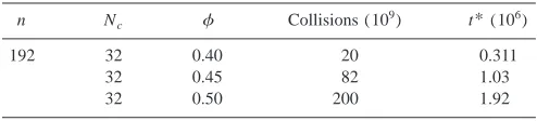
Table I summarizes the systems studied and includes the chain length, n, the number of chains, Nc, the volume
frac-tion,, the number of collisions, and the total times sampled during the production phases of the simulations. The simula-tion times are presented throughout the paper in terms of TABLE I. Size and length of the simulated systems.a
n Nc Collisions (109) t*(106)
192 32 0.40 20 0.311
32 0.45 82 1.03
32 0.50 200 1.92
a
reduced units, t*⫽(kBT/m2)1/2t, where kB is the Boltz-mann constant, T is the temperature, and m is the mass of a segment. All simulations were performed at a reduced tem-perature of kBT⫽1.0 and a mass of m⫽1.0 for all segments.
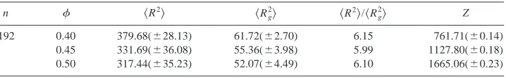
The static properties of the systems studied, including the mean squared end-to-end distance,
具
R2典
, the mean squared radius of gyration,具
Rg2典
, and the compressibility factor, Z, were monitored over the course of the simulations to confirm fluid equilibration. The mean squared end-to-end distance was calculated from具
R2典
⬅具
(r1⫺rn)2典
, where r1and rnare the coordinates of the first and last chain segments
and
具 典
denotes an ensemble average. The radius of gyration was calculated from具
Rg2典
⬅具
兺in⫽1(ri⫺rc.m.)2典
/n, where ri isthe position of segment i and rc.m.⫽(1/n)兺in⫽1riis the posi-tion of the chain center of mass. For a Gaussian chain, both the end-to-end distance and the radius of gyration should scale linearly with chain length so that the ratio
具
R2典
/具
Rg2
典
⬇6.21 The compressibility factor was calculated from the Clausius virial theorem: Z⫽n⫺(m兺collri j•⌬vi j)/ (3NckBTte), where ri jis the vector between segment centers at a collision, ⌬vi j is the velocity change for the colliding pair, Ncis the number of chains in the system, and teis theelapsed simulation time over which the sum is calculated. The results for the static properties,
具
R2典
,具
Rg 2
典
,具
R2典
/具
Rg 2典
, and Z are presented in Table II. The standard deviations in
具
R2典
,具
Rg2典
, and Z were determined from the average values for batches of the simulations containing 2 billion collisions each. The values obtained for具
R2典
/具
Rg2典
indicate that the chains used in this study are essentially Gaussian. The compressibility factor was found to be linear with chain length and consistent with the work of Zhou
et al.30Agreement between the static properties of the simu-lations and predicted behavior confirms the equilibration of the systems. With the confirmation of fluid equilibration, the production phases of the simulations were started in order to analyze the dynamic properties of the systems.
During the course of the simulations, the coordinates of all chain segments were stored so that they could be used to determine the dynamic properties. These coordinates were later analyzed to obtain the mean squared displacement re-sults presented in this paper.
III. CHAIN DYNAMIC PROPERTY CALCULATIONS
Microscopic information about polymer diffusion is ob-tained by analyzing the time dependence of chain and chain segment displacements. The atomic mean squared displace-ment, g(t), is the average squared distance a chain segment moves after a time, t, and is defined as
g共t兲⬅1 n
兺
i⫽1n
具
兩ri共t⫹t0兲⫺ri共t0兲兩2典
, 共3兲where ri(t) is the position of atom i at time t, the sum is
over all chain segments i, and
具 典
represents the ensemble average that is over all time origins t0 as well as over allmolecules. Equation共3兲provides the average mean squared displacement of all segments within the chains.
The average mean squared displacement for specific blocks of the chain can be obtained by restricting this calcu-lation to particular segments of the chain. For example, we have calculated the mean squared displacement for middle blocks of the chain and for end blocks of the chain. This was done by averaging over only those segments of interest. The middle block mean squared displacement averaged over k middle segments is calculated from
gmiddle共t兲⬅1
ki⫽n/2
兺
⫹1⫺k/2 n/2⫹k/2具
兩ri共t⫹t0兲⫺ri共t0兲兩2典
. 共4兲Likewise, the end block mean squared displacement aver-aged over k segments on each chain end is calculated from
gend共t兲⬅ 1
2k
冉
i兺
⫽1 k具
兩ri共t⫹t0兲⫺ri共t0兲兩2典
⫹
兺
i⫽n⫺(k⫺1) n
具
兩ri共t⫹t0兲⫺ri共t0兲兩2典
冊
. 共5兲Throughout the paper, the mean squared displacements are reported in reduced units by dividing by the diameter squared, 2.
The tube model19,3 predicts that an entangled chain ex-hibits four distinct types of motion as characterized by the scaling of the atomic mean squared displacement, g(t), with time. These four different types of motion are共1兲g⬃t1/2for
t⬍e, wheree is the entanglement time,共2兲g⬃t1/4 fore ⬍t⬍R, where R is the Rouse time,共3兲 g⬃t1/2 for R⬍t
⬍d, whered is the disengagement time, and共4兲g⬃t for t⬎d. In our previous work,17 the entanglement times were
estimated to be e⬇1800, 3000, and 4500 for the chains of length 192 at the volume fractions of ⫽0.40, 0.45, and 0.50. The Rouse times were estimated to be R⬇25 000, 67 000, and 100 000 at the volume fractions of ⫽0.40, 0.45, and 0.50. The disengagement times could not be deter-mined conclusively.
TABLE II. Static properties of the systems.a
n 具R2典 具
Rg
2典 具
R2典/具Rg
2典 Z
192 0.40 379.68(⫾28.13) 61.72(⫾2.70) 6.15 761.71(⫾0.14)
0.45 331.69(⫾36.08) 55.36(⫾3.98) 5.99 1127.80(⫾0.18)
0.50 317.44(⫾35.23) 52.07(⫾4.49) 6.10 1665.06(⫾0.23)
aThe mean squared end-to-end distance,具R2典, the mean squared radius of gyration,具R g
2典, the ratio of the sizes,
具R2典/具R g
2典, and the compressibility factor, Z, are reported. The chain sizes are reported in units of2. Values
IV. RESULTS AND DISCUSSION
In this section, we present and discuss the results from our molecular dynamics simulations. First, we investigate how the size of the block considered affects conclusions about the difference between the dynamics of end segments and middle segments of chain molecules. Next, we deter-mine which portion of the chain exhibits chain middle be-havior and which portions exhibit chain end bebe-havior. Fi-nally, we investigate the dynamics of segment relaxation at different positions along the chain to ascertain how the re-laxation propagates along the chain length.
A. Effect of block size on the difference between the dynamics of end and middle blocks
It is of interest to determine if large blocks are able to distinguish the behavior of chain ends from that of the chain middle. Experimental studies have been limited to consider-ing the dynamics of relatively large end and middle blocks containing between 25% and 50% of the chain segments.4 – 6 In contrast, simulation studies have investigated the dynam-ics of individual segments or small blocks containing up to 10 segments.7–17 In this study, we use both approaches to compare the mean squared displacement behavior of end and middle chain segments.
1. Triblock analysis
In this part of our study, each chain is divided into thirds and then the mean squared displacements are calculated by averaging over the chain end blocks, the chain middle block, and the whole chain. This analysis is similar to experiments performed on labeled triblock polymers made up of equal sized blocks.
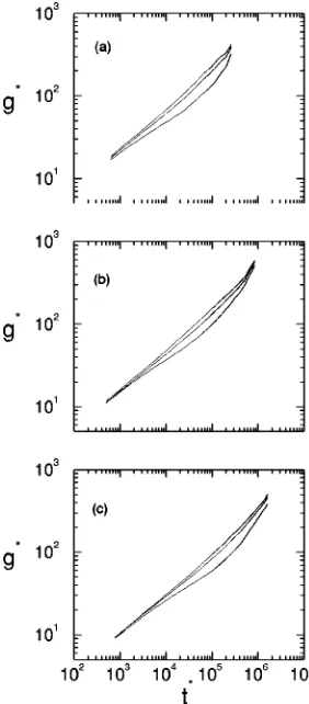
Figure 1 displays the mean squared displacements of the chain end sections, the chain middle section, and the whole chain for chains of length 192 at three different volume frac-tions, 共a兲 ⫽0.40, 共b兲 ⫽0.45, and共c兲 ⫽0.50. The top curve in each graph corresponds to the mean squared dis-placement of the end sections 共segments 1– 64 and 129– 192兲. The middle curve in each graph corresponds to the mean squared displacement averaged over all chain seg-ments. The bottom curve in each graph corresponds to the mean squared displacement of the middle section共segments 65–128兲.
For the triblock case, the mean squared displacements of the end blocks, the whole chain, and the middle blocks have similar values for each system. This is especially true at early times, t⭐e, when the three different mean squared
dis-placements are essentially identical. As time increases past e, a detectable difference is observed between the three
different mean squared displacements. The whole chain mean squared displacements are lower than the end block mean squared displacements but higher than the middle block mean squared displacements. This occurs because the end segments become more relaxed than the middle seg-ments and thus experience more mobility than the rest of the chain. At the same time, the middle segments remain con-fined and thus experience less mobility than the rest of the chain. As time increases further toward the longest times
reported, the three different mean squared displacements have similar values again as segments at all positions along the chain have relaxed.
The early-time simulation results are in qualitative agreement with the results from the NSE experiments of Ewen et al.4In their study of labeled triblock PDMS chains containing equal sized blocks, Ewen et al. found that the normalized coherent intermediate scattering function was es-sentially the same for the end and middle segments as it was for the whole chain. The NSE experiments were only able to access relatively short times, less than the Rouse time, which may not be long enough to reach the times when the greatest difference between the motion of the end and middle sec-tions occurs. Therefore, longer experimental times or smaller labeled sections may be needed to observe a distinct differ-ence between the behavior of the end and middle sections.
2. Small-block analysis
middle. These blocks of segments are small enough to con-centrate the analysis to specific parts of the chain but large enough to obtain good statistics.
Figure 2 displays the mean squared displacement aver-aged over the chain end sections, the chain middle section, and the whole chain for chains of length 192 at 共a兲 ⫽0.40,共b兲⫽0.45, and共c兲⫽0.50. As in the triblock case
共and as expected兲, the top curve is for the mean squared displacements averaged over the outer segments, the middle curve is for that averaged over all segments, and the bottom curve is for that averaged over the middle segments. In the small block case, the end sections include segments 1–5 and 188 –192, and the middle sections include segments 92–101. For the small-block case, the mean squared displace-ments of the end blocks are significantly different from those of the whole chain and those of the middle blocks for all of the systems studied. At the earliest times shown, t⭐e, the
mean squared displacements averaged over the middle sec-tions are essentially the same as those averaged over the whole chain, while those averaged over the end sections are much larger. This indicates that the endmost segments are more mobile than the rest of the chain. As time increases past e, the mean squared displacement curves of the middle
blocks separate from those of the whole chain, indicating decreased mobility and increased confinement of the middle sections. At longer times, all of the mean squared
displace-ment curves approach each other as all of the segdisplace-ments of the chains relax.
There is a larger separation between the different mean squared displacement curves in the small-block case than there was in the triblock case. The difference between the mean squared displacements of the end and middle blocks is much greater here than it was for the triblock case.
3. Comparison between the triblock analysis and the small-block analysis
The differences between the results from the equal sized triblock case and those from the small-block case can be seen more clearly by comparing the mean squared displacement results obtained for the end and middle chain sections from the two methods on the same graph.
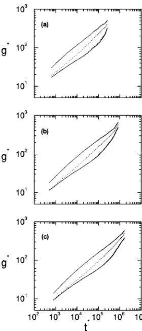
Figure 3 displays the mean squared displacement results for the end and middle blocks from both the triblock and small-block cases for chains of length 192 at 共a兲 ⫽0.40,
共b兲 ⫽0.45, and 共c兲 ⫽0.50. The results for the triblock case are represented by dotted lines, and the results for the small-block case are represented by solid lines. In each graph, the top curve is the end section mean squared dis-placement for the small-block case. The second curve from the top is always the end section mean squared displacement FIG. 2. Reduced mean squared displacement vs reduced time for the chains
of length 192 at共a兲⫽0.40,共b兲⫽0.45, and共c兲⫽0.50. Included, from top to bottom, are the mean squared displacements of the end blocks, the whole chain, and the middle block for the small-block case.
for the triblock case. The bottom two curves are always the middle section mean squared displacements for the triblock and small-block cases.
There is a large difference between the end section mean squared displacements from the triblock and small-block cases over all of the times studied, but the difference is smaller at long times. The middle section mean squared dis-placements are essentially the same in the triblock case as in the small-block case over all times. This indicates that a larger portion of the chain has middle section behavior than has end section behavior. Therefore, small blocks must be used to probe the end section behavior, but larger blocks can be used to probe the middle section behavior.
The ratio of the end block to middle block mean squared displacement was calculated for the different cases. This ra-tio can be used to determine the difference in the mobility of the chain ends and the chain middle and to compare the ability of the triblock and small-block studies to capture this difference. The ratio was also calculated for the end segment on each chain end and the two middle segments to compare the results for the triblock and small-block cases to the lim-iting case, which is expected to reveal the actual behavior of the middle and end segments. The maximum value can also be compared to the Rouse model and reptation predictions, as was done by Kreer et al.,8 to determine which model is better able to capture the dynamics of the different chain sections.
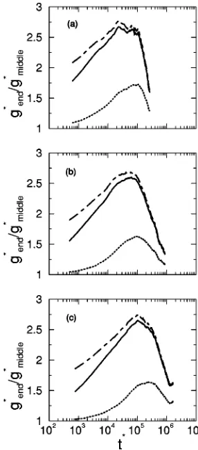
Figure 4 displays the ratio of the end block mean squared displacement to the middle block mean squared dis-placement for both the triblock and small-block cases for chains of length 192 at 共a兲 ⫽0.40, 共b兲 ⫽0.45, and 共c兲 ⫽0.50. Also included for comparison is the ratio of the end segment共segments 1 and 192兲to middle segment共segments 96 and 97兲mean squared displacement. The top共dot-dashed兲 curve in each graph is for the limiting case, the middle
共solid兲curve is for the small-block case, and the bottom共 dot-ted兲curve is for the triblock case.
The ratio of the end block mean squared displacement to the middle-block mean squared displacement provides a good measure of the difference between the dynamics of the different size blocks considered. The small-block case cap-tures the difference in mobility between the chain end seg-ments and the chain middle segseg-ments much better than the triblock case. The ratio for the small-block case is very close to the limiting case; whereas, the ratio for the triblock case is much smaller and does not change as much over time. Small blocks, or the limiting segments, are needed to compare the maximum in this ratio to the theoretically predicted value, because the maximum in the triblock case is dramatically smaller than in the limiting case. For chains of length 192, the maximum in the ratio for the triblock case is mately 1.6 –1.7, whereas for the other cases it is approxi-mately 2.6 –2.8. The maximum value for the triblock case is less than the Rouse prediction of 2; the maximum values for the other cases are greater than the Rouse prediction but less than the reptation prediction of 4&共5.656兲. The large blocks in the triblock case are too large to capture the true depen-dence of segment position along the chain on the dynamic behavior, and thus smaller sections should be used.
B. Portion of segments exhibiting chain end and chain middle behavior
In this section we determine what portion of the chain exhibits middle behavior and what portion exhibits end be-havior. The aim is to determine what size blocks are suffi-cient to capture the middle section and end section behavior, as measured by the mean squared displacements.
1. Portion of segments exhibiting chain middle behavior
The mean squared displacements of different sized blocks of middle segments were analyzed to determine how large the middle blocks can be and still display primarily middle section behavior.
Figure 5 displays the mean squared displacements of blocks of middle segments of different sizes as a function of reduced time for chains of length 192 at 共a兲 ⫽0.40, 共b兲 ⫽0.45, and共c兲⫽0.50. The middle block sizes are 2, 10, 64, 96, 128, and 172 segments. Most of these mean squared displacement curves are the same as that for the smallest middle block containing two segments 共bottom curve兲. The ability of the different sized middle blocks to mimic the be-havior of the middle segments depends on the time range of interest. At the early times, t⭐e, there is no detectable
different sized middle blocks. During intermediate times, t
⬇R, the mean squared displacements of the three largest
middle blocks studied, containing 96, 128, and 172 seg-ments, are larger than those of the smaller middle blocks. This suggests that the segments in these larger blocks that are closer to the ends have started relaxing by this time. At longer times, the mean squared displacements of the differ-ent sized blocks approach the same curve again.
From the mean squared displacement curves of the dif-ferent sized middle blocks, it appears that the middle blocks containing 2, 10, and 64 segments provide similar behavior. The mean squared displacements of the larger middle blocks
共96, 128, and 172 segments兲 exhibit some deviation from that of the middle segments during the intermediate times aroundR. To determine the extent of the deviation between the different sized middle blocks, the fractional difference between the mean squared displacement of each sized block and that of the smallest block containing two segments was calculated and analyzed.
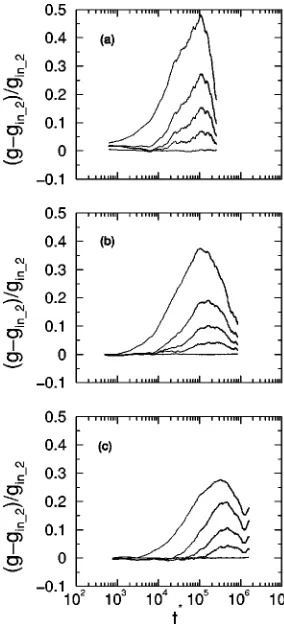
Figure 6 displays the fractional difference between the mean squared displacements of the different sized middle blocks 共10, 64, 96, 128, and 172 segments兲 and that of the reference middle block containing two segments as a func-tion of reduced time for chains of length 192 at 共a兲 ⫽0.40, 共b兲⫽0.45, and共c兲⫽0.50. The curves from top to bottom are for blocks containing 172, 128, 96, 64, and 10
segments. Over the whole time range, the fractional differ-ence for the block containing 10 segments is approximately zero. At early times, the fractional differences for the other sized blocks is small, and some have smaller mean squared displacements than the two-segment reference block. The reference block should have the smallest mean squared dis-placement at all times. Although this is not observed, the most negative fractional difference, ⫺0.01, is probably not significantly different than 0. As time increases, the frac-tional differences for the larger blocks increase. The maxi-mum value in the fractional difference provides a measure of the different sized middle blocks’ ability to mimic the behav-ior of the middle segments.
Table III lists the maximum fractional difference be-tween the mean squared displacement of the different sized middle blocks and that of the reference middle block con-taining two segments. The values are largest for the chains at the smallest volume fraction, ⫽0.40, and similar for the chains at the other two volume fractions,⫽0.45 and 0.50. This indicates that the chains are more confined, and more segments exhibit middle behavior at the larger volume tions. For any given volume fraction, the maximum frac-tional difference increases with increasing middle block size as expected. The maximum fractional difference is less than 0.11 for the middle blocks containing 10 segments and 64 segments at all volume fractions and for the middle blocks FIG. 5. Reduced mean squared displacement of middle blocks vs reduced
time for chains of length 192 at 共a兲 ⫽0.40, 共b兲 ⫽0.45, and 共c兲
⫽0.50. Included are the mean squared displacements for middle blocks containing 172, 128, 96, 64, 10, and 2 segments, from top to bottom.
FIG. 6. Fractional difference between the mean squared displacement of different sized middle blocks and that of the reference middle block con-taining two segments vs reduced time for chains of length 192 at 共a兲
containing 96 segments at the higher volume fractions, ⫽0.45 and 0.50. This indicates that more of the chain is confined, and thus more segments exhibit middle behavior at the higher volume fractions.
2. Portion of segments exhibiting chain end behavior
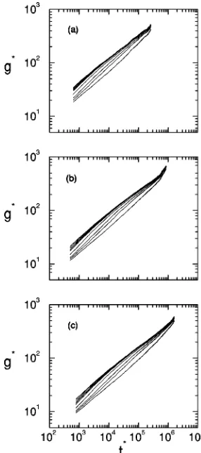
The mean squared displacements of different sized blocks of end segments were analyzed to determine how large the end blocks can be and still display primarily end section behavior. Figure 7 displays the mean squared dis-placements of blocks of end segments of different sizes as a function of reduced time for chains of length 192 at 共a兲
⫽0.40, 共b兲 ⫽0.45, and 共c兲⫽0.50. The end block sizes are 1, 2, 3, 4, 5, 10, 20, 32, and 64 segments共on each side of the chain兲, from top to bottom. Most of the mean squared displacement curves are different than that of the smallest end block containing one segment. The ability of the differ-ent sized end blocks to mimic the behavior of the end seg-ments depends on the time range of interest. At the early times, the largest difference between the mean squared dis-placements of the different sized end blocks is observed. As time increases, the mean squared displacements of the differ-ent sized blocks approach the same curve.
From the mean squared displacement curves for the dif-ferent sized end blocks, it appears that very small end blocks are needed to minimize the deviation between the end block behavior and that of the endmost segments. To determine the extent of the deviation between the different sized end blocks, the fractional difference between the mean squared displacement of each sized block and that of the smallest block containing one segment was calculated and analyzed.
Figure 8 displays the fractional difference between the mean squared displacement of different sized end blocks and that of the reference end block containing one segment as a function of reduced time for chains of length 192 at 共a兲 ⫽0.40,共b兲⫽0.45, and共c兲⫽0.50. The curves, from bot-TABLE III. Maximum fractional difference for the different sized middle
blocks.a
Number of segments
10 64 96 128 172
0.40 0.0051 0.0706 0.1545 0.2734 0.4823
0.45 0.0026 0.0437 0.1030 0.1924 0.3754
0.50 0.0038 0.0448 0.1076 0.1987 0.2774
a
The maximum fractional differences between the mean squared displace-ment of different sized middle blocks and that of the two middle segdisplace-ments are reported. The different sized middle blocks include 10, 64, 96, 128, and 172 segments in the chain middle.
FIG. 7. Reduced mean squared displacement of end blocks vs reduced time for chains of length 192 at 共a兲 ⫽0.40, 共b兲⫽0.45, and共c兲 ⫽0.50. Included are the mean squared displacements for end blocks containing 1, 2, 3, 4, 5, 10, 20, 32, and 64 segments共on each side of the chain兲, from top to bottom.
FIG. 8. Fractional difference between the mean squared displacement of different sized end blocks and that of the reference end block containing one segment共on each chain end兲vs reduced time for the chains of length 192 at
共a兲 ⫽0.40, 共b兲 ⫽0.45, and 共c兲 ⫽0.50. Included are the fractional differences for end blocks containing 2, 3, 4, 5, 10, 20, 32, and 64 segments
tom to top, are for the fractional differences for the end blocks containing 2, 3, 4, 5, 10, 20, 32, and 64 segments on each chain end. None of the blocks exhibit a fractional dif-ference of zero when compared to the end segments. At early times, t⭐e, the fractional differences for the different sized
blocks are large. All of the different sized end blocks, except the two largest 共those containing 32 and 64 segments兲, ex-hibit their maximum fractional difference at the initial time shown. The two largest end blocks reach their maximum fractional difference at times around e. As time increases
further, the fractional differences of all of the different sized blocks decrease. The maximum value in the fractional differ-ence provides a measure of the different sized end blocks’ ability to mimic the behavior of the end segments.
Table IV lists the maximum fractional difference be-tween the mean squared displacement of the different sized end blocks and that of the reference end block containing one segment. The values are largest for the chains at the largest volume fraction of⫽0.50. This indicates that more of the chain is confined, and thus fewer segments exhibit end behavior at larger volume fraction. For any given volume fraction, the maximum fractional difference increases with increasing end block size as expected. The maximum frac-tional difference is only less than 0.1 for the end blocks containing two segments at all volume fractions and for the end block containing three segments at the lowest volume fraction of⫽0.40.
C. Dynamics of segment relaxation along the chain
In this section, we study the dynamics of segment relax-ation along the chain. The aim is to determine how segment relaxation propagates along the length of the chain with in-creasing time. This information is helpful for determining the mechanism of chain relaxation and, thus, provides informa-tion about entanglement relaxainforma-tion.
1. Mean squared displacements of small blocks of segments at various positions along the chain
The mean squared displacements of small blocks of seg-ments at various positions along the chain were analyzed to determine how segment position affects the time when en-tanglement relaxation occurs and hence obtain information about the mechanism of entanglement relaxation and release. The tube model predicts that tube relaxation starts at the chain ends and progresses along the chain toward the chain middle where final relaxation occurs. As this relaxation oc-curs, the ends of the chain escape the tube and become part of the two minor chains共one on each chain end兲. The minor
chains are the end portions of the chain which have relaxed. The minor chain length increases with time as the relaxation progresses along the chain length. When the mean squared displacement of a particular block increases more than that of the middle block, the segments in that block have relaxed and become part of a minor chain. We use the time when this relaxation occurs to determine how the minor chain length increases with increasing time.
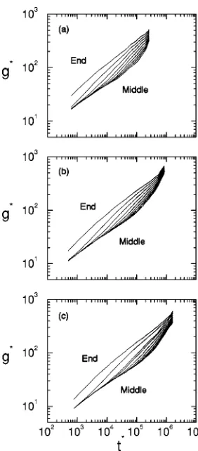
Figure 9 displays the mean squared displacements of blocks of segments at various positions along the chain as a function of reduced time for chains of length 192 at 共a兲 ⫽0.40, 共b兲 ⫽0.45, and 共c兲 ⫽0.50. The mean squared displacement curves for nine different blocks of segments at TABLE IV. Maximum fractional difference for the different sized end blocks.a
Number of segments共on each side兲
2 3 4 5 10 20 32 64
0.40 0.0389 0.0755 0.1098 0.1416 0.2615 0.3721 0.4232 0.4799
0.45 0.0547 0.1035 0.1464 0.1836 0.3014 0.3854 0.4278 0.4905
0.50 0.0629 0.1180 0.1649 0.2042 0.3181 0.3927 0.4319 0.4965
a
The maximum fractional differences between the mean squared displacements of different sized end blocks and that of the segment on each chain end are reported. The different sized end blocks include 2, 3, 4, 5, 10, 20, 32, and 64 segments on each chain end.
various positions along the chain are included. The top curve is for the 5 outer segments 共segments 1–5 and 188 –192兲. The next seven curves are for blocks of segments at interme-diate positions along the chain and include the following groups of 10 segments: segments 11–15 and 178 –182, 21–25 and 168 –172, 31–35 and 158 –162, 41– 45 and 148 – 152, 51–55 and 138 –142, 61– 65 and 128 –132, and 71–75 and 118 –122. The bottom curve is for the 10 inner segments
共segments 92–101兲.
At the earliest times shown in Fig. 9, all of the blocks, except the one containing the endmost segments共top curve兲, have moved approximately the same distance. This indicates that chain connectivity is the dominant factor during this time range, as the tube model dictates. The end block is able to move more than the other blocks because the end seg-ments are bound on only one side while the other segseg-ments are bound on both sides. As time increases, the various mean squared displacements begin to fan out as intermediate blocks containing segments near the chain ends experience more relaxation than the inner segments, as indicated by the increase in slope of the mean squared displacement curve. First, the block that includes segments 11–15 and 178 –182
共second curve from top兲begins to relax. This relaxation then progresses to the next block共segments 21–25 and 168 –172兲 along the chain closer to the chain middle and continues with the next sections in order toward the chain middle. This in-dicates that the initial relaxation of entanglements occurs near the chain ends and progresses toward the chain middle with time, as the tube model predicts. The time when a block relaxes is used to determine the minor chain length as a function of time as is explained below.
2. Relaxation time of blocks at various positions along the chain
When the mean squared displacement of a particular block increases beyond that of the middle block, the seg-ments in that block have relaxed and become part of a minor chain. At the time when a block has relaxed, the minor chain length has increased to include the segments in that block. Therefore, the times when blocks at various positions relax are used to determine how the minor chain length increases with time. The time when the relaxation of a block occurs was determined by comparing the mean squared displace-ment of that block to that of the middle block.
Three different methods were used to obtain an average value for each block’s relaxation time. These values were then used in the minor chain investigation. First, the relax-ation time of a block was estimated as the time when its mean squared displacement curve experiences a large in-crease in slope compared to that of the middle block, causing its mean squared displacement to increase above that of the middle block. Next, the actual data points were included with the mean squared displacement curves, and the relaxation time of a block was estimated as the time of the data point closest to the time when the block’s mean squared displace-ment curve experienced a large increase in comparison to that of the middle block. Finally, the fractional difference between the mean squared displacement of each block and that of the middle block was calculated and plotted versus
time on a logarithmic scale. The relaxation time was esti-mated as the time of the data point at which the fractional difference began to increase. The three relaxation times for each block along the chain were averaged to obtain the
共arithmetic mean兲 relaxation time for each block. For each block along the chain, the number of segments in the minor chain was estimated based on the average position of the segments in the block. These estimated relaxation times and minor chain lengths were used to compare the simulation results to the minor chain reptation model predictions, as discussed below.
3. Minor chain length as a function of time
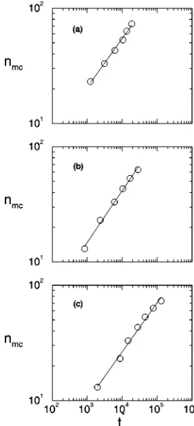
The behavior of the estimated minor chain lengths as a function of time was determined in order to obtain more information about entanglement relaxation and to compare the simulation results to theoretical predictions. The minor chain reptation model predicts that the number of segments in the minor chain, nmc, exhibits power law scaling with time so that nmc⬃t0.5.31,32We obtain a power law fit to the estimated minor chain lengths versus time to determine how well our simulation results fit this trend.
age segment positions of the small blocks, and the estimated times are the average times when those blocks became more relaxed than the middle blocks as determined from the mean squared displacements. The lines correspond to a power law fit to the estimated data points.
The estimated minor chain lengths versus time of all of the systems essentially fall on a straight line in the log–log plot, indicating that the minor chain length follows a power law with time. The power law fits (nmc⬃tx) to the data for the different systems provide similar exponents: x⬇0.42 ⫾0.03, 0.45⫾0.03, and 0.42⫾0.03, at ⫽0.40, 0.45, and 0.50. These exponents are somewhat less than the predicted value of 0.5. The relaxation of chain segments progresses from the chain ends toward the chain middle, and the minor chain lengths exhibit power law behavior with time. How-ever, the lower than predicted exponents suggest that the relaxation of the segments along the chain progresses some-what more slowly than the minor chain reptation model pre-dicts.
V. CONCLUSIONS
In this study, discontinuous molecular dynamics simula-tions were performed to investigate how a segment’s position along the chain affects its mean squared displacement. First, we studied how the size of the blocks of segments consid-ered affects the difference between the dynamics of end and middle segments. Then, we determined what portion of the chain exhibits chain middle behavior and what portion ex-hibits chain end behavior. Finally, we investigated the dy-namics of segment relaxation along the chain to ascertain how the relaxation propagates along the chain.
We studied how the size of the block considered affects conclusions about the difference between the dynamics of end and middle segments of chain molecules. The aim was to determine if large blocks, like those used during experi-ments, are able to distinguish the dynamics of chain ends from that of the chain middle. First, we analyzed the mean squared displacements of chain end segments, chain middle segments, and the whole chain for triblock chains. For the triblock case, we found that the mean squared displacements of the end blocks, the middle blocks, and the whole chain exhibit similar values, and that the greatest difference oc-curred during the intermediate times sampled. Next we ana-lyzed the mean squared displacements of chain end seg-ments, chain middle segseg-ments, and the whole chain for the case where just ten segments were used to represent the chain end or the chain middle. For the small-block case, we found that there was a larger difference between the three mean squared displacement curves than there was for the triblock case. Finally, we compared the results from the tri-block and small-tri-block cases directly. There was a large dif-ference between the end block mean squared displacements from the triblock and small-block cases. However, the middle-block mean squared displacements were essentially the same in the two cases. The ratio of the end block mean squared displacement to the middle-block mean squared dis-placement was calculated for the different cases to determine the difference between the dynamics of the end and middle
blocks. It was found that the small blocks were needed to capture the difference between the end and middle-block mean squared displacements.
The study on the dynamics of different sized blocks was extended to include other size blocks to determine what por-tion of the chain exhibited chain middle behavior and what portion exhibited chain end behavior. The aim was to deter-mine what size blocks are sufficient for studying the middle section or end section mean squared displacements. From the mean squared displacements of different sized middle blocks, it was found that very large middle blocks provide similar results to very small middle blocks. This indicates that a large portion of the chain exhibits chain middle behav-ior. On the other hand, the mean squared displacements of different sized end blocks indicated that small end blocks are needed to obtain end segment behavior. Therefore, a small portion of the chain exhibits chain end behavior.
The dynamics of segment relaxation along the chain were studied to determine how segment relaxation propa-gates along the length of the chain with increasing time. First, the mean squared displacement versus time was ana-lyzed for small blocks of segments at various positions along the chain. The relaxation of these blocks started at the chain ends and progressed toward the chain middle with time, as the tube model predicts. The time when the relaxation of a block occurred was estimated by determining when the block’s mean squared displacement increased above that of the middle block. These estimated relaxation times repre-sented the time at which the minor chain included segments along the chain up to the middle of that block. The minor chain length versus time exhibited the power law behavior
nmc⬃tx, where x⬇0.42⫾0.03, 0.45⫾0.03, and 0.42⫾0.03 at ⫽0.40, 0.45, and 0.50. This time dependence was slightly lower than the value x⫽0.5 predicted by the minor chain reptation model.
ACKNOWLEDGMENTS
We would like to thank J. van Zanten for helpful discus-sions. This work was supported by a National Science Foun-dation Graduate Research Fellowship, a DuPont Graduate Fellowship, an Eastman Graduate Fellowship, and the Office of Energy Research, Basic Sciences, Chemical Science Divi-sion of the U.S. Department of Energy under Contract No. DE-FG02-97-ER14771. Acknowledgment is made to the Do-nors of the Petroleum Research Fund administered by the American Chemical Society for partial support of this work. We thank the North Carolina Supercomputing Center for grants of computing time and file storage space.
1P. E. Rouse, J. Chem. Phys. 21, 1272共1953兲. 2P. G. de Gennes, J. Chem. Phys. 55, 572共1971兲.
3M. Doi and S. F. Edwards, The Theory of Polymer Dynamics共Oxford
University Press, Oxford, 1986兲.
4
B. Ewen, D. Richter, and B. Farago, Acta Polym. 45, 143共1994兲.
5K. Welp, R. Wool, S. Satija, S. Pispas, and J. Mays, Macromolecules 31,
4915共1998兲.
6K. Welp, R. Wool, G. Agrawal, S. Satija, S. Pispas, and J. Mays,
Macro-molecules 32, 5127共1999兲.
7
8T. Kreer, J. Baschnagel, M. Muller, and K. Binder, Macromolecules 34,
1105共2001兲.
9J. Skolnick and A. Kolinski, Adv. Chem. Phys. 78, 223共1990兲. 10
K. Kremer and G. S. Grest, J. Chem. Phys. 92, 5057共1990兲.
11B. Dunweg, G. S. Grest, and K. Kremer, in Numerical Methods for Poly-meric Systems, edited by S. G. Whittington共Springer-Verlag, New York, 1998兲.
12M. Pu¨tz, K. Kremer, and G. S. Grest, Europhys. Lett. 49, 735共2000兲. 13
S. W. Smith, C. K. Hall, and B. D. Freeman, Phys. Rev. Lett. 75, 1316 共1995兲.
14S. W. Smith, C. K. Hall, and B. D. Freeman, J. Chem. Phys. 104, 5616
共1996兲.
15
S. W. Smith, C. K. Hall, B. D. Freeman, and J. A. McCormick, in Nu-merical Methods for Polymeric Systems, edited by S. G. Whittington
共Springer-Verlag, New York, 1998兲.
16A. Kolinski, J. Skolnick, and R. Yaris, J. Chem. Phys. 86, 1567共1987兲. 17J. A. McCormick, C. K. Hall, and S. A. Khan, Macromolecules共to be
published兲.
18K. S. Schweizer, J. Chem. Phys. 91, 5822共1989兲.
19M. Doi and S. F. Edwards, J. Chem. Soc., Faraday Trans. 2 74, 1789
共1978兲.
20S. W. Smith, C. K. Hall, and B. D. Freeman, J. Comput. Phys. 134, 16
共1997兲.
21P. J. Flory, Statistical Mechanics of Chain Molecules共Interscience, New
York, 1969兲.
22D. C. Rapaport, J. Phys. A 11, L213共1978兲.
23A. Bellemans, J. Orban, and D. V. Belle, Mol. Phys. 39, 781共1980兲. 24B. J. Alder and T. E. Wainwright, in Symposium on Transport Processes in
Statistical Mechanics, edited by I. Prigogine 共Interscience, New York, 1956兲.
25B. J. Alder and T. E. Wainwright, J. Chem. Phys. 31, 459共1959兲. 26J. M. Haile, Molecular Dynamics Simulation: Elementary Methods
共Wiley, New York, 1992兲.
27
M. P. Allen and D. J. Tildesley, Computer Simulation of Liquids共 Claren-don, Oxford, 1987兲.
28D. C. Rapaport, J. Comput. Phys. 34, 184共1980兲.
29J. J. Erpenbeck and W. W. Wood, in Modern Theoretical Chemistry, edited
by B. J. Berne共Plenum, New York, 1977兲.
30
Y. Zhou, S. W. Smith, and C. K. Hall, Mol. Phys. 86, 1157共1995兲.
31Y. H. Kim and R. P. Wool, Macromolecules 16, 115共1983兲.
32R. P. Wool, Polymer Interfaces; Structure and Strength共Hanser, Munich,