HELLER, MARTIN ANDREW. Robust Minimum Density Estimators and Stochastic Resonance for Classification Algorithms. (Under the direction of Dr. Kazufumi Ito).
This dissertation is devoted to robust statistical methods. Part one deals with robust esti-mation methods. Specifically, the Robust Minimum Density Estimator (RMDE) is developed along with a Bayesian methodology incorporating the benefits of the RMDE. The second part considers robust methods for classification algorithms. This includes a method to differentiate textures along with a method to boost the fidelity of general classification algorithms when classes have limited information.
The class of RMDE’s are a subset of Minimum Density Estimators (MDE). RMDE’s treat a sample as a single observation of a random distribution function. The deviance of a small number of observations does not change the general shape of the random distribution function. As the RMDE finds estimators based on the general shape of the random distribution function, the RMDE has a great resistance to outliers. Asymptotic results of the RMDE are presented including consistency and bounds on the variance function.
Once the asymptotic results are presented, the generality of the estimator is presented. Techniques of parameter estimation specific to the RMDE are developed. Simulations are presented to compare the RMDE estimator with standard estimation methods with and without the addition of outliers. The estimation methods are then extended to regression problems which do not differ for linear and nonlinear regression problems. The same method may also be used for regression with heteroscedasticity.
by
Martin A. Heller
A dissertation submitted to the Graduate Faculty of North Carolina State University
in partial fullfillment of the requirements for the Degree of
Doctor of Philosophy
Applied Mathematics
Raleigh, North Carolina 2009
APPROVED BY:
Dr. Charles Smith Dr. Ralph Smith
Dr. Kazufumi Ito Dr. Min Kang
DEDICATION
I dedicate this dissertation to my wife Fang-Shu Ou for her love and support; my parents Leonard and Marilyn Heller for their unyielding dedication; Professor Kosorok for inspiration; and my
BIOGRAPHY
Martin A Heller was born in St Louis, Missouri on April 12th, 1978. Three moves later he ar-rived in Stanwood, a small town about 50 miles north of Seattle, Washington. He dropped out of Stanwood High School at the age of 16 and got his GED. After terminating his high school tenure, he took several classes at Skagit Valley College, while independently studying various science and mathematics topics.
Martin began his studies at Western Washington University as a full time student in the winter of 1999. After three and a half years Martin graduated with a Bachelor of Science in Ap-plied Mathematics specializing in Operations Research and Engineering Mathematics, along with a Bachelor of Arts in Chemistry in June of 2002. Lacking a strong memory he decided to continue his studies in the mathematical sciences rather than chemistry. To do so he enrolled for a master’s degree in statistics at the University of Wisconsin-Madison. Two years of study lead to the Master of Science in Statistics in May of 2004.
While a student Martin met his future wife, Fang-Shu Ou, in the office next to his in the statistics department. As she was one year behind him in school he took a job as a programmer at Epic Systems while she completed her degree. Once she completed her degree, they moved to Raleigh so Martin could work on a PhD degree. They were finally married in October of 2005.
TABLE OF CONTENTS
LIST OF TABLES . . . vi
LIST OF FIGURES . . . vii
I Robust statistical methods 1 1 Robust minimum density estimators . . . 4
1.1 Asymptotic consistency of the RMDE . . . 6
1.2 Asymptotic variances and distributions of the RMDE . . . 8
1.2.1 Convergence of the first and second derivatives for φn(θ) at the optimal solutionθ0 . . . 10
1.2.2 Variance whenP(F= Fθ) =0. . . 21
1.2.3 Variance whenP(F= Fθ) =1. . . 25
1.3 Numerical methods for evaluation of theφn,φ, and optimization overΘ . . . 29
1.4 Simulations . . . 30
1.4.1 Other estimation methods for comparison . . . 32
1.4.2 Results of various simulations . . . 36
1.4.3 A comparison of the topologies imposed by the asymptotic MLE and RMDE objective functions . . . 39
1.4.4 Further simulation with outliers . . . 40
1.5 RMDE for regression . . . 42
1.5.1 Simulation of regression for comparison of ordinary least squares and RMDE regression . . . 45
1.6 Discussion . . . 46
2 Posterior distributions using the robust minimum density estimator . . . 49
2.1 The RMDE posterior distribution . . . 51
2.2 Simulations . . . 54
2.2.1 Simulations of the posterior distribution . . . 55
2.2.2 Point estimators using the simulated distributions . . . 56
2.3 Other Bayesian techniques . . . 59
2.3.1 Sampling from the RMDE posterior distribution . . . 59
2.3.2 Sequences of posterior distributions . . . 59
2.3.3 Comparison of credible regions and confidence intervals . . . 60
II Classification 66
3 Classification . . . 67
3.0.1 Mathematical formulation of the classification problem . . . 69
3.1 Evaluation of classifiers . . . 71
3.1.1 False negatives and false positives . . . 73
3.2 Feature extraction . . . 74
3.3 Classification algorithms . . . 74
3.3.1 Bayesian classifier . . . 76
3.3.2 Bayesian classifiers using estimated densities . . . 77
3.3.3 k-Nearest neighbor . . . 82
3.3.4 Binary tree classifier . . . 82
3.3.5 Iterative partial least squares discriminant analysis . . . 86
4 Classification of textures . . . 89
4.1 Models for uniform random fields . . . 91
4.1.1 Simultaneous autoregressive model and the vector autoregressive model . . 91
4.2 Theory . . . 93
4.2.1 Topological equivalence of the first-order autoregressive and first-order si-multaneous autoregressive models for radially symmetric random fields . . 94
4.3 Simulations using gaussian random fields . . . 96
4.3.1 Robustness of the VAR algorithm . . . 98
4.4 VAR classifier accuracy for real texture data . . . 98
4.5 Discussion . . . 100
5 Stochastic resonance . . . 101
5.1 Simulation . . . 103
5.2 Informal reasoning . . . 106
6 Stochastic resonance for yellow cake . . . 108
6.1 Data sets . . . 109
6.1.1 Comparison of LLNL002 and REF datasets . . . 110
6.2 Training the classifiers using REF . . . 111
6.2.1 Training the classifiers with stochastic resonance . . . 112
6.2.2 Focus on country and region . . . 114
6.2.3 Reduction of the maximum sample size . . . 115
6.3 Results of analysis of LLNL002 . . . 115
6.4 Correction for change in mine density . . . 116
6.5 Discussion . . . 117
Bibliography . . . 118
LIST OF TABLES
Table 2.1 Conjugate priors . . . 54
Table 4.1 Accuracy of classifier using the VAR features to separate textures . . . 99
Table 6.1 Distribution of Mines . . . 109
Table 6.2 Measurement differences between REF and LLNL002 . . . 110
Table 6.3 Small sample comparisons . . . 115
Table 6.4 Table displaying the results of predicting the class of the unknowns using only data from the reference set. . . 116
Table A.1 Fitting of classifiers without correction for the class distribution . . . 122
Table A.2 Fitting of classifiers without distribution correction for classification of country . . . 123
Table A.3 Fitting of classifiers without distribution correction for classification of continent . . . 123
Table A.4 Confusion matrix for CART classifier with equal weights for each classes . . . 127
LIST OF FIGURES
Figure 1.1 φnand ∂φ∂θn(θ) whenP(F=Fθ) =1 . . . 26
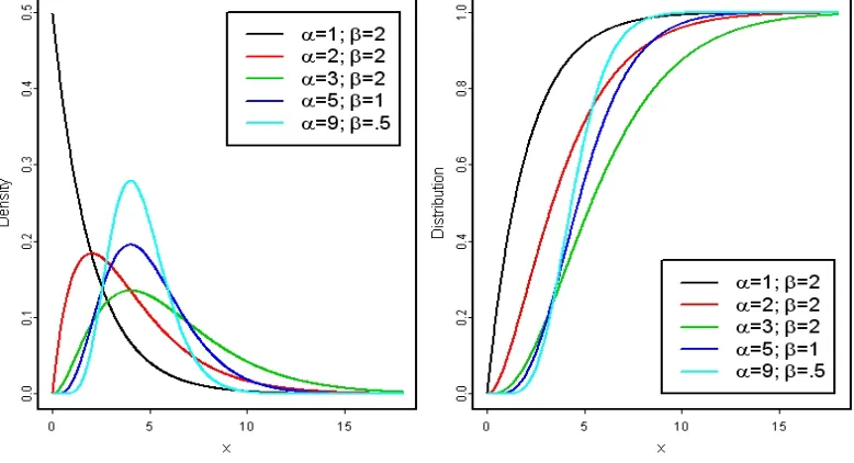
Figure 1.2 Gamma density and distribution functions . . . 31
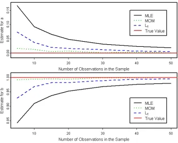
Figure 1.3 Estimation of the shapeα=2parameter inΓ(2, 2). . . 36
Figure 1.4 Estimation of the shapeβ=2parameter inΓ(2, 2). . . 37
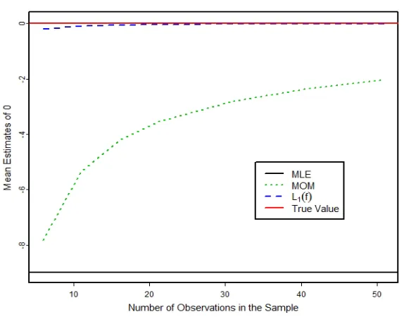
Figure 1.5 Estimation ofa=0andb=1of the standard uniform distribution. . . 38
Figure 1.6 Estimation of the lower bound ofU(0, 1)with junk data. . . 39
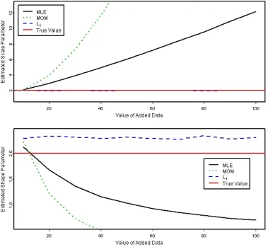
Figure 1.7 Estimation ofΓ(2, 2)vs value of biased point. . . 41
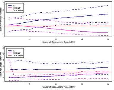
Figure 1.8 Hellinger and RMDE estimation ofΓ(2, 2)vs number of bad points. . . 43
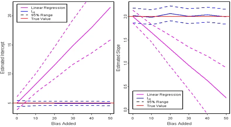
Figure 1.9 Comparison of regular linear regression and RMDE regression. . . 44
Figure 1.10 Initial distributions leading to different RMDE estimators . . . 47
Figure 2.1 Distribution of theL1cost function . . . 52
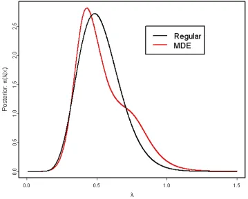
Figure 2.2 Example of a posterior distribution . . . 55
Figure 2.3 Posterior point estimators vs sample size for the gamma distribution . . . 57
Figure 2.4 Effects of bias on point estimators of the exponential distribution . . . 58
Figure 2.5 The effects of bias on point estimators of the Pareto distribution . . . 63
Figure 2.6 The effects of bias on point estimators of the normal distribution . . . 64
Figure 2.7 The effects of bias on point estimators of the Pareto distribution with an improper prior . . . 65
Figure 3.1 Diagram depicting the general classification algorithm . . . 70
Figure 3.3 A simple binary tree classifier. . . 83
Figure 4.1 Examples of textures . . . 90
Figure 4.2 Simulated 200-by-100 data set forγ=1andθ=.05. . . 97
Figure 4.3 Simulated 200-by-200 data set forγ=1andθ=.05. . . 98
Figure 4.4 Accuracy of VAR classification for a radially symmetric exponential covariance function withγ=1. . . 99
Figure 4.5 Test for robustness of the VAR algorithm for deviance from the tested model. . . 100
Figure 5.1 Stochastic resonance for a bistable system . . . 102
Figure 5.2 Bayes classification for 2 classes in<. . . 104
Figure 5.3 The effects of stochastic resonance on one step of the classification tree algorithm . 105 Figure 6.1 Tuning the stochastic resonance parameters for a classification tree . . . 113
Figure A.1 Estimation ofN(0, 5)vs value of biased point. . . 124
Figure A.2 Estimation ofΓ(2, 2)vs number of bad points. . . 125
Figure A.3 Estimation ofΓ(2, 2)vs number of bad points. . . 126
Figure A.4 Comparison of regular linear regression and RMDE regression when the error is double exponential w/ parameter 1.5 rather thanN(0, 2). . . 127
Part I
Classical statistical methods are concerned with analysis under the specification of model dominating the data. In contrast, robust statistical methods are designed to resist small departures from the specified assumptions. The deviances could be caused by misidentification of the model, violation of the independence assumption, or corrupted data set.
Among the worst problems of analysis comes from the presence of outliers in a data set. An outlier is an observation which deviates in location from the remainder of the data. These observations may be caused by transcription error, measurement error, or maybe due to observation of a rare event. Statistical methods may be used to reject an observation if it satisfies some criterion. There are several reasons why an outlier will not be removed from a dataset. First is the lack of looking for it. Even experts forget to check for outliers in every analysis. The second reason is that it may be difficult to distinguish an outlier from a regular observation. This is particularly true when a consistent error is present where a large percentage of outliers are in the same location. As most outlier detection devices check each observation independently, an outlier may not be considered deviant with the presence of similar outliers in the same location. Finally, it might be philosophically problematic to remove outliers. Although the observation is an unusual observation from a population, it may still be a legitimate observation. Removing the observation would be akin to ignoring a portion of the population. The removal of a portion of the population would bias the asymptotic properties of any estimator being used.
Automatic methods to decrease the effects of outliers have been proposed. Some would rely on similar statistics with greater resistance. For instance, the median could be used in place of the mean to give a measure of center. Whereas the mean can be moved an arbitrary distance by the manipulation of a single variable, there is a maximum amount of movement the median will undergo based on the manipulation of a single observation if at least 3 observations are in the data set. The effects of completely observations far from the center of the data would cause no change in the median value. If one prefers the mean, the estimate may be modified slightly using the trimmed mean
¯
Xt =
1
n−2(k−1) n−k+1
∑
i=k
x(i),
where x(i) is the i−th order statistic and k is an integer between 2and n/2, or the Windsorized
mean
¯
Xt= 1
n
"
(k−1)(x(n−k+1)+x(k)) +
n−k+1
∑
i=k
x(i)
# .
heavier tailed t-distribution rather than a Gaussian distribution.
Chapter 1
Robust minimum density estimators
A Minimum Distance Estimator (MDE) is an estimator which finds the distribution min-imizing some measure of ’distance’ between the empirical distribution and distributions within the assumed class of distributions,F. For reference, the definition of the empirical distribution is given in the following definition.
Definition 1. TheEmpirical DistributionmathdsFn(t)is a nonparametric estimate of the popu-lation distribution with iid data. It is based on the observed datax1,x2, . . . ,xnand is presented in the one dimensional case as
Fn(t) =n−1
n
∑
i=1
1{xi≤t}.
Each of the distributions in F will be a measure on a shared measurable space (Ω,S. It will be assumed that the distribution class is indexed by a parameterθ as in F = {Fθ : θ ∈
Θ} where Θ in a one-to-one relationship with the distributions of F.1To avoid ambiguity, each distribution inF will be unique, i.e. ifFθ1,Fθ2 ∈ F, andFθ1 6= Fθ2 then there exists a sets ∈ S
such thatFθ1(s)6= Fθ2(s). The density fθ of distributionFθ is not necessarily unique, soF can be viewed as an equivalence class of density functions with agreement almost everywhere. When fθis used in an argument, any of the equivalent densities may be selected.
1Arguments will assume a suitable topological space overΘso that
eneighborhoods of a pointθ, and continuity of
The MDE estimatorθˆMDEis defined by ˆ
θMDE=arg inf θ∈Θ
d(Fθ,Fn), (1.1)
whered(H1,H2)is a ’distance’ between probability distribution functionsH1andH2; andFnis the empirical distribution of the observed data set{x1,x2, . . . ,xn}. The uniqueness of distributions in
F allow the ’distance’dto retain the identifiability property of the classical mathematical distance, i.e. d(H1,H2) = 0 iff H1 ≡ H2. However, the definition has been relaxed to allow for non-commutative measures of distance. In other words, the distances are neither required to follow the triangle inequality nor be symmetric with respect to the probability distribution functions in the argument. This will allow for unequal operations on the arguments of d. Future work could be conducted to create human perception based distances where absolute distances are not perceived to be equal. For instance an individual may believe that the distance between 1 and 2 is far less than the distance between 1000 and 1001.
Specific forms of the objective function presented in Equation 1.1 are commonly used in goodness-of-fit tests. Some examples are theχ2test, Cramer-von-Mises criterion, and
Kolmogorov-Smirnov tests. One first derives or approximates the distribution, G, of d(Fθ,Fn)for samples of size n from Fθ. For the goodness-of-fit method to work, it is essential that the distribution G is dependent on choosing the correctFθand independent of the actual functionFθ. The distances used for the Kolmogorov-Smirnov and Cramer-von-Mises tests aresup|Fθ−Fn|, and
R
|Fθ−Fn|2dFθ respectively. The distance used for theχ2test is
X2n= M
∑
j=1
nFθ(Aj)−∑ n
i=11{xi∈Aj}
2
nFθ(Aj)
,
where theAjare Mdisjoint sets,Fθ(Aj)> 0and the support of fθ is contained in
S
Aj. UsingG, one can test the hypothesis
H0: Fθ is the true distribution
H1: Fθ is not the true distribution,
based on suitable decision theory methodology. This report will focus on MDEs of the form
ˆ
θn=arg inf θ∈Θ Eθ
where the subscript ofEθindicates that the expectation is taken with respect todFθ, andψ:[0, 1]→
<+is a monotone increasing function of its argument where
ψ(0) = 0. It will be assumed thatFθ is absolutely continuous with respect to Lebesgue measure over<nso a Radon-Nikodym derivative will exist and be denoted by fθ. In most cases the substitution
Eθ[ψ(|Fθ−Fn|)] =φn(θ),
will be made to simplify notation, where the argumentθ is implied but may not be included in the
equations unless the dependence is stressed. Furthermore,φn(θ)will only be used whenψis fixed.
In addition, φ(θ) represents the asymptotic cost function Eθ[ψ(|Fθ−F|)] where Fn is replaced by the true distributionF. To differentiate estimators of the form presented in Equation 1.2 from other MDE’s, they will be referred to as Robust Minimum Density Estimators (RMDE).2While the distances used for the Cramer-von-Mises and Kolmogorov-Smirnov tests are clearly examples of RMDE’s, theχ2distance is an MDE of another class.
One of the key differences of the RMDE and many MDE methods is their interpretation of a dataset. Many statistical methods treat a dataset as a set of separate observations{x1,x2, . . . ,xn}; whereas, the RMDE looks at the empirical distributionFn. The object being analyzed is the random function as a whole, and not individual data points which may be separated easily.
The consistency of the RMDE estimatorθˆn will be established in Section 1.1, followed by the asymptotic order and variance calculations in Section 1.1. Section 1.3 will present some simplifications used for computation ofφn(θ)and describe the optimization method to be used to
find the best estimates. Simulations comparing the behavior of the RMDE with standard methods is presented in 1.4. An approach solving regression problems with the RMDE method is presented in Section 1.5. This report ends with a discussion of how the estimator is capable of ignoring biased data even when a substantial portion of the data set is biased, and a discussion of areas where further research is needed.
1.1
Asymptotic consistency of the RMDE
When φ(θ)has a unique minimizer overθ ∈ Θ, the minimizer will be denoted as θ0. For θˆn to be a good estimator of θ0, it is necessary that θˆn will get ’close’ to θ0 as the sample 2The use of the robust adjective is not meant to imply that other MDE’s are not robust. It is merely meant to stress the
size nincreases. The Glivenko-Cantelli theorem states that when{x1,x2, . . . ,xn}are iid random variables with distribution F, sup |F−Fn| →as 0.3This will be used to prove the uniformly almost sure convergence ofφn(θ)toφ(θ)while proving the strong consistency ofθˆnin Theorem 1. Theorem 1 has been artificially restricted to RMDE’s, but it could be used to prove convergence of much more general MDE’s as well. Before presenting the Theorem, strong consistency should be formally defined.
Definition 2. IftnisStrongly ConsistentforT,P(tn →T) =1.
Theorem 1. If the following are true
i ψ∈ C1[0, 1];
ii φ(θ)is continuous with respect toθ ∈Θ;
iii there exists a strict minimum atθ0 ∈Θsuch that for anye>0, in f
|θ−θ0|>e
φ(θ)>φ(θ0,ψ); thenθˆndefined in Equation 1.2 is a strongly consistent estimator ofθ0.
Proof. IfFis the true distribution,
|φn(θ)−φ(θ)|= |Eθ[ψ(|Fθ−Fn|)]−Eθ[ψ(|Fθ−F|)]|
= |Eθ[ψ(|Fθ−F+F−Fn|)−ψ(|Fθ−F|)]|
≤ |Eθ{|F−Fn|M} | ≤Msup|F−Fn|
→as 0, where M = sup
x∈[0,1]
ψ0(x) < ∞exists sinceψ ∈ C1[0, 1]. The first inequality follows by inferring
bounds for the C1[0, 1] functionψover a compact domain by using the maximum derivative M.
The almost sure convergence is guaranteed by the Glivenko-Cantelli theorem (Kosorok 2008, der Vaart 1998). It is interesting to note that the bound in the second to last equation does not depend onθ, hence the convergence is uniformly almost sure.
As θˆnminimizes the finite cost function at eachn, the uniform almost sure convergence gives usφn(θˆn,ψ) ≤ φn(θ0,ψ) → φ(θ0,ψ) +o(1). Rearranging gives φ(θ0,ψ) ≥ φn(θˆn,ψ)− o(1). Combining these facts gives us the conclusion
φ(θˆn,ψ)−φ(θ0,ψ)≤φ(θˆn,ψ)−φn(θˆn,ψ) +o(1) ≤sup
θ
|φ(θ)−φn(θ)|+o(1)→as 0.
The final convergence is due to the uniform convergence ofφntoφ. The equation is bounded below
by 0 by definition ofθ0. The proof is concluded by remembering that φ(θˆn,ψ) →as φ(θ0,ψ) ⇒
ˆ
θn→as θ0by the condition inf |θ−θ0|>e
φ(θ)> φ(θ0,ψ).
The work on MDEs of the the 1950’s originally proved strong consistency of the distance between the empirical distribution and the estimated distributions converging to 0 (Wolfowitz 1957). Specifically, they attempted to find sequencesγn↓0, such that
P{d(Fθ∗,Fn)> γninfinitely often}=0.
The convergence to 0 requires thatFis in the assumed distribution spaceF. Although there is an implied rate of convergence present in the original definition, the rate is not known for most MDE’s. The proof needed to show consistency for the general case is virtually identical to the case where convergence is to 0. In practice, the convergence to 0 is inappropriate and unnecessarily restrictive assumption. By broadening the approach to simply find the minimum withinF one can deal with a much wider array of problems. For instance, one may wish to find the projection of the distribution within a set of basis functions. Although beyond the scope of this thesis, the RMDE method may be extended to work with data driven nonparametric methods by adding a penalty term such as the LASSO penalty (Tibshirani 1996).
1.2
Asymptotic variances and distributions of the RMDE
& Littell 1975). A unified theory for large classes of MDE’s have been lacking. It is not even easy to find forms of the asymptotic variance for general classes of estimators. The sequel will establish a general form for the asymptotic variance forθˆn. Moreover, the asymptotic distribution forθˆnwill be derived whenP(F = Fθ0) = 0. To further these goals properties concerning the convergence
of the function φn(θ)to φ(θ)at the optimal point θ0 will need to be developed, specifically the convergence of the derivatives. Before continuing, the exact definition of a derivative needs to be made clear.
Definition 3. The termderivativewill refer to a directional derivative. This is a directional deriva-tive with the form
∂Gθ
∂θ (h) =limδ↓0
Gθ+δh−Gθ
δ|h| ,
wherehis a feasible direction from θ contained inΘwith a well defined norm| · |. In Euclidean
space, the regular l2 norm can be used. The generalization from the Gateaux derivative is the relaxation of uniqueness from the positive and negative directions of h. When the derivative is not identical in the positive and negative directions, + or − signs will be included to indicate the direction of the derivative. The + or − direction are arbitrary may be chosen based on any appropriate parity of directions fromθ withinΘ. For Θ = <k, the standard parity will be used.
When the directionh is not indicated, the derivative will be considered as a functional mapping a directionhson the unit simplex of a space at a pointθ ∈Θto the real line<.4
In our discussion,Θwill be restricted to a Euclidean space<k. This allows us to represent the derivative as a vector gradient whenh and−hgive the same value. The directional derivative can then be found using the dot product of the gradient with the directionh. However, the derivative will be represented in the most general way possible. If it exists, the derivative ofφ(θ)with respect
toθfrom the positive side when the directionhhas been constrained to be of unit length to eliminate
the denominator can be written as
∂φ(θ) ∂θ
+
(h) =lim δ↓0
1
δ [φ(θ+δh)−φ(θ)]
=lim δ↓0
1
δ
Z
Ωψ(|Fθ+δh−F|)fθ+δhdx−
Z
Ωψ(|Fθ−F|)fθdx
=
Z
Ωlimδ↓0 1
δ [ψ(|Fθ+δh−F|)fθ+δh−ψ(|Fθ−F|)fθ]dx
=
Z
Ω
∂[ψ(|Fθ−F|)fθ]
∂θ
+
(h)dx,
(1.3)
where it is assumed that the limit and integral can be switched in the third equality based on a suitable convergence criterion.5The final equality is replacement of the limit by Definition 3. The derivative from below and argument for constructing it is identical to Equation 1.3 with the +’s replaced by −’s and δ ↓ 0 by δ ↑ 0. In many common distribution classes, the support of the
density is dependent on the value of θ. This dependence will be absorbed by the fθ term of the integrand.
1.2.1 Convergence of the first and second derivatives for φn
(
θ)
at the optimalsolu-tionθ0
Prior to presenting the main results of this chapter, some preliminary results concerning the convergence and existence of various derivatives ofφn(θ0)will be presented which highlight the nature of the convergence. Although these results are interesting in and of themselves, they are needed to prove various asymptotic results of the RMDE, θˆn. Naturally, the first step is the convergence of the first derivative, ∂φ∂θ(θ)b. The integral of Equation 1.3 may be expanded then separated into
Z
Ω
ψ(|Fθ−F|)
∂fθ
∂θ
+ψ0(|Fθ−F|)fθ
∂Fθ
∂θ limδ↓0 sign(Fθ+δ−F)
θ=θ∗
dx
=
Z
Ω1A(x)
ψ(|Fθ−F|)
∂fθ
∂θ
+ψ0(|Fθ−F|)fθ
∂Fθ
∂θ limδ↓0sign(Fθ+δ−F)
θ=θ∗
dx
+
Z
Ω1Ac(x)
ψ(|Fθ−F|)
∂fθ
∂θ +ψ
0(|F
θ−F|)sign(Fθ−F)fθ
∂Fθ
∂θ
θ=θ∗
dx,6
(1.4)
5If∂fθ
∂θ exists almost everywhere and is integrable, the dominated convergence theorem may be used for this
conclu-sion. As the existence and integrability condition of∂fθ
∂θ will be used in most of the remaining proofs, it could be imposed
whereA= (x : F= Fθ∗), the superscriptcindicates the complement set, the directionhhas been removed to indicate dealing with the general derivative, and
sign(x) =
−1 x<0 0 x=0 1 x>0.
This separation of the integral identifies the two distinct problems of greatest importance based on whether Pθ(A) = 1, or Pθ(A) = 0. In the first case, F = Fθ everywhere indicates that the distribution function is correctly specified. The equality everywhere of F = Fθ is based on the uniqueness of distribution functions; almost everywhere equality with respect todFθ is sufficient for the subsequent analysis. On the other end of the spectrumPθ(A) =0may hold. As an exam-ple consider attempting to fit an exponential distribution using a normal distribution function. At most, an exponential distribution function will meet a normal distribution function at two points. As both the exponential and the normal distribution are absolutely continuous with respect to Lebesgue measure,Pθ(A) = 0will be true. Another situation where Pθ(A) = 0 will arise is when a non-parametric estimate of the distribution is used. Although the nonnon-parametric fit may be close to the true distribution, it is unlikely to be equal to the true distribution on a set of positive measure. As these two extremes encompass most realistic problems seen in practice, the subsequent arguments will focus on them.
The most important case of Equation 1.4 will involve Pθ(A) = 0, or where Fθ 6= H almost surelydFθ. This is the case where we attempt to find
∂φn(θ) ∂θ
+
(h). The assumed distribution classes investigated are composed of distributions which are absolutely continuous with respect to Lebesgue measure; whereas, the empirical distribution is singular with respect to Lebesgue measure. Hence, the empirical distribution is singular with respect to any distribution inF, and Pθ(A) = 0 will hold. The following lemma describes the behavior of Equation 1.4 when Pθ(A) = 0. The striking conclusion is that when the conditions are satisfied,φnwill have a well defined derivative atθeven ifφdoes not have a derivative atθ.
Lemma 1. If for a bounded distribution functionHthe following two conditions hold
i Pθ∗(H= Fθ∗) =0;
6It is possible for the integral overAto be simplified further. The existence oflim
δ↓0[sign(Fθ+δ−F)]is guaranteed by
the existence of∂Fθ
∂θ when
∂Fθ
∂θ 6=0. If ∂Fθ
ii Pθ∗(∂θ∂
+
[ψ(|Fθ−H|)]θ=θ∗ = ∂ ∂θ
−
[ψ(|Fθ−H|)]θ=θ∗) =1;
then ∂ ∂θ
+
Eθ[ψ(|Fθ−H|)] = ∂θ∂ −
Eθ[ψ(|Fθ−H|)]atθ∗ when they exist. Also, if one of the
deriva-tives exist, the other will also exist and they will be equal. If in addition
iii ψ∈C2[0, 1]; iiiiii both∂fθ
∂θ and fθ ∂Fθ
∂θ are integrable atθ ∗;
then the derivative exists atθ∗.
Proof.
∂ ∂θ
+
Eθ[ψ(|Fθ−H|)] =
Z
Ω
ψ(|Fθ−H|)
∂fθ
∂θ
+
+ψ0(|Fθ−H|)sign(Fθ−H)fθ
∂Fθ
∂θ + dx = Z Ω
ψ(|Fθ−H|)
∂fθ
∂θ
−
+ψ0(|Fθ−H|)sign(Fθ−H)fθ
∂Fθ
∂θ − dx = ∂ ∂θ −
Eθ[ψ(|Fθ−H|)]
(1.5)
If the additional conditions are true, Equation 1.5 will be well defined and finite.
The second condition of Lemma 1 is usually a given condition of the parametric class of functions being investigated. If the first condition is true for everyθ∗, then His obviously not in
the assumed distribution space7. Condition iii is true for every functionψbeing investigated in this
report, but will not be true for all choices. Condition iv is the only condition which will take some work to be verify in most cases. The first half is ∂fθ
∂θ being integrable. As
R
fθ − fθ+edx = 0for any two density functions, this is a condition stating that the transition of the density functions with respect toθis almost everywhere smooth. To show that this condition is reasonable for a large range
of classes, consider a distribution from the exponential family of distributions which may be written in canonical form as
fθ(x) =exp{θTT(x)−ξ(θ)}h(x). (1.6) The derivative of this function with respect toθmay be carried out fairly easily to find
∂fθ
∂θ =
T(x)− ∂ξ(θ) ∂θ
exp{θTT(x)−ξ(θ)}h(x). (1.7)
As ξ(θ)is the cumulant generating function of T(x), E(T(x)) = ∂ξ∂θ(θ) and the integral is equal
of fθ ∂Fθ
∂θ. Again, for the exponential family of distributions with the canonical representation this condition may be written as
Z
Ω fθ ∂Fθ
∂θ dx ≤ Z Ω fθ Z
y≤x T
(y)−∂ξ(θ) ∂θ
exp
{θTT(y)−ξ(θ)}h(y)dy
dx ≤ Z Ω fθ Z < T
(y)− ∂ξ(θ) ∂θ
exp
{θTT(y)−ξ(θ)}h(y)dy
dx
≤Eθ
T(y)−∂ξ(θ) ∂θ
+ +Eθ
T(y)− ∂ξ(θ) ∂θ
−
≤∞,
(1.8)
where[x]+= max(x, 0)and[x]−= max(−x, 0). As ∂fθ
∂θ is integrable for the exponential family whenξ(θ)has a derivative, bothEθ(
h
T(y)− ∂ξ(θ) ∂θ
i+
)andEθ( h
T(y)− ∂ξ(θ) ∂θ
i−
)will be bounded and the integrability of fθ
∂Fθ
∂θ has been shown.
Theorem 2. IfP(F=Fθ) =0and the following three conditions hold,
i h∂φ(θ)
∂θ i
θ=θ∗
exists, i.e. h∂φ(θ)
∂θ
+i θ=θ∗
=h∂φ∂θ(θ)−i θ=θ∗
and each is bounded.
ii h
∂fθ
dθ i
θ=θ∗
and h
∂Fθ
dθ fθ i
θ=θ∗
exist almost everywhere and are integrable with respect tox
iii ψ∈ C1[0, 1] then
∂φn(θ) ∂θ θ=θ∗ →as ∂φ(θ) ∂θ θ=θ∗ . (1.9)
Proof. Assuming that the derivative ofφn(θ,ψ)atθexists, it can be written as
∂φn(θ) ∂θ
θ=θ0
= lim δ→0 1
δ[φn(θ0+δ,ψ)−φn(θ0+δ,ψ)]
= lim δ→0 1
δ
Z
[ψ(|Fθ0+δ−Fn|)fθ0+δ−ψ(|Fθ0 −Fn|)fθ0]dx
= Z lim δ→0 1 δ[ψ
(|Fθ0+δ−Fn|)fθ0+δ−ψ(|Fθ0 −Fn|)fθ0]dx
=
Z
∂
∂θ{ψ(|Fθ−Fn|)fθ}
θ=θ0 dx,
(1.10)
where the exchange of limit and integral is justified by the dominated convergence theorem. Since the integral is bounded by
Z
fθ
∂
∂θψ(|Fθ0−Fn|) +ψ(|Fθ−Fn|) ∂fθ
∂θ
θ=θ0 dx
≤ Z
M0fθ0dx+ Z
M0
∂fθ
∂θdx≤ M0+M0M1
whereM0= supx{ψ(x) +ψ0(x) +|ψ00(x)|}<∞, and M1 =R
∂fθ
dθ
dx< ∞, the integral will exist for every n. Working backwards, one finds that the derivative exists. An identical argument can be used to show thath∂φ∂θ(θ)i
θ=θ0
exists and takes the final form of presented in Equation 1.10. The absolute value of the difference of the two derivatives may be bounded by
∂φn(θ)
∂θ − ∂φ(θ) ∂θ
θ=θ0 ≤ Z ∂
∂θ{ψ(|Fθ−Fn|)fθ} − ∂
∂θ {ψ(|Fθ−F|)fθ}
θ=θ0 dx ≤ Z
∂ψ(|Fθ−Fn|)
∂θ −
∂ψ(|Fθ−F|)
∂θ
θ=θ0 fθ0dx
+
Z
|ψ(|Fθ0 −Fn|)−ψ(|Fθ0−F|)|
∂fθ
∂θ
θ=θ0 dx
≤ Z
M0|F−Fn|fθ0dx+ Z
M0|F−Fn|
∂fθ
∂θ
θ=θ0 dx
≤ M0(M2+M1)sup|F−Fn| →as0,
where M2 = R
∂Fθ
dθ fθ
dx < ∞, and the convergence is guaranteed by the Glivenko-Cantelli theorem. Hence Equation 1.9 has been proved.
Theorem 2 gives conditions under which ∂φn
∂θ will converge to a meaningful value. These conditions were shown previously to be enjoyed by the exponential family of distributions with the canonical representation. Unfortunately, this convergence uses the constantsM0,M1andM2which are dependent onθ∗, so the convergence of the derivatives is not uniform. Nonetheless, whenθ∗is
a fixed value andPθ∗(F= Fθ∗) =0then ∂φn
∂θ →as ∂φ ∂θ.
One can carry out one more derivative to find the second derivative is
∂2φ(θ)
∂θ2 =
Z
Ω ∂2
where the +’s and−’s have been ignored since the second derivative will not be considered in subsequent discussions when it either does not exist or is not unique. When θ ∈ <k the second
derivative will be a matrix. The change in derivative in a certain directionh may be calculated as ∂2φ(θ)
∂θ2 hwhere the result is a vector giving the change in each of the coordinates ofθ. Theorem 3. If the following hold
i Pθ∗(F=Fθ∗) =0
ii h
∂2φ(θ) ∂θ2
i θ=θ∗
is well defined
iii h
∂2fθ
∂θ2 i θ=θ∗ , h fθ ∂2Fθ
∂θ2 i
θ=θ∗
,
∂Fθ
∂θ ∂fθ
∂θ T θ=θ∗ and h fθ ∂Fθ
∂θ ∂Fθ
∂θ Ti
θ=θ∗
exist almost everywhere and are
integrable with respect to their arguments
iv ψ∈ C2[0, 1] then
∂2φn(θ) ∂θ2
θ=θ∗
→as
∂2φ(θ) ∂θ2
θ=θ∗ .
If conditions iii, and iv hold then ∂2φn(θ)
∂θ2 exists for everyn.
Proof. The second derivative may be written using Fubini’s theorem as
∂2φn(θ)
∂θ2 =
Z
∂2
∂θ2{ψ(|Fθ−Fn|)fθ}
dx
=
Z
ψ(|Fθ−Fn|)
∂2fθ
∂θ2 +ψ
0(|F
θ−Fn|)sign(Fθ−Fn) "
fθ
∂2Fθ
∂θ2 +2 ∂Fθ
∂θ ∂fθ
∂θ
T#
+ψ00(|Fθ−Fn|)fθ
∂Fθ
∂θ ∂Fθ
∂θ
T
dx.
(1.12)
The proof is identical to the proof of Theorem 2 using this integral and the conditions of the theorem.
satisfied by all ψ(x) = (x)p, p ≥ 0. The conditions in iii will need to be verified. The second
derivative of the exponential family with respect to the canonical parameterθis ∂2fθ
∂θ2 =
T(x)−∂ξ(θ) ∂θ
2
exp{θTT(x)−ξ(θ)}h(x)− ∂
2
ξ(θ) ∂θ2 exp{θ
TT(x)−
ξ(θ)}h(x).
(1.13) If the integral of Equation 1.13 with respect toxexists it will be0as the first term is the variance of
T(x)and the second term is the negative of the second cumulant ofT(x).
Z
Ω fθ ∂2Fθ
∂θ2 dx
≤ Z Ω ( fθ Z
y≤x
T(y)− ∂ξ(θ) ∂θ 2
exp{θTT(y)−ξ(θ)}h(y)dy
) dx + Z Ω fθ Z
y≤x
∂2ξ(θ) ∂θ2 exp{θ
TT(y)−
ξ(θ)}h(y)dy
dx
≤var(T(x)) + ∂ 2ξ(θ)
∂θ2
=2var(T(x)).
The integrability of the final two functions for the exponential family are proven by Z Ω ∂Fθ
∂θ ∂fθ
∂θ T dx ≤ Z Ω
∂Fθ
∂θ(T(x)− ∂ξ(θ) ∂θ ) T
exp{θTT(x)−ξ(θ)}h(x)dx
≤ Z Ω
∂Fθ
∂θ dx Z Ω
∂Fθ
∂θ dx T ≤∞ and Z
Ω fθ ∂Fθ
∂θ ∂Fθ
∂θ T dx ≤ Z
Ω fθ Z
y≤x
T(y)−∂ξ(θ) ∂θ
exp{θTT(y)−ξ(θ)}h(y)dy
2
dx
≤ Z
Ω fθ Eθ
T(y)− ∂ξ(θ) ∂θ
exp{θTT(y)−ξ(θ)}
2 dx ≤ " Eθ
T(y)−∂ξ(θ) ∂θ
+ +Eθ
T(y)−∂ξ(θ) ∂θ
−#2
≤∞,
F≡Fθ0. When this is trueψ(|Fθ0 −F|)≡0so Equation 1.3 may be simplified to ∂φ(θ)
∂θ
+
(h) =
Z
Ω ∂
∂θ[ψ(|Fθ−F|)fθ]dx
=
Z
Ω
ψ(0)∂fθ ∂θ +ψ
0(|F
θ−F|) lim
δ↓0 [sign(Fθ+δh−F)]fθ
∂Fθ
∂θ dx = Z Ω
ψ(0)∂fθ ∂θ +ψ
0(0)f θ
∂Fθ
∂θ dx= Z Ω
ψ0(0)fθ
∂Fθ
∂θ dx =−∂φ(θ) ∂θ − ,
where the final equality comes from realizing the derivative from the negative side will switch the denominator fromδto−δ while maintaining an identical numerator. What this means is that the
subgradient at the optimal position will be a range of values rather than a single value. As ∂φ∂θ(θ) does not exist uniquely, the previous theorems will not work at the most critical position.
For the convergence of the general derivative, it is possible to use Theorem 4. Although it proves the convergence of the derivative for anyθ, it will be used when Pθ(F = Fθ) = 0in the subsequent analysis.
Theorem 4. If the following are true:
i h
∂fθ
dθ i
θ=θ∗
and h
∂Fθ
dθ fθ i
θ=θ∗
exist almost everywhere and are integrable with respect tox
ii for every directionh, almost everyx
lim
δ↓0 sign(Fθ+δh(x)−Fn(x)) exists.
iii ψ∈ C1[0, 1] then
∂φn(θ) ∂θ
θ=θ∗
→as Sθ∗,
where, Sθ∗ is the subgradient ofφatθ∗, Sθ∗ = nh
∂φ(θ) ∂θ
−i θ=θ∗
,h∂φ(θ) ∂θ
+i θ=θ∗
o
, and almost sure
convergence of a sequencexnto a setSwill meaninf{|s−xn| : s ∈ S} →as 0. (Without loss of generality assumeh∂φ(θ)
∂θ −i
θ=θ∗
≤h∂φ(θ) ∂θ
+i θ=θ∗
Proof. The derivative ofφnfor a givennmay be written as
∂φn(θ)
∂θ =
Z
Θ
ψ(|Fθ−Fn|)
∂fθ
∂θ +ψ
0(|F
θ−Fn|)fθ
∂Fθ
∂θlimδ↓0sign(Fθ+δh−Fn)
θ=θ∗
dx
=
Z
Ω1A(x)
ψ(|Fθ−Fn|)
∂fθ
∂θ +ψ
0(|F
θ−Fn|)fθ
∂Fθ
∂θ limδ↓0sign(Fθ+δh−Fn)
θ=θ∗
dx
+
Z
Ω1Ac(x)
ψ(|Fθ−Fn|)
∂fθ
∂θ +ψ
0(|
Fθ−Fn|)fθ
∂Fθ
∂θ sign(Fθ−Fn)
θ=θ∗
dx,
(1.14)
where A = (x : F = Fθ∗)as before. The existence and almost sure convergence of the second integral is guaranteed by Lemma 1 and Theorem 2.
The first integral of Equation 1.14 will almost surely converge by using
Z
Ω1A(x)
ψ(|Fθ−Fn|)
∂fθ
∂θ +ψ
0(|
Fθ−Fn|)fθ
∂Fθ
∂θ limδ↓0 sign(Fθ+δh(x)−Fn(x))
θ=θ∗
dx
→as Z
Ω1A(x)
ψ(|Fθ−Fn|)
∂fθ
∂θ θ=θ∗ dx + Z
Ω1A(x)
ψ0(|Fθ−Fn|)fθ
∂Fθ
∂θ limδ↓0sign(Fθ+δh(x)−Fn(x))
θ=θ∗
dx
=0+
Z
Ω1A(x)
ψ0(|Fθ−Fn|)fθ
∂Fθ
∂θ θ=θ∗ dx
where the first convergence operation is from usingψ(|Fθ −Fn|) →as 0, and the integrability of ∂fθ
∂θ for the dominated convergence theorem. This final form is bounded below by
Z
Ω1A(x)
−ψ0(|Fθ−Fn|)fθ
∂Fθ
∂θ θ=θ∗ dx= Z
Ω1A(x) ∂ ∂θ
−
[ψ(|Fθ−F|)fθ]dx
and above by
Z
Ω1A(x)
ψ0(|Fθ−Fn|)fθ
∂Fθ
∂θ θ=θ∗ dx = Z
Ω1A(x) ∂ ∂θ
+
The existence of h
∂fθ
dθ i
θ=θ∗ and
h ∂Fθ
dθ fθ i
θ=θ∗
indicate the derivative from the left and the right are equal so a straightforward argument completes the proof of Equation 1.14.8
One final Theorem needs to be proven which will help out in the subsequent analysis. The necessity for such a theorem will become readily apparent in the next few subsections. As the theorem would require three dimensional arrays in the proof forθ ∈ <k, it is restricted to the case
whereθ ∈ <.
Theorem 5. If the following are true
1. θ ∈ <;
2. conditions iii and iv of Theorem 3 hold for eachθ;
3. ψ∈C4[0, 1]; 4. for eachθ,
Gθ =
∑
h∈HZ
|h(x)|dx≤0,
where
H ={fθ(2),fθ(3),fθF
(2)
θ ,fθF
(2)
θ ,f
(1)
θ F
(2)
θ ,fθF
(3)
θ ,
fθ(1)Fθ(1), fθ(2)Fθ(1),fθ(1)Fθ(1),2,fθ(2)Fθ(1),2,fθ(1)Fθ(1)Fθ(2)}
and the exponent(i)in indicates thei-th derivative with respect toθ;
5. Gθ is continuous. 8To make it more explicitS
θ∗may be rewritten in the form
Sθ∗= Z
Ω1Ac(x)
ψ(|Fθ−Fn|) ∂fθ
∂θ
+ψ0(|Fθ−Fn|)fθ ∂Fθ
∂θsign
(Fθ−Fn)
θ=θ∗
dx
±
Z
Ω1A(x)
∂
∂θ
+
[ψ(|Fθ−F|)fθ]dx,
then the sequence
Cn = ∂3φn(θ)
∂θ3 ∂2φn(θ)
∂θ2
(1.15)
evaluated at the sequence of valuesθˆnis bounded.
Proof. As the conditions of Theorem 3 hold, ∂2φn(θ)
∂θ2 will exist for eachn.Cnmay be redefined and manipulated as
∂log(φn”(θ)) ∂θ = limh↓0
log(φn”(θ+h))−log(φn”(θ)) h = lim h↓0
logφn”(θh)
φn”(θ) h ≤ lim h↓0
φn”(θh)
φn”(θ) −1
h =∗, (1.16)
whereθh= θ+hto make the following equations more compact. A bound onφn”(θh)in terms of
φn”(θ)may be found by using ∂2φn(θh)
∂θ2 =
Z
ψ(|Fθh −Fn|) ∂2fθh
∂θ2 +ψ
0(|
Fθh−Fn|)sign(Fθh−Fn)
fθ
∂2Fθ
∂θ2 +2 ∂Fθh
∂θ ∂fθh
∂θ
+ψ00(|Fθh −Fn|)fθ
∂Fθh ∂θ
∂Fθh ∂θ dxh→↓0
∂2φn(θh)
∂θ2 ±2M∗Gθh
where
0≤ M =ψ(1) + sup
0≤x≤1
[|ψ0(x)|+|ψ”(x)|+|ψ3(x)|+|ψ4(x)|]< ∞
sinceψ∈C4[0, 1]. Then
∗ ≤ lim h↓0
φn”(θ)+2M∗Gθ∗h
φn”(θ) −1
h
=2M∗Gθ.
The conclusion of Theorem 5 does not depend on the limit of ∂2φn(θ)
∂θ2 . It also does not depend on whetherFis in the assumed density class or not. This allows the same proof to be used for the minimum projection within the assumed density classF ∈ FcandF ∈ F. The conditions of the theorem are intimidating and verification is a very time consuming task. Unfortunately, this is the nicest set of conditions I have been able to devise to show the bounded nature of the sequence. In practice,Cn ↓0for each of the simulations presented below. It is possible that a more trivial set of conditions could be devised.
1.2.2 Variance whenP
(
F=
Fθ) =
0In situations where the true distribution is not in the assumed distribution space, it is likely thatP(F = Fθ) = 0. Two reasons may cause this discrepancy. The first is misidentification of the parametric space as in fitting a Gamma distribution with a normal distribution. The second comes from attempting to fit a distribution with a subset of basis functions. In the latter case it is unlikely thatP(F= Fθ)>0. The following results will make use of the Brownian Bridge, so the definition is included here.
Definition 4. ABrownian bridgeis a continuous Brownian motionGover the time domain[0, 1] which is constrained to 0 at its endpoints G(0) = G(1) = 0. As the actual representation of the distribution of Gwill make little difference in the subsequent discussion expectations will be represented as EG(η(G)) = RC[0,1]η(G)dG, where dG is the density of G over C[0, 1]. The
restriction of C[0, 1] to continuous functions where G(0) = G(1) = 0 will be guaranteed by the support ofdG. Brownian bridges can be extended to multiple dimensions, but only the one-dimensional version will be used herein.
Theorem 6. If the following are true
i Pθ∗(Fθ∗ = F) =0;
iii h
∂2φ ∂θ2 i
θ=θ0
is positive;
iv ψ∈ C2[0, 1];
v the conditions of Theorem 3 hold;
vi if for everynthere exists ane>0neighborhood ofθ0such thatφn(θ,ψ)has a continuous third derivative with respect toθ;
then
Var(θˆn)→
EG h
∂
∂θEθ[ψ(|Fθ−F+ 1 √
nG◦F|)] i2
h
∂2φ(θ0,ψ)
∂θ2
i2 (1.17)
whereGis a standard Brownian bridge.
Proof. Whenθis sufficiently close toθ0,φn(θ)may be approximated by a second order polynomial
using Taylor’s theorem,
φn(θ,ψ) = ∞
∑
k=0 1
k!
∂kφn
∂θk
θ=θ0
(θ−θ0)k
=
∂φn
∂θ
θ=θ0
(θ−θ0) +
1 2
∂2φn
∂θ2
θ=θ0
(θ−θ0)2+O((θ−θ0)3).
Ignoring theO(θ−θ0)3portion of the preceding approximation, the minimumθ∗nof this function
would be at
θn∗−θ0=
−h∂φn
∂θ i
θ=θ0
h ∂2φn
∂θ2 i
θ=θ0
. (1.18)
Hence,θn∗is the first step in the Newton-Raphson method for finding the minimum ofφn(θ,ψ)with
a seed atθ0. The assumption guarantees thatφnhas a continuous third derivative with respect toθ
in a neighborhood ofθ0. Asθˆn is the true minimum ofφn(θ), whenθ0 is sufficiently close toθˆn, the Newton-Raphson theorem states that
|θn∗−θˆn| ≤
|Cn|
for some bounded valueC. Hence,θˆnconverges toθn∗at the square of the rate of its convergence to θ0, and the asymptotic variance ofθˆncan be found by calculating the asymptotic variance ofθ∗n. θn∗
is asymptotically unbiased, so the expected square of Equation 1.18 is the asymptotic variance.
Var(θ∗n) =E
"
−∂φn(θ0,ψ) ∂θ ∂2φn(θ0,ψ)
∂θ2 #2
→d
Eh∂φn(θ0,ψ) ∂θ
i2
∂2φ(θ0,ψ) ∂θ2
2
=
Eh∂φn(θ0,ψ) ∂θ
i2
∂2φ(θ0,ψ) ∂θ2
2 =
Eh∂
∂θEθ[ψ(|Fθ−F+F−Fn|)] i2
h
∂2φ(θ0,ψ) ∂θ2
i2
→d EG
h ∂
∂θEθ[ψ(|Fθ−F+ 1 √
nG◦F|)] i2
h
∂2φ(θ0,ψ) ∂θ2
i2
where the second equality is from Slutsky’s theorem, and the final convergence is based onFn− F →d √G
n and the continuity of the derivative. Realizing that Var(θ ∗
n)is asymptotically equivalent to Var(θˆn)completes the proof.
The denominator of Equation 1.17 will converge to a constant by Theorem 3. The numer-ator may be rewritten and bounded as
Z Z
Ω ∂
∂θψ(|F−Fθ+ G◦F
√
n |)dFθ
2
dG
=
Z Z
Ωψ(|Qn|) ∂fθ
∂θ +ψ
0(|Q
n|)sign(Qn)fθ
∂Fθ
∂θ dx
2
dG
→
n↑∞
Z Z
Ωψ(|Qn|) ∂fθ
∂θ +ψ
0(|Q
n|)sign(Fθ−F)fθ
∂Fθ
∂θ dx 2 dG ≤ Z { Z
Ωψ∗(|Fθ−F|) ∂fθ
∂θ +ψ
0(|
Fθ−F|)sign(Fθ−F)fθ
∂Fθ
∂θ dx + Z ΩM
G◦F √ n
∂fθ
∂θ + fθ
∂Fθ
∂θ
dx }2dG
≤ Z
(
0+M sup 0≤x≤1
G √ n Z Ω
∂fθ
∂θ + fθ
∂Fθ
∂θ dx )2 dG = M
2R2
n Z
sup 0≤x≤1
G2dG= M 2R2
n EG[0sup≤x≤1|G|]
where Qn = Fθ −F+ G ◦F √
n, R =
∂fθ
∂θ 1+ fθ
∂Fθ
∂θ
1 < ∞ by the integrability conditions of Theorem 6, andM= sup
0≤x≤1
[ψ0(x) +|ψ”(x)|]<∞sinceψ∈C2[0, 1]by assumption of Theorem
6. AsPθ∗(Fθ∗ = F) = 0, sup 0≤x≤1
G√◦F
n →as 0, guarantees that sign(Fθ−F+ G√◦nF) →
n↑∞sign(Fθ−F) by the dominated convergence theorem. The first inequality is due to the intermediate value theorem and the bounds on the first and second derivatives of ψ. The second inequality is based on the
derivative at the optimal point being0whenPθ∗(Fθ∗ =F) =0. The bound on the final expectation is based on the finite value of the second moment for Kolmogorov-Smirnov random variables.
The following Theorem was proven as an intermediate step of Theorem 6. It could be argued that this is a more important result than the form of the
Theorem 7. If the conditions of Theorem 6 hold then
θ0−θˆn →d ∂
∂θEθ[ψ(|Fθ−F+ 1 √
nG◦F|)] ∂2φ(θ0,ψ)
∂θ2
, (1.19)
whereGis a standard Brownian bridge.
The asymptotic results presented in Theorems 6 and 7 gives insight into the rate of con-vergence of|θ0−θˆn|. The variance is
EG h
∂
∂θEθ[ψ(|Qn|)] i2 C = EG h R
Ωψ(|Qn|)∂∂θfθ +ψ0(|Qn|)fθ ∂Fθ
∂θ sign(Qn)dx i2
C
≤ EG
h
R
Ω h
ψ(|Fθ−F|) +M1(|G ◦F √
n|) i
∂fθ
∂θ + h
ψ0(|Fθ−F|) +M2(|G ◦F √
n|) i
fθ ∂Fθ
∂θ sign(Fθ−F)dx i2 C ≤ h EG R Ω h
ψ(|Fθ−F|) +M1(|G ◦F √
n|) i
∂fθ
∂θ + h
ψ0(|Fθ−F|) +M2(|G ◦F √
n|) i
fθ ∂Fθ
∂θ sign(Fθ−F)dx i2
C
=∗
whereCis the second derivative ofφatθ0,M1≥ ψ0, andM2 ≥ψ”and the final inequality is due
rewritten as
Z
Ωψ(|Fθ−F|) ∂fθ
∂θ +ψ
0(|F
θ−F|)fθ
∂Fθ
∂θ sign(Fθ−F)dx
+
Z
ΩM1(|
1
√
nG◦F|) ∂fθ
∂θ +M2(|
1
√
nG◦F|)fθ ∂Fθ
∂θsign(Fθ−F)dx
=0+√1 n
Z
ΩM1(|G◦F|) ∂fθ
∂θ +M2(|G◦F|)fθ ∂Fθ
∂θsign(Fθ−F)dx,
since the first integral is ∂φ∂θ at the minimumθ0. Hence, the original variance may be rewritten as
∗= h
EGRΩM1(|G◦F|)∂∂θfθ +M2(|G◦F|)fθ ∂Fθ
∂θsign(Fθ−F)dx i2
nC
≤ M3[E(sup|G|)]
2
nC
for some finite constant M3. What this leads to is a convergence rate of O(
√
n)forθˆnwhen the assumed density class is incorrectly specified.
An explicit calculation of the variance of the random variable presented in Equation 1.19 probably does not have an explicit form for most choices of functionψ. The calculations above give
a rough upper bound of the variance ofθˆ. Simulations using the standard Brownian bridge could be
performed to find a better approximation of the distribution for a givenn. These simulations would need to be performed at the actual value ofθ0to be exact, but the variance could be computed in a range of values ofθˆnfor largento get a good approximation. Using these simulated distributions, one could create approximate confidence intervals and perform various hypothesis tests concerning the parameterθ. Although these methods are of extreme interest, they are beyond the scope of this
investigation.
1.2.3 Variance whenP
(
F=
Fθ) =
1WhenP(F =Fθ) =1, the second derivative ofφ(θ)is either unbounded or does not exist at the optimal solutionθ0. Hence a result as in Equation 1.17 would need to be altered for the case whereF is in the assumed density class. Another difficulty is that ∂φn
∂θ will converge to a bounded set, but is not guaranteed to converge to 0 for this situation as shown in Theorem 4. The convergence of the estimate will come from the denominator converging to∞and not the numerator converging to0. Figure 1.1 displaysφnand ∂φ∂θn(θ) for 5 samples of size 10000 from aΓ(5, 9)distribution. As
derivative does not always contain the true parameterθ0. Therefor, Newton’s approximation starting atθ0will not approximateθˆnvery well whenθ0is in the region where ∂φ∂θn(θ)is not changing rapidly. An alternative to Newton’s method is to use the secant method to approximate the second derivative which includes the portion with sharp increase in first derivative. The following Lemma will give a convergence result of the secant approximation to the second derivative ofφn.
Figure 1.1:φnand ∂φ∂θn(θ) whenP(F= Fθ) =1.
Lemma 2. If for some e > 0, the conditions of Theorem 2 and Theorem 3 hold for each θ ∈ Ne= θ: 0<kθ−θ0k<e,θ∈ <k andhis a column of the identity matrix for<kthen there is a
sequence of scalarskn↓0such that
^ ∂2φn(θ0,ψ)
where
^ ∂2φn(θ0)
∂θ02
= 1
2∗kn
∂φn(θ0+knh)
∂θ0
−∂φn(θ0−knh) ∂θ0
Proof. Letd− = ∂φ(θ) ∂θ0
−
(h)andd+ = ∂φ(θ) ∂θ
+
(h)atθ0. For anyθ ∈ Ne,φ(θ)has a well defined derivative by Lemma 1. Furthermore, the existence of the second derivative guaranteed by Theorem 3 tells us the derivative will converge tod−from the left andd+from the right. For any
ε>0there
exists aδ>0such that
∂φ(θu)
∂θ −d
+ +
∂φ(θl)
∂θ −d
− < ε 2,
where θ0−δh < θl < θ0 < θu < θ0+δh. Let Mi = i, a sequence converging to ∞. Set
δi = d
+−d−+2ε
Mi ∧δand
qi =1+sup j:
∂φ(θ0−δih)
∂θ −
∂φj(θ0−δih)
∂θ ≥ ε 2 or
∂φ(θ0−δih)
∂θ −
∂φj(θ0−δih)
∂θ ≥ ε 2 .
As the conditions of Theorem 2 are satisfied at θ0±δih, qi < ∞ for every i. Finally setkn = inf{δi :qi ≥n}.
Putting all of this together we have
1 2∗kn
∂φ(θ0+knh)
∂θ0
−∂φ(θ0−knh) ∂θ0
> d
+−d−−2
ε
2kn
>Minf{i:qi≥n} n→↑∞∞,
as was intended to be shown.
Theorem 8. If Pθ∗(Fθ∗ = F) = 1, the conditions of Lemma 2 are satisfiedh is a column of the
identity matrix,knis the sequence constructed in Lemma 2, andψ∈ C2[0, 1],Cnof Equation 1.15 is a bounded sequence and if for somee > 0neighborhood ofθ0 and for everyn,φn(θ,ψ)has a continuous third derivatives with respect toθthen for sufficiently largen
Var(θˆn)≤sup{s2 :s∈ Sθ∗}E
4k2n
h
∂φ(θ0+knh,ψ)
∂θ −
∂φ(θ0−knh,ψ) ∂θ
i2
(1.20)
Proof. Whenθ0 is sufficiently close to the minimum ofφn, one step of the secant method would
give us an estimate of
θ∗n=θ0−2kn
∂φn(θ0)
∂θ ∂φn(θ0+knh)
∂θ −
∂φn(θ0−knh)
∂θ .
According to the theory of the secant method
|θ∗n−θˆn| ≈
|Cn|
2 |θ0−θˆn|
r, (1.21)
where r = 1+ √
5
2 , Fibonacci’s constant. As |Cn| < L and |θ0−θˆn| →as 0, θˆn converges to θ ∗ n at a rate ofr−1quicker than its convergence toθ0. Hence, the asymptotic variance ofθˆnwill be identical to the asymptotic variance ofθ∗n.θ∗nis asymptotically unbiased, so the expected square of θ∗n−θ0is the asymptotic variance.
Var(θ∗n−θ0) =E
4k2n
h
∂φ(θ0+knh,ψ)
∂θ −
∂φ(θ0−knh,ψ) ∂θ
i2
≤sup{s2:s ∈ Sθ∗}Eθ0
4k2n
h
∂φ(θ0+knh,ψ)
∂θ −
∂φ(θ0−knh,ψ) ∂θ
i2