Scholarship@Western
Scholarship@Western
Electronic Thesis and Dissertation Repository
6-25-2015 12:00 AM
Algorithms to Compute Characteristic Classes
Algorithms to Compute Characteristic Classes
Martin Helmer
The University of Western Ontario
Supervisor Eric Schost
The University of Western Ontario
Graduate Program in Applied Mathematics
A thesis submitted in partial fulfillment of the requirements for the degree in Doctor of Philosophy
© Martin Helmer 2015
Follow this and additional works at: https://ir.lib.uwo.ca/etd
Part of the Algebra Commons, Algebraic Geometry Commons, Geometry and Topology Commons,
Other Applied Mathematics Commons, and the Theory and Algorithms Commons
Recommended Citation Recommended Citation
Helmer, Martin, "Algorithms to Compute Characteristic Classes" (2015). Electronic Thesis and Dissertation Repository. 2923.
https://ir.lib.uwo.ca/etd/2923
(Thesis Format: Integrated-Article)
by
Martin Helmer
Graduate Program in Applied Mathematics
A thesis submitted
in partial fulfilment of the requirements for
a Doctor of Philosophy
The School of Graduate and Postdoctoral Studies
The University of Western Ontario
London, Ontario, Canada
c
Abstract
In this thesis we develop several new algorithms to compute characteristic classes
in a variety of settings. In addition to algorithms for the computation of the Euler
characteristic, a classical topological invariant, we also give algorithms to compute
the Segre class and Chern-Schwartz-MacPherson (cS M) class. These invariants can in turn be used to compute other common invariants such as the Chern-Fulton class
(or the Chern class in smooth cases).
We begin with subschemes of a projective space Pn over an algebraically closed
field of characteristic zero. In this setting we give effective algorithms to compute thecS M class, Segre class and the Euler characteristic. The algorithms can be im-plemented using either symbolic or numeric methods. The algorithms are based on
a new method for calculating the projective degrees of a rational map defined by a homogeneous ideal. Running time bounds are given for these algorithms and the
al-gorithms are found to perform favourably compared to other applicable alal-gorithms.
Relations between our algorithms and other existing algorithms are explored. In
the special case of a complete intersection subcheme we develop a second
algo-rithm to computecS M classes and Euler characteristics in a more direct and efficient manner.
Each of these algorithms are generalized to subschemes ofPn1× · · · ×
Pnm. Running
time bounds for the generalized algorithms to compute thecS M class, Segre class and the Euler characteristic are given. Our Segre class algorithm is tested in
com-parison to another applicable algorithm and is found to perform favourably. To the
best of our knowledge there are no other algorithms in the literature which compute
thecS M class and Euler characteristic in the multi-projective setting.
For complete simplical toric varieties defined by a fan we give a strictly
combi-natorial algorithm to compute thecS M class and Euler characteristic and a second combinatorial algorithm with reduced running time to compute only the Euler
of these bounds to obtain a sharper degree bound on a certain system with a natural bi-projective structure is demonstrated.
Keywords: Euler characteristic; Chern-Schwartz-MacPherson class; Segre class; Characteristic class; Computer algebra; Computational intersection theory;
Acknowledgements
The author of this thesis would like thank Michael Stillman for suggesting to us the
problem considered in Chapter 5 of this thesis; that is the problem of computing
Chern-Schwartz-MacPherson classes of toric varieties. The author would also like
Contents
Abstract i
Acknowledgements iii
List of Tables vii
List of Appendices viii
1 Introduction 1
1.1 Overview of Contributions . . . 2
1.1.1 Computing Characteristics Classes . . . 2
1.1.2 B´ezout-like Results in Multi-projective Space . . . 7
1.2 Review and Previous Work . . . 8
1.2.1 The Setting . . . 8
1.2.2 The Segre Class . . . 11
1.2.3 The Chern-Schwartz-MacPherson Class and the Euler Char-acteristic. . . 12
1.3 Results . . . 15
1.3.1 Characteristic Class Computations inPn . . . 15
1.3.2 Characteristics Class Computations inPn1 × · · · ×Pnm . . . . 24
1.3.3 Computing the Chern-Schwartz-MacPherson Class and Eu-ler Characteristic of Complete Simplicial Toric Varieties . . 28
1.3.4 B´ezout Type Results in Multi-projective Space . . . 31
2 Computing Characteristics Classes in Projective Space 38 2.1 Problem and Setting . . . 41
2.1.1 Chow Groups and Chow Rings . . . 41
2.1.2 Chern and Chern-Schwartz-MacPherson Classes . . . 45
2.2 Review. . . 48
2.2.1 Projective Degrees . . . 49
2.2.3 Chern-Schwartz-MacPherson Classes . . . 54
2.3 Main Results and Algorithms . . . 55
2.3.1 Results . . . 56
2.3.2 Algorithms . . . 61
2.4 Performance . . . 64
2.4.1 Timings for the Compution of Segre Classes . . . 67
2.4.2 Timings for the Compution ofcS M Classes and Euler Char-acteristics . . . 68
2.4.3 Running Time Bounds . . . 70
3 An Improved Algorithm for Complete Intersections 77 3.1 Background . . . 79
3.2 Main Results and Algorithms . . . 82
3.2.1 The Main Result . . . 83
3.2.2 Algorithms . . . 87
3.3 Performence . . . 89
4 Algorithms to Compute the Topological Euler Characteristic and the Chern-Schwartz-MacPherson Class of Arbitrary Subschemes of Prod-ucts of Projective Space 97 4.1 Review. . . 99
4.1.1 Pn1 × · · · × Pnm and its Chow Ring . . . 99
4.1.2 Previous Segre Class Algorithms inPn1 × · · · ×Pnm . . . 101
4.1.3 cS MClass of a Hypersurface For a Subscheme of any Smooth Variety. . . 102
4.2 Main Results . . . 102
4.2.1 The Segre Class of Subvarieties ofPn1 × · · · ×Pnm . . . 103
4.2.2 Computing the Projective Multi-degrees . . . 105
4.2.3 ThecS M Class of Complete Intersections. . . 110
4.3 Algorithms for Subschemes of a Product of Projective Spaces . . . 111
4.3.1 Segre Class . . . 112
4.3.2 ThecS M Class Via Inclusion/Exclusion . . . 114
4.3.3 cS M: The Complete Intersection Case . . . 115
4.4 Performance . . . 116
4.4.1 Run Time Tests . . . 116
4.4.2 Running Time Bounds . . . 120
5.1.2 Orbits and Orbit Closures . . . 130
5.1.3 Complete Simplicial Toric Varieties . . . 131
5.2 The Chow Ring of a Complete Simplicial Toric Variety . . . 132
5.3 Algorithms to Compute the Chern-Schwartz-MacPherson Class and Euler Characteristic of a Complete Simplicial Toric Variety . . . 134
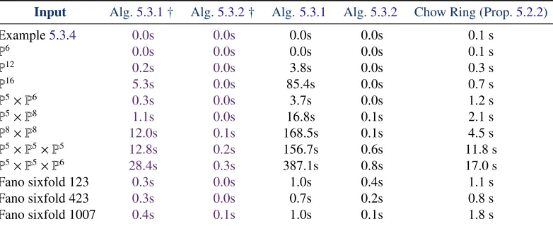
5.4 Performance . . . 141
6 B´ezout Type results in Multi-Projective Space For Application to Au-tomated Polynomial System Solving 145 6.1 Review. . . 147
6.2 B´ezout-like Results . . . 151
6.3 Applications . . . 153
6.3.1 Relations Between the Geometric Multiplicity and Other Multiplicity Functions . . . 154
6.3.2 Affine Varieties with a Bi-projective Structure . . . 158
7 Conclusion 165 A Overview of Implementations and Lists of Examples 170 A.1 Overview of the Implementation used in Chapter 2 and Chapter 3 . . 170
A.2 Examples From Chapter 2. . . 172
A.3 Examples From Chapter 3 . . . 174
A.4 Overview of the Implementation used in Chapter 4 . . . 177
A.5 Examples From Chapter 4. . . 179
A.6 Overview of the Implementation used in Chapter 5 . . . 182
List of Tables
2.1 Comparision of algorithms to compute the Segre class of a sub-scheme ofPn . . . 67
2.2 Comparison of algorithms to compute thecS M class of a subscheme
ofPnusing inclusion/exclusion . . . 70
3.1 Run time results for Algorithm 3.2.2 working overQ . . . 90 3.2 Run time results for Algorithm 3.2.2 working over the finite field
GF(32749). . . 93
4.1 Comparision of algorithms to compute the Segre class of a sub-scheme ofPn1 × · · · ×Pnm . . . 118
4.2 ThecS M class and Euler characteristic in multi-projective space . . . 119
4.3 ThecS M class and Euler characteristic of certain compmplete
inter-sections in multi-projective space . . . 119
5.1 ThecS M class and Euler chacteristic of compete simplicial toric
List of Appendices
Chapter 1
Introduction
The subject matter of this thesis focuses on two separate but related areas of work.
The first area, and that which makes up the bulk of the work, is the computation of
characteristic classes. This is the focus of Chapters2, 3, 4and5. Chapter6gives
the proof of several B´ezout-like bounds in multi-projective space with a focus on their application to obtaining refined running time bounds for solving systems of
polynomial equations in multi-projective space.
The thesis focuses on the use of intersection theory in computer algebra and on
the use of computer algebra to perform computations in intersection theory and algebraic geometry. In Chapters 2, 3, 4 and 5 we use this interplay to construct
algorithms for use on a computer algebra system that will allow us to compute
important invariants in algebraic geometry by solving zero dimensional polynomial
systems in the case of Chapters 2, 3 and 4 and by exploiting the combinatorics
of certain algebraic structures in the case of Chapter 5. In Chapter 6 we use this
interplay to give us refined degree bounds for affine and projective varieties which can be applied to bound the degrees of the polynomial systems arising in problems
in computer algebra.
Macaulay2 [19] implementations of all algorithms for computing characteristics
ters 2and 3 are given as part of the “CharClassCalc” package, package syntax is discussed in Appendix A.1. The Macaulay2 [19] implementations for the
algo-rithms from Chapter4 are given in the “MultiProjChar” package, package syntax
is discussed in AppendixA.4. A Macaulay2 [19] implementation of the algorithms
presented in Chapter5is given in the “CharToric” package, package syntax is
dis-cussed in AppendixA.6.
1.1
Overview of Contributions
We now give a short overview of the contributions presented in this thesis. We
begin by discussing our contributions to algorithms which compute characteristic
classes of algebraic varieties. Next we give an overview of our work on
B´ezout-like bounds in multi-projective space. In this section, we will use some terms not
defined until later; we do this to allow us to give a simple summary of the main
results of the thesis. Complete definitions and more details will be given in the
following sections.
In this chapter and in the following chapters we shall frequently employ the
lan-guage of schemes rather than varieties when working with algebraic geometric
ob-jects. In the statements of the results given the reader may freely mentally substitute
the word “scheme” with the word “variety” and the word “subscheme” with
“sub-variety” and so on, if desired. An overview of the scheme theoretic terminology
used here can be found, for example, in Gathmann [17] or in Eisenbud and Harris [11].
1.1.1
Computing Characteristics Classes
Beginning with Euler’s Polyhedral Formula (circa 1750) the Euler characteristic has
developed into an important invariant for the study of topology and geometry in a
classi-fication of orientable surfaces, the Euler characteristic is an important component in many results in geometry. More recently several authors have noted applications of
the Euler characteristic of projective varieties to problems in statistics and physics.
Specifically the Euler characteristic is used when studying problems of maximum
likelihood estimation in algebraic statistics by Huh in [22] as well as in the study of
problems in string theory by Aluffiand Esole in [6] and by Collinucci, Denef, and Esole in [9].
LetV be a subscheme of a projective spacePn (overkan algebraically closed field of characteristic zero). One of the first computational approaches to calculate the
Euler characteristic of V, χ(V), was to do so by computing Hodge numbers and using the fact that the Euler characteristic is an alternating sum of Hodge numbers.
This approach is implemented in Macaulay2 [19] as the function euler, where the
Hodge numbers are found by computing the ranks of the appropriate cohomology
rings. This approach, however, has significant drawbacks in both applicability and performance. Specifically, this method is only applicable for smooth subschemes
and the computation of the cohomology rings and their respective ranks required to
determine the Hodge numbers is computationally expensive.
Alternatively, one may obtain the Euler characteristic ofV ⊂ Pn
directly from the Chern-Schwartz-MacPherson class of V, cS M(V). In particular, when we consider
cS M(V) as an element of the Chow ring ofPn,A∗(Pn), we have thatχ(V) is equal to the degree of the zero dimensional component of cS M(V). This is the method we shall use to obtain the Euler characteristic. This technique has been used by several
authors (e.g. [2], [23], [21]) to construct different algorithms which are capable of calculating Euler characteristics of complex projective varieties. These previous
methods will be discussed below.
In addition to containing the Euler characteristic, cS M classes are an important in-variant in algebraic geometry, providing a generalization of the Chern class to
sin-gular schemes. While there are several other generalizations of the Chern class to
the relation between Chern classes and the Euler characteristic. Additionally the
cS M class has unique functorial properties (see Definition 2.1.2) and relationships to other common invariants. The cS M class has also found direct applications to problems from string theory in physics, see for example Aluffiand Esole [5].
The existence of a functorial theory of Chern classes for singular varieties, in terms of a natural transformation from the functor of constructible functions to some nice
homology theory, and its relation to the Euler characteristic, was conjectured by
Deligne and Grothendieck in the 1960’s. In the 1974 article [26], MacPherson
proved the existence of such a transformation, introducing a new notion of Chern
classes for singular algebraic varieties. Independently in the 1960’s Schwartz [28]
defined a theory of Chern classes for singular varieties in relative cohomology. It
was later shown in a paper of Brasselet and Schwartz [8] that these two different notions were in fact equivalent.
The problem we consider in Chapters 2and 3 is the following. Letk be an alge-braically closed field of characteristic zero. Given an idealI ink[x0, . . . ,xn] which defines a subschemeV = V(I) in the projective spacePn, how does one compute the Segre class ofVinPn, s(V,Pn), the Chern-Schwartz-MacPherson class ofV,cS M(V) (or Chern classcS M(V)=c(TV)·[V] ifV is smooth) and the Euler characteristic of
V,χ(V)? Further, how does one compute these invariants in a time efficient manner using a computer algebra system?
Our contributions to the resolution of these questions are described in Chapter2and
Chapter3. We give a new expression for the projective degrees of a rational map in Theorem2.3.1. Applying this theorem we give a new algorithm to compute the
projective degrees using a computer algebra system in Algorithm2.3.1. In Chapter
2we use Algorithm2.3.1to give a method to compute the Segre class ofV (Algo-rithm2.3.2) and a method to compute thecS M class and/or Euler characteristic ofV (Algorithm2.3.3). These algorithms are then tested on a wide variety of examples
and are found to perform favourably in comparison to other known algorithms. The
running time results of our algorithms for these examples are summarized in Tables
in§2.4.3.
In Chapter3we give Algorithm3.2.1, a new algorithm to compute thecS M class of a complete intersection subscheme ofPnwith a specific structure. Similar to the
al-gorithms in Chapter2this procedure will also use our method to compute projective
degrees (Algorithm2.3.1). Algorithm 3.2.1offers a significant speed up on some examples. We generalize this method to any complete intersection subscheme ofPn
in Algorithm 3.2.2. The new algorithms are tested on an wide selection of
exam-ples and found to offer considerable performance improvements for many complete intersection varieties, particularly those defined by an ideal I having the property that the majority of the generators of I defined a smooth hypersurface in Pn when considered separately.
The Macaulay2 [19] and Sage [29] implementations of our algorithm for
comput-ingcS M classes, Euler characteristics and Segre classes of subschemes of projective space can be found at https://github.com/Martin-Helmer/char-class-c
alc. The Macaulay2 [19] implementation is also available as part of the
“Char-acteristicClasses” package in Macaulay2 version 1.7 and above and can be
ac-cessed using the option “Algorithm=>ProjectiveDegree”, see the Macaulay2 docu-mentationhttp://www.math.uiuc.edu/Macaulay2/doc/Macaulay2-1.7/sh
are/doc/Macaulay2/CharacteristicClasses/html/for further details.
In Chapter 4we generalize all of the algorithms to compute characteristic classes
for subschemes of projective space described in Chapters 2 and 3 to the
multi-projective setting.
The main results of Chapter 4 are Theorem 4.2.1 and Theorem 4.2.2. Theorem 4.2.1provides a new expression for the Segre classs(V,P) in terms of certain Chow ring elements which may be computed directly from the projective multi-degrees
(which generalize the projective degrees to the multi-projective setting). The result
of Theorem4.2.1generalizes a previous result of Aluffi[2], given below as Proposi-ton2.2.1, which gives an expression for the Segre classes inPn. In Theorem4.2.1
we give a new method to compute the projective multi-degrees which can be easily
implemented on a computer algebra system. These results allow us to construct
algorithms which computes(V,Pn1× · · · ×Pnm),cS M(V) andχ(V) forVa subscheme ofPn1 × · · · ×Pnm.
In Chapter 5 we present Algorithm 5.3.1 which gives a combinatorial algorithm
to compute the Chern-Schwartz-MacPherson class and Euler characteristic and
Al-gorithm 5.3.2 which gives a combinatorial algorithm to compute only the Euler
characteristic of a complete simplicial toric varietyXΣspecified by a fanΣ.
Both Algorithm5.3.1and and Algorithm5.3.2are strictly combinatorial, since they
use only the structure of the fanΣto compute thecS M class and Euler characteris-tic. As such the running times of the algorithms are not dependent on the algebraic
degrees of the defining equations of the variety XΣ. Additionally, unlike the algo-rithms presented in previous chapters, Algorithm5.3.1and Algorithm5.3.2do not
require us to use Gr¨obner bases or other polynomial system solving tools to find
cS M(XΣ).
The main ingredient in the construction of these algorithms is a result of Barthel, Brasselet and Fieseler [7] which we state in Proposition 5.3.1below. This result
gives an expression forcS M(XΣ) in terms of the Chow ring classes of the orbit clo-sures. These Chow ring classes can be easily computed in the case of complete
simplicial toric varieties using standard results such as Theorem 12.5.2. of Cox,
1.1.2
B´ezout-like Results in Multi-projective Space
The problem originally investigated by B´ezout considered the number of
intersec-tion points of two algebraic curves in the plane. In 1916 Macaulay [25] published
a more general result giving the number of intersection points of n hypersurfaces which intersect transversally in Pn as the product of the degrees of the
hypersur-faces. In the modern literature, the term B´ezout theorem is used to refer to a wide class of theorems concerning the intersections of arbitrary varieties or schemes in
a certain projective space,Pn, and in particular to bound, or give an expression for,
the degree of the intersection scheme.
For two intersecting curves in the projective plane, B´ezout’s theorem tells us that the number of points in the intersection counted with multiplicity is equal to the
product of the degrees of the curves. Results of this type in projective space Pn
have been studied intensively both classically and in modern algebraic geometry
and intersection theory. A typical statement of a B´ezout bound for subvarieties
V1, . . . ,Vr ofPn can be found, for example, in Fulton [16, §8.4.6]. LetW1, . . . ,Wt be the irreducible components of∩r
i=1Vi, then we have: t
X
i=1
deg(Wi)≤
r
Y
i=1
deg(Vi). (1.1)
B´ezout type bounds in bi-projective, Pn1 ×Pn2, and multi-projective space, Pn1 ×
· · · ×Pnm have proved to be both more nuanced and more difficult, partially due to
the more complicated structure of the Chow ring. While there are several results
that one could call “a B´ezout type bound” it is not clear that there is one specific
result that one could call “the B´ezout bound” in the multi-projective setting.
The problem we consider in Chapter 6 is the following. Given a collection of
hypersurfaces V1, . . . ,Vr in the multi-projective space Pn1 × · · · ×Pnm defined by multi-homogeneous polynomials, how do we bound the degrees of the sum of the
multi-surfacesV1, . . . ,Vr? We also investigate how such a bound can be constructed in such a way as to give a refined bound on the degree of the irreducible components
(with multiplicity) of a given affine or projective variety with an inherent multi-projective structure. Further, we would like our result to be phrased in such a way
as to be advantageous for use to obtain complexity bounds on algorithms in
com-puter algebra, and hence we would like the terms in the upper bound to be easily
computable and for the notion of multiplicity to be compatible with existing results
giving complexity bounds for solving systems of polynomial equations.
The motivating example for the work in Chapter 6 comes from a problem
con-sidered by Safey El Din and Trebuchet in [13] when developing an algorithm to
compute at least one point in each connected component of a smooth real algebraic
set. The type of systems considered by the algorithm of [13] have a natural
bi-projective structure, because of this using the bi-bi-projective B´ezout-like results of
Chapter6will give a sharper degree bound than using the usual projective B´ezout bound.
1.2
Review and Previous Work
In this section we establish the setting for this work and discuss several previous
results we will employ in later sections as well as discuss some previous algorithms
to compute characteristic classes in projective spaces.
1.2.1
The Setting
A locally ringed space (X,OX) is a pair consisting of a topological space X and a sheaf of rings OX all of whose stalks are local rings. An affine scheme is a lo-cally ringed space which is isomorphic to the spectrum of a commutative ring.
By the spectrum of a commutative ring R we mean the set of all prime ideals in
An Spec(k[x1, . . . ,xn]) as an affine scheme forksome algebraically closed field of characteristic zero. A schemeis a locally ringed space X covered by open sets
Ui such that the restriction of the structure sheaf OX to each Ui is isomorphic to an affine scheme. Put another way a scheme is obtained by glueing together affine schemes in the Zariski topology. The example of a scheme obtained by glueing
affine schemes which we will most frequently use is that of a projective space
Pn = Proj(k[x0, . . . ,xn]) (overkan algebraically closed field of characteristic zero) which we can think of as a scheme obtained by glueing the affine schemesAn. For a more complete discussion see, for example, Gathmann [17] or Eisenbud and Harris
[11].
Characteristics classes will be considered as elements of some Chow ring. The Chow ring of a smooth (irreducible) varietyMwill be denotedA∗(M). For a general definition see§2.1.1. When working with Chow groups and Chow rings byvariety
we will mean a reduced and irreducible scheme. A subvariety of a scheme will be taken to mean a reduced and irreducible subscheme.
In Chapters2and3we considerV = V(I) to be a subscheme of a projective space Pn over an algebraically closed field of characteristic zero defined by a homoge-neous ideal I ink[x0, . . . ,xn]. The characteristics classescS M(V) and s(V,Pn) will be represented as elements of the Chow ring ofPn,
A∗(Pn).
The Chow ring of Pn may be expressed as A∗(Pn) Z[h]/(hn+1) where h is the rational equivalence class of a hyperplane inPn, hence a hypersurfaceW of degree
dinPn is represented as [W]= d·hinA∗(Pn). We will always use the presentation Z[h]/(hn+1) to represent the Chow ringA∗(Pn), and hence s(V,Pn) andcS M(V) will be polynomials in h with the term containing hn representing the dimension zero (codimensionn) component,hn−1representing the dimension one (codimensionn− 1) component and so on.
The Euler characteristic will be given as an integer and is equal to the degree of zero
representation ofcS M(V). We will express this as
χ(V)=
Z
cS M(V).
In Chapter 4 and Chapter 6 we will frequently work in the Chow ring of
multi-projective space P = Pn1 × · · · ×Pnm. The Chow ring of
Pn1 × · · · ×Pnm may be
expressed as
A∗(Pn1 × · · · ×Pnm)Z[h1, . . . ,hm]/(h n1+1
1 , . . . ,h nm+1
m ), (1.2)
wherehi is the rational equivalence class of a general hyperplane inPni (more pre-ciselyhi is the rational equivalence class of the pullback under the projection map Pn1 × · · · ×Pnm →Pni of a general hyperplane inPni) fori=1, . . . ,m.
Let V = V(I) be a subscheme of multi-projective space Pn1 × · · · ×
Pnm over an algebraically closed field of characteristic zero. The characteristics classescS M(V) ands(V,Pn1×· · ·×
Pnm) which we compute in Chapter4will be expressed as elements
of the Chow ringA∗(Pn1×· · ·×Pnm). As with the projective case we may immediately obtain the Euler characteristic fromcS M(V). Specifically we have that
χ(V)=
Z
cS M(V),
which means that χ(V) will be equal to the integer coefficient of hn1
1 · · ·h nm
m in
cS M(V), wherecS M(V) is considered as an element of the Chow ringA∗(Pn1 × · · · × Pnm).
For a complete simplicial toric varietyXΣdefined by a fanΣthe classcS M(XΣ) will be considered as a class in the rational Chow ring A∗(XΣ)Q of XΣ. The structure of this Chow ring is determined by the structure of the fan Σ. For a definition see
1.2.2
The Segre Class
The Segre class is an important invariant in intersection theory in algebraic
ge-ometry, both because it contains important intersection theoretic information and
because it can be used to construct other commonly studied structures and
invari-ants. For example, forV an irreducible subvariety of a variety W the Segre class
s(V,W) contains the Samuel (or algebraic) multiplicity ofV inW (see Fulton [16,
§4.3]). Additionally the Segre class is important in Fulton’s construction of the intersection product ([16, §6]) in the Chow ring and important invariants such as the Chern-Fulton and the Chern-Fulton-Johnson class (in some contexts, see (3.3))
and the Chern-Schwartz-MacPherson class (see Proposition4.1.2) may be defined
in terms of Segre classes.
ForV a proper closed subscheme of a varietyW, we may define the Segre class of
V inW as
s(V,W)=X j≥1
(−1)j−1η∗( ˜Vj)=η∗
[ ˜V] 1+[ ˜V]
!
∈ A∗(V) (1.3)
where ˜V is the exceptional divisor of the blow-up ofW alongV, BlVW,η: ˜V → V is the projection, the class ˜Vkis thek-th self intersection of ˜Vand [ ˜V] is the class of
˜
V in the Chow ring of the blow-up, A∗(BlVW). See Fulton [16, §4.2.2] for further details.
We note that any algorithm to compute the Segre class will immediately give us an
algorithm to compute the Chern-Fulton classcF (refered to as the Canonical class by Fulton [16]) of a subschemeVof a smooth variety Mover an algebraicly closed feild. Specifically we have that
cF(V)=c(TM)·s(V,M)∈A
∗
(M). (1.4)
The Chern-Fulton classcFis a generalization of the Chern class to singular schemes, see, for example, Fulton [16, Examples 4.2.6, 19.1.7]. In particular then, any
[12, Remark 4.2] and Remark3.1.2below.
Previously algorithms have been given by Allufi [2] and by Eklund, Jost, and
Pe-terson [12] to compute the Segre class inPn. To compute s(V,Pn) the algorithm of Allufi [2] requires the computation of the blowup of Pn along V, i.e. requires the computation of the Rees algebra. This is an expensive operation in general. The al-gorithm of Eklund, Jost, and Peterson [12] works by computing certain residual sets
via saturation and then computing their degrees. For a more detailed comparison of
these methods with our method using projective degrees see Chapter2.
In the multi-projective setting a previous algorithm of Moe and Qviller [27] which computes the Segre class of a subscheme of a smooth projective toric variety could
be applied. This algorithm generalizes the algorithm of Eklund, Jost, and Peterson
[12]. The algorithm of Moe and Qviller [27], however, does not make use of the
special structure of the Chow ring of multi-projective space and hence performs
extra, unnecessary, computations in the multi-projective case. A performance
com-parison with our algorithm to compute the Segre class inPn1× · · · ×Pnm can be found in Table4.1.
1.2.3
The Chern-Schwartz-MacPherson Class and the Euler
Char-acteristic
A general definition of the Chern-Schwartz-MacPherson class is given in Definition
2.1.2. Rather than giving the general definition here we instead focus on giving a more intuitive understanding of the geometric information contained in the cS M class and on some methods for its computation. Note that in this subsection, for
simplicity, we will restrict our discussion to subschemes ofPn.
cS M(V) we may directly obtain the list of invariants
χ(V), χ(V∩L1), χ(V∩L1∩L2), . . . , χ(V∩L1∩ · · · ∩Lm)
where L1, . . . ,Lm are general hyperplanes. Conversely from the list of Euler char-acteristics above we could obtaincS M(V), i.e. there exists an involution between the Euler characteristics of general linear sections and thecS Mclass in this setting. This relationship is given explicitly in Theorem 1.1 of Aluffi[4]; we give an example of this below.
Example 1.2.1.Consider the subvariety ofP4given by V= V(4x
3x2x4x1−x30x1,x0x1x3x4− x3
2x3). In Example 1.3.2we will compute that cS M(V) = 5h
4 +8h3 +12h2. To ob-tain the Euler characteristics of the general linear sections of V we may apply an involution formula given by Aluffiin [4, Theorem 1.1], specifically:
• First consider the polynomial p(t) = 5+8t+ 12t2 ∈
Z[t]/(t5) given by the
coefficients of the cS M class above.
• Next apply Aluffi’s involution
p(t)7→ I(p) := t· p(−t−1)+ p(0)
t+1 = 12t
2+4t+5.
This givesχ(V)=5, χ(V∩L1)=(−1)1·4=−4,andχ(V∩L1∩L2)=(−1)2·12=12 where L1and L2are general hyperplanes inP4.
The general result of Aluffi[4] relating thecS M class and the Euler characteristic in Pncan be found below in Theorem2.1.5.
We now discuss the computation ofcS M classes and hence of Euler characteristics of subschemes of projective space, beginning with the case of a hypersurface.
as
cS M(V(f))=(1+h)n+1−
n
X
j=0
gj(−h)j(1+h)n−j inA∗(Pn)Z[h]/(hn+1). (1.5)
This result has been used to yield several different computational methods to cal-culate the cS M class. The differences between the methods lay in how the gj’s are understood and computed. The first algorithm to compute cS M(V(f)) was that of Aluffi [2]. To compute the gj’s this algorithm requires the computation of the blowup ofPn along the singularity subscheme of
V(f) (that is the scheme defined by the partial derivatives of f). Hence the cost of computing thecS M class of a hy-persurface using the method of Aluffiis that of computing the Ress algebra of the ideal defining the singularity subscheme of the hypersurface. This can be a quite
expensive operation, making this algorithm impractical for many examples.
Another algorithm to compute thecS M class of a hypersurface was given by Jost in [23]. This method makes use of Fulton’s residual intersection theorem (Theorem
9.2 of Fulton [16]) which allows Jost to consider thegj’s in (1.5) as the degrees of Fulton’s residual scheme. Jost also shows that in the context of cS M (and Segre) class computations these residual schemes can be computed by finding a particular
saturation. Hence the computation of the saturation to find the residual scheme and
the computation of its degree are the main costs of Jost’s algorithm. The algorithm
of Jost is probabilistic and yields the correct result for a choice of objects lying in an open dense Zariski set of the corresponding parameter space, see Jost [23] or
Eklund, Jost, and Peterson [12].
In Chapter 2 we present Algorithm 2.3.3, in which we consider the gj’s as the projective degrees of a rational map defined by the partial derivatives of f. As with the method of Jost [23] our method is probabilistic and yields the correct result for a
choice of objects lying in an open dense Zariski set of the corresponding parameter
space.
one. Specifically forV1,V2 subschemes of Pn the inclusion/exclusion property for
cS M classes states
cS M(V1∩V2)= cS M(V1)+cS M(V2)−cS M(V1∪V2). (1.6)
This property may easily be extended to computecS M classes of any codimension, see Proposition2.1.3.
While the use of this property allows for the computation ofcS M(V) for V of any codimension, it requires exponentially manycS M computations relative to the num-ber of generators of I. Additionally some of the schemes considered while per-forming inclusion/exclusion may have significantly higher degree than the original schemeV.
1.3
Results
In this section we provide a more detailed introduction to the results presented in
this thesis. For the introduction we will focus on presenting examples where
possi-ble.
1.3.1
Characteristic Class Computations in
P
nThe main result of Chapter 2 is Theorem 2.3.1which gives an expression for the
projective degrees of a rational map associated to a homogeneous ideal. We use
this result to construct Algorithm2.3.1which computes the projective degrees of a
rational map defined by an ideal. We then use Algorithm2.3.1to construct
Projective Degrees of a Rational Map
Consider a rational map φ : Pn d Pm. In the manner of Harris (Example 19.4
of [20]) we may define the projective degrees of the map φ as a list of integers (g0, . . . ,gn) where
gi =card
φ−1
Pm−i
∩Pi, (1.7)
where Pm−i ⊂ Pm and Pi ⊂ Pn are general hyperplanes of dimension m− i and i respectively and card is the cardinality of a zero dimensional set.
We give a method to compute the projective degrees of a rational map in Theorem
2.3.1below. This method will form the basis for our algorithms to compute
charac-teristic classes for subschemes ofPn. LetI = (f0, . . . , fm) be a homogeneous ideal ink[x0, . . . ,xm]; if we consider a rational mapφ:Pnd Pmassociated to the idealI which is defined by,
φ: p7→(f0(p) :· · · : fm(p)),
then Theorem2.3.1tells us thatg0 =1 and that
gi = dimk(k[x0, . . . ,xn,T]/(P1+· · ·+Pi+L1+· · ·+Ln−i+LA+S)). (1.8)
Here P`,L`,LA and S are ideals ink[x0, . . . ,xn,T]; the ideals P` are generated by a general linear combination of f0, . . . , fm, the ideals L` are generated by general homogeneous linear forms in k[x0, . . . ,xn], the ideal LA is generated by an affine linear form ink[x0, . . . ,xn] and the idealS is given by
S =
1−T
m X
j=0 λjfj
,
wherePm
j=0λjfj is a general linear combination of f0, . . . , fm.
We use this result to construct a probabilistic algorithm to compute the projective
degrees of a rational map specified by an ideal in Algorithm2.3.1. The algorithm will give the correct result for a general choice of constants, i.e. for constants ink
Segre Classes
Assume that V is a subscheme of Pn over k, an algebraically closed field of char-acteristic zero, and that V is defined by a homogeneous ideal I = (f0, . . . , fm) in k[x0, . . . ,xn]. Adapting Proposition 3.1 of Aluffi[2] (given as Proposition2.2.1 be-low) to this case we have that the Segre classs(V,Pn) can be written in terms of the projective degrees of the rational map associated to the idealI.
In Algorithm2.3.2 we give a method to compute the Segre class s(V,Pn) for V a subscheme of Pn from the projective degrees of the rational map associated to I. Specifically our algorithm first computes the projective degrees by applying
Algo-rithm2.3.1and then uses these to constructs(V,Pn) using Proposition2.2.1.
We give an example illustrating the process used by Algorithm 2.3.2in Example
1.3.1below.
Example 1.3.1. Let V = V(I) be the subvariety of P4 defined by the ideal I = (4x3x2x4x1−x03x1,x0x1x3x4−x32x3)=(f0, f1)in k[x0,x1,x2,x3,x4]. V has dimension two and the singularity subscheme of V also has dimension two (by singularity subscheme we mean the subscheme of V defined by the2×2minors of the Jacobian matrix of I). Also set d= deg(f0)=deg(f1)=4.
Recall that we may write the Chow ring ofPnas A∗(Pn)Z[h]/(hn+1)where h is the
rational equivalence class of a hyperplane, meaning a hypersurface W of degree d inPn is represented as[W]= d·h in A∗(
Pn).
We first compute the Segre class s(V,P4) of V in P4 considered as an element of
A∗(P4) Z[h]/(h5). We will follow the procedure of Algorithm2.3.2. This algorithm
is probabilistic in the same manner as Algorithm2.3.1, our algorithm for computing projective degrees. Consider the rational mapφ : P4
d P1 defined by the ideal I,
that is
φ: p7→(f0(p) : f1(p)).
that g0 =1and that we may compute
g1 = dimk(R/(P1+L1+L2+L3+LA+S))
where P1 = (7f0+9f1)is the ideal in R defined by a general linear combination of the generators of I;
L1 = (−11x0+21x1−3x2−18x3+22x4) L2 = (31x0−23x1+2x2+47x3−43x4) L3 = (13x0−52x1−29x2+71x3−15x4)
are ideals in R defined by general homogeneous linear forms in k[x0,x1,x2,x3,x4],
LA =(17−14x0+41x1+12x2−91x3−3x4)
is an ideal in R defined by an affine general linear form in k[x0,x1,x2,x3,x4], and S is the ideal of R given by S = (1−T(3f0− 5f1)). The expression 3f0 −5f1 in the definition of S is a general linear combination of the generators of I. This gives g1 = 4. In a similar manner we may compute the remaining projective degrees to obtain
(g0,g1,g2,g3,g4)=(1,4,0,0,0).
Applying the formula in(2.24)expressing the Segre class in terms of the projective degrees we obtain
s(V,Pn)=1− n
X
i=0
gihi (1+dh)i+1 =1− 1
1+4h −
4h
(1+4h)2
=768h4−128h3+16h2∈A∗(P4).
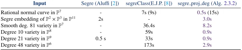
the projective degrees (Algorithm 2.3.2) to other known algorithms and find that in most cases Algorithm 2.3.2performs favourably. In Corollary 2.4.2we give a
running time bound for Algorithm2.3.2. The other known algorithms to compute
Segre classes do not have known running time bounds.
The Chern-Schwartz-MacPherson Class and the Euler Characteristic
In Algorithm2.3.3we present an algorithm to computecS M classes using the pro-jective degrees and inclusion/exclusion. Running time bounds for this algorithm are given in Corollary2.4.3. The other known algorithms to computecS M classes do not have known running time bounds.
We now give an example of computing thecS M class and Euler characteristic using Algorithm2.3.3.
Example 1.3.2. As in Example1.3.1we take V = V(I)be the subvariety ofP4
de-fined by the ideal I =(4x3x2x4x1−x03x1,x0x1x3x4−x23x3)= (f0, f1)in k[x0,x1,x2,x3,x4]. By the inclusion/exclusion property of cS M classes(1.6)we have that
cS M(V)=cS M(V(f0))+cS M(V(f1))−cS M(V(f0· f1)). (1.9)
We first calculate cS M(V(f0)); we begin by finding the projective degrees of the map corresponding to the ideal J generated by the partial derivatives of f0
J= (∇f0)=(3x20x1,−x30+4x2x3x4,4x1x3x4,4x1x2x4,4x1x2x3),
that is we must find the projective degrees (g0,g1,g2,g3,g4) of the rational map ϕ:P4 dP4(sometimes referred to as the polar or gradient map(2.18)) given by
ϕ: (p0 : p1 : p2 : p3 : p4)7→(3p20p1:−p30+4p2p3p4 : 4p1p3p4 : 4p1p2p4: 4p1p2p3).
we computed g1= 3. Now compute
g2 = dimk(k[x0,x1,x2,x3,x4,T]/(P1+P2+L1+L2+LA+S)),
where P1 and P2 are the ideals in R generated by a general linear combination of the generators of J; L1,L2 are ideals of R generated by homogeneous linear forms in k[x0,x1,x2,x3,x4]and LAis an ideal in R given by a general affine form in
k[x0,x1,x2,x3,x4]and finally S is the ideal in R given by
S =1−T7(3x02x1)+15(−x30+4x2x3x4)−13(4x1x3x4)+24(4x1x2x4)−3(4x1x2x3)
.
This gives g2 = 6. Again applying Corollary 2.3.3 we find the other projective degrees are(g0,g1,g2,g3,g4)=(1,3,6,6,2). By(1.5)this gives us that
cS M(V(f0))=(1+h)n+1− n
X
j=0
gj(−h)j(1+h)n−j
=(1+h)5−
4
X
j=0
gj(−h)j(1+h)4−j =5h4+9h3+7h2+4h∈A∗(P4).
Similarly we find that the projective degrees corresponding to f1, and f0f1 are (1,3,6,6,2)and(1,7,23,29,12)respectively. This gives the cS M classes:
cS M(V(f1))=5h4+9h3+7h2+4h, cS M(V(f0f1))=5h4+10h3+2h2+8h.
Combining these we obtain
cS M(V)=5h4+8h3+12h2 ∈A∗(P4)Z[h]/(h5).
From this we may immediatly obtain that the Euler characteristic of V isχ(V)= 5
cS M(V), i.e. the coefficent of h4 in cS M(V)since V ⊂P4.
In Chapter 3 we develop an algorithm to compute the cS M class in codimension higher than one which does not require the use of inclusion/exclusion for certain types of subschemes ofPn. More specifically we give an algorithm that will allow
for the direct computation of the cS M classes of arbitrary, possibly singular, glob-ally complete intersection subschemes ofPndefined by a homogeneous polynomial
idealI =(f0, . . . , fm) where the scheme defined by (f0, . . . , fm−1) is smooth (allow-ing for a possible rearrangement of the generators ofI). This algorithm is described in Algorithm 3.2.1. The main result needed for this algorithm is Theorem 3.2.1
which gives a concrete expression forcS M(V(I)) in terms of the Segre classs(Y,Pn) whereYis the singularity subscheme ofV (that is the subscheme ofVgenerated by (m+1)×(m+1) minors of the Jacobian matrix ofI). The main ingredient in the proof of Theorem3.2.1is a result of Fullwood [14] which gives an expression for
the Milnor class in this case; this result is given as Theorem3.1.1below.
We now given an example of using this result in the manner presented in Algorithm
3.2.1to compute thecS M class.
Example 1.3.3. Let I =(3x30+5x31+2x32−9x33+7x43,−x22x23+x0x1x24)= (f0, f1)and let V = V(I), compute cS M(V)using Algorithm3.2.1. Note that V(3x30+5x31+2x32− 9x33+7x34)is smooth, hence Algorithm3.2.1can be used directly. First compute the singularity subscheme Y of V, the Jacobian matrix of I is:
Jac(I)=
9x20 15x21 6x22 −27x23 21x24 x1x42 x0x24 −2x2x23 −2x22x3 2x0x1x4
letJ be the ideal generated by the˜ 2×2minors ofJac(I)and compute
J =( ˜J+I) : (x0,x1,x2,x3,x4)∞ =(x1x24,x0x24,x2x3x4,x0x1x4,x2x32,x
2
2x3,3x30+5x 3 1+2x
3 2−9x
3 3+7x
3 4)
Hence we have that Y =V(J)is the singularity subscheme of V. Note thatdimY =
P4 d P6 defined by the ideal J, we may compute these projective degrees using
Theorem2.3.1, for this example we will show the computation of g3.
Let R= k[x0,x1,x2,x3,x4,T]; from Theorem2.3.1we have
g3 =dimk(R/(P1+P2+P3+L1+LA+S)), (1.10)
where P1,P2,P3 are ideals in R defined by general linear combinations of the gen-erators of J, L1 is an ideal in R defined by a general homogeneous linear form in k[x0,x1,x2,x3,x4], LA is an ideal in R defined by a general affine linear form in
k[x0,x1,x2,x3,x4]and S is the ideal in R defined by S =(1−T(λ0J0+· · ·+λ6J6)) where J0, . . . ,J6 are the generators of J and λ0J0+ · · ·+λ6J6 is a general linear combination. This gives g3 =21; the remaining projective degrees may be obtained in a similar fashion, giving (g0,g1,g2,g3,g4) = (1,3,9,21,24). Now using (2.24) as in Algorithm3.2.1we obtain
s(Y,P4)=1− 4
X
i=0
gihi (1+3h)i+1 =−15h4+6h3 ∈A∗(P4).
In the notation of Theorem 3.2.1 this gives (s0,s1,s2,s3,s4) = (0,0,0,6,−15). Again using the notation of Theorem 3.2.1 we note that Q1
i=0(1 + deg(fi)h) = (1+3h)(1+4h) = 12h2+7h+1, hence we have thatc˜
0 = 1,c˜1 = 7andc˜2 = 12. We may now calculate cS M(V)by applying Theorem3.2.1, this gives
cS M(V)= (1+h)5· 3h
1+3h ·
4h
1+4h+
(1+h)5 (1+3h)(1+4h)
2 X
p=0 hp
p
X
i=0
2+1−i p−i
!
(−1)i4p−i·c˜i
· 4 X
i=0
(−1)is ihi (1+4h)i
.
Simplifying we obtain
The Euler chacteristic χ(V) = 81 is given by the degree of the zero dimensional component of cS M(V).
In Proposition3.2.2we give a modified version of the inclusion/exclusion property which considers only the singular generators of an ideal, specifically we show the
following. LetZ ⊂ Pn
be smooth (scheme-theoretically) and let X1 = V(f1), X2 = V(f2) be singular hypersurfaces inPn. IfV =Z∩X1∩X2, then we have
cS M(V)=cS M(Z∩X1)+cS M(Z∩X2)−cS M(Z∩(X1∪X2)), (1.11)
hereX1∪X2is the scheme generated by f1· f2. Additionally, whenV is a complete intersection each of the terms in (3.9) can be computed using Theorem3.2.1.
Using this result and Algorithm 3.2.1 we devise Algorithm 3.2.2 which is
appli-cable for any globally complete intersection subscheme of Pn. Algorithm 3.2.2
uses the specialized version of inclusion/exclusion (1.11) to break up thecS M class computation into a sum ofcS M classes of objects which satisfy the assumptions of Theorem3.2.1, i.e. where there exists a smooth scheme defined by all but one of the generators. Each of these cS M classes can then be computed with Algorithm 3.2.1.
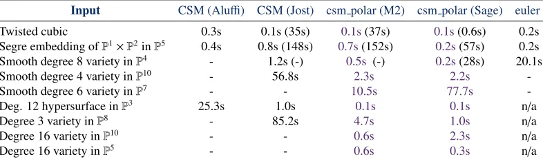
In Table3.1 and Table3.2we test Algorithms 3.2.1and3.2.2 on a wide selection
of complete intersection subschemes ofPn. We find that Algorithms3.2.1and3.2.2 perform favourably in comparison to other algorithms which computecS M(V) class on many applicable examples, with the largest speed up happening when the
ma-jority of the generators of the ideal defining the schemeV are smooth. We also note that the speed up over our inclusion/exclusion based algorithm is quite significant in some cases. If, however, many of the generators define a singular scheme then
Algorithms3.2.1does not necessarily offer improved performance in comparison to inclusion/exclusion as the cost of computing the singularity subschemes and their Segre classes can become too large. All things considered we believe that
1.3.2
Characteristics Class Computations in
P
n1× · · · ×
P
nmThe main results in Chapter4are Theorem4.2.1and Theorem4.2.2. Theorem4.2.2
gives a method to compute the so-called projective multi-degrees, i.e. the analogue
of the projective degrees of (1.7) in multi-projective space (see (4.9)). Theorem
4.2.1generalizes a result of Aluffi[2] and gives an expression for the Segre class in
Pn1 × · · · ×Pnm in terms of Chow ring classes which can be computed directly from the projective multi-degrees of (4.9), these can in turn be found using Theorem
4.2.2.
Projective Multi-degrees
Theorem 4.2.2generalizes the result of Theorem 2.3.1; we summerize this result
here. Recall that the Chow ring ofPn1 × · · · ×
Pnm may be expressed as
A∗(Pn1 × · · · ×
Pnm)Z[h1, . . . ,hm]/(h n1+1
1 , . . . ,h nm+1
m ).
Let R be the coordinate ring of Pn1 × · · · × Pnm, let I = (f0, . . . , fr) be a multi-homogeneous ideal inRdefining a subschemeV = V(I) ofPn1 × · · · ×
Pnm and let
n = n1+· · ·+nm. Assume, without loss of generality, that all generators ofI have the same multidegree, that is assume that deg(fi) = (d1, . . . ,dm) for all i. Define a rational mapφ:P→ Prgiven by
φ: p7→(f0(p) :· · ·: fr(p)). (1.12)
Let
G =
codim(V)−1
X
ι=0
(d1h1+· · ·+dmhm)ι+ n
X
ι=codim(V)
[Yι]∈A∗(P), (1.13)
where
[Yι]=
h
V(P1+· · ·+Pι)−V(I)
i
with thePi being general linear combinations of (f0, . . . , fr). Note that [Yι] has pure codimensionι, hence the class [Yι]∈A∗(P) will have the form
[Yι]= X i1+···+im=ι
0≤i1≤n1,...,0≤im≤nm
γ(i1,...,im)h
i1
1 · · ·h im
m. (1.15)
We will refer to the γ(i1,...,im) as the projective multi-degrees of the rational map
φ.
In Theorem4.2.2we show that we may compute the projective multi-degreesγ(i1,...,im)
by computing the the vector space dimensions
γ(i1,...,im)= dimk R[T]/(P1+· · ·+Pι+L(a1,...,am)+LA+S) ,
(1.16)
forι= codim(V), ..,nwhere:
• P1, . . . ,Pιare ideals defined by general linear combinations of the generators ofI, i.e.
Pj =
r X
l=0 λj,lfl
.
• S is an ideal given by
S = 1 −T r X
l=0 ϑlfl
,
wherePr
l=0ϑlflis a general linear combination of f0, . . . , fr.
• L(a1,...,am) is an ideal generated by a1 general homogeneous linear forms of
multi-degree (1,0,0, . . . ,0), a2 general homogeneous linear forms of multi-degree (0,1,0, . . . ,0), and so on.
• LAis the ideal generated by themaffine linear forms
Segre Classes
Let V = V(f0, . . . , fr) be a subscheme of P = Pn1 × · · · ×Pnm. In Theorem 4.2.1 we prove a result which gives an expression for the Segre classs(V,Pn1 × · · · ×Pnm) in terms of the projective multi-degrees (1.15). Using this result and the result
of Theorem 4.2.2 we construct Algorithm 4.3.1 which computes the Segre class
s(V,P) by constructing the classes [Yι] as in (1.15). The main computational steps of Algorithm 4.3.1are the calculations of the vector space dimensions to find the
projective multi-degreesγ(i1,...,im)in (1.16).
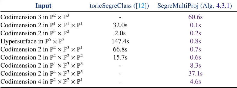
In Table4.1 we compare the run time of our new algorithm to compute the Segre
class of a subscheme of multi-projective space to the algorithm of Moe and Qviller [27], which is also capable of computing Segre classes in this setting, for a variety of
examples. We find that in all cases our method of Algorithm4.3.1offers superior run time performance and that for the majority of the examples the difference in performance is considerable. We note that the algorithm of Moe and Qviller [27]
works in a more general setting (subschemes of a smooth projective toric variety)
and does not attempt to take advantage of the special structures of the Chow rings
associated to any particular case.
We give a running time bound for our algorithm to compute Segre classes of
sub-schemes of multi-projective space (Algorithm4.3.1) in Proposition4.4.1.
Chern-Schwartz-MacPherson Classes
We give two algorithms to compute the class cS M(V) forV a subscheme of multi-projective space, Algorithm4.3.2and Algorithm4.3.3. Algorithm4.3.2generalizes
using Algorithm4.3.1to compute the Segre class of the singularity subscheme and using the inclusion/exclusion property ofcS M classes in higher codimension.
We give running time bounds for Algorithm 4.3.2 in Corollary 4.4.2. In Table
4.2 we give the running time of our algorithm on several examples. At present
there are no other existing algorithms known to us for computing Chern-Schwartz-MacPherson classes in the multi-projective setting, hence we are unable to compare
these running times to those of another existing algorithm.
In Algorithm 4.3.3 we generalize Algorithm 3.2.1 to the multi-projective setting.
We proceed similarly to the construction for projective space given in Chapter 3, namely we prove Theorem 4.2.3which gives an expression for thecS M class of a complete intersectionV = V(f0, . . . , fr) ⊂Pn1 × · · · ×Pnm whereV(f0, . . . , fr−1) is a smooth scheme (for some ordering) in terms of the Segre classs(Y,Pn1 × · · · ×
Pnm)
of the singularity subscheme Y ofV. As in the projective case to prove Theorem 4.2.3we apply a result of Fullwood [14] which gives an expression for the Milnor
class in this setting. Theorem4.2.3 generalizes the result of Theorem3.2.1to the
multi-projective setting.
Hence Algorithm4.3.3computes thecS M class of a complete intersection satisfying the assumptions of Theorem 4.2.3 without the need for inclusion/exclusion. This algorithm can also be extended to any complete intersection by doing a partial
in-clusion/exclusion in a manner similar to that of Algorithm 3.2.2. Specifically for
Z a smooth subscheme of Pn1 × · · · ×Pnm and for V1,V2 arbitrary subschemes of Pn1 × · · · ×Pnm we have
cS M(Z∩V1∩V2)= cS M(Z∩V1)+cS M(Z∩V2)−cS M(Z∩(V1∪V2))
note that all expressions on the left hand side of the equation above satisfy the
assumptions of Theorem4.2.3.
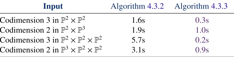
In Table 4.3 we compare the run times of Algorithm4.3.3 to those of Algorithm
of Algorithm4.3.3does indeed offer a performance improvement over inclusion/ ex-clusion. While the set of applicable examples is slightly restricted we believe
that Algorithm 4.3.3 still provides a useful complement to the more general
in-clusion/exclusion method of Algorithm4.3.2.
Note that both these methods to computecS M(V) forVa subscheme ofPn1×· · ·×Pnm also allow us to immediately obtain the Euler characteristic χ(V) from the class
cS M(V) since
χ(V)=
Z
cS M(V).
1.3.3
Computing the Chern-Schwartz-MacPherson Class and
Eu-ler Characteristic of Complete Simplicial Toric Varieties
For a complete simplicial toric varietyXΣdefined by a fanΣ, the classcS M(XΣ) will be considered as a class in the rational Chow ring A∗(X
Σ)Q ofXΣ. A definition of
this Chow ring (which is well suited to computation) is given in§5.2.
We now give an example using Algorithm 5.3.1 and Algorithm 5.3.2to compute
cS M(P3) = c(TP3) · [P
3] in the Chow ring of
P3 and to compute χ(P3). We note that this Chern class and Euler characteristic are, of course, well known and these
algorithms are not required for this computation. Rather this example is chosen to
illustrate the algorithms in a simple way. An example with a singular toric variety is
given as Example5.3.4in Chapter5. For definitions of terms used in this example
see§5.1.
defined by the cones
σ0 =ρ0+ρ1+ρ2 σ1 =ρ0+ρ1+ρ3 σ2 =ρ0+ρ2+ρ3 σ3 =ρ1+ρ2+ρ3
and their faces where ρ0 = h(1,0,0)i, ρ1 = h(0,1,0)i, ρ2 = h(0,0,1)i, ρ3 =
h(−1,−1,−1)i. We may refer toρ0, ρ1, ρ2, ρ3 as the generating raysΣ(1)ofΣ.
The Chow ring ofP3as a toric variety has presentation
A∗(P3) Z[x0,x1,x2,x3]/(x0x1x2x3,x1−x0,x2−x0,x3−x0),
note that the above toric presentation is isomorphic to the usual presentation A∗(P3) Z[h]/(h4), however for this example we will use the toric presentation as in
Algo-rithm 5.3.1. Note that since P3 is smooth we will have mult(σ) = 1 for all cones σ∈Σ, see Lemma5.3.2.
Using Algorithm5.3.1we have that the codimension one part of cS M(P3)is
(cS M(P3))(1) =mult(ρ0)[V(ρ0)]+mult(ρ1)[V(ρ1)]+mult(ρ2)[V(ρ2)]+mult(ρ3)[V(ρ3)]∈A∗(P3) = x0+x1+x2+x3
The codimension two part of cS M(P3)is
(cS M(P3))(2) =mult(ρ0+ρ1)[V(ρ0+ρ1)]+mult(ρ0+ρ2)[V(ρ0+ρ2)] +mult(ρ0+ρ3)[V(ρ0+ρ3)]+mult(ρ1+ρ2)[V(ρ1+ρ2)]
+mult(ρ1+ρ3)[V(ρ1+ρ3)]+mult(ρ2+ρ3)[V(ρ2+ρ3)]∈A∗(P3) = x0x1+ x0x2+x0x3+x1x2+x1x3+x2x3
=6x23.
The codimension three part of cS M(P3)is
(cS M(P3))(3) =mult(ρ0+ρ1+ρ2)[V(ρ0+ρ1+ρ2)] +mult(ρ0+ρ1+ρ3)[V(ρ0+ρ1+ρ3)] +mult(ρ0+ρ2+ρ3)[V(ρ0+ρ2+ρ3)]
+mult(ρ1+ρ2+ρ3)[V(ρ1+ρ2+ρ3)]∈A∗(P3) = x0x1x2+x0x1x3+x0x2x3+ x1x2x3
=4x33.
Finally we note the the codimension zero part of cS M(P3) is 1 ∈ A∗(P3), i.e. the
class of the orbit closure of the zero coneh(0,0,0)iis [V(h(0,0,0)i)] = 1. Hence Algorithm5.3.1gives us
cS M(P3)= 4x33+6x 2
3+4x3+1∈A∗(P3) Z[x0,x1,x2,x3]
(x0x1x2x3,x1−x0,x2−x0,x3−x0) ,
the last step of the algorithm is to find a basis for the dimension zero Chow group A0(P3) and compute the Euler characteristic. In this case
n
x33o forms a basis of A0(P3), hence the Euler characteristic is the coefficient of x33in cS M(P
3), that is
χ(P3)=
Z
cS M(P3)=4.
would perform only the computation of the codimension three piece of the cS M class,
that is the computation of (cS M(P3))(3) above. From this, Algorithm5.3.2 obtains the Euler characteristic directly by summing the coefficients of the monomials in the polynomial expression of(cS M(P3))(3) above, this givesχ(P3)= 4.
1.3.4
B´ezout Type Results in Multi-projective Space
In this subsection we will focus only on motivating the B´ezout-like bounds of
Chap-ter6by considering an example application of the results proved in Chapter6to a
problem considered by Safey El Din and Trebuchet in [13].
In the following we will frequently make use of the notion ofgeometric multiplicity
in the manner of Fulton [16, §1.5] and Fulton [15, §2.1]; we briefly describe this notion here. Let k be an algebraically closed field of characteristic zero. Let V
be a subvariety (or subscheme) of kn = Spec(k[x1, . . . ,xn]), i.e. a subvariety of dimensionnaffine space with coordinate ringk[x1, . . . ,xn]. LetWbe an irreducible component ofV. In this case the local ringOW,V is given by the localization of the coordinate ring ofV at the prime idealI(W), that is
OW,V = (k[x1, . . . ,xn]/I(V))I(W),
see [15,§2.1] or the proof of Lemma 6.3.3, and see §6.1for the definition ofOW,V in a more general setting.
We will write` OW,V
= `
OW,V OW,V
for thegeometric multiplicityofWinVwhere ` OW,Vis the length ofOW,V as anOW,V-module. Recall that a moduleMhas length
nif there is a composition series M0 = M % M1 % · · · % Mn = {0} and this is the shortest such series. For a set of points in affine space the notion of geometric multiplicity defined above reduces to the usual notion of the multiplicity of a point
as we will see in the Example1.3.5.
V = V(f1, . . . , fn)in kn and W = (a1, . . . ,an)an isolated point in V we have
` OW,V=dimk (k[x1, . . . ,xn]/(f1, . . . , fn))P
,
(1.17)
where P=(x1−a1, . . . ,xn−an)is the prime ideal of the point W.
Consider the intersection of two curves f,g inC2 = Spec(C[x,y]), if p = (a,b)is
an isolated point in the intersection V = V(f,g)then
`
Op,V
=dimC(C[x,y]/(f,g))(x−a,y−b)
.
If we take V to be the intersection of the curves y= x2and the x-axis y= 0we have one isolated point at p=(0,0)with geometric multiplicity
`
Op,V
= dimC
C[x,y]/(x2−y,y)
(x,y)
= dimCC[x,y](x,y)/(x2−y,y)
= dimCC[[x,y]]/(x2−y,y)
= 2.
Here the basis ofC[[x,y]]/(x2−y,y)given by{1,x}whereC[[x,y]]denotes the ring
of formal power series. Note that we may replace the localizationC[x,y](x,y)by its completionC[[x,y]]in this case, see Fulton [15,§1.6].
The motivating example for the work in Chapter6 we consider here comes from
a problem considered by Safey El Din and Trebuchet in [13] when developing an algorithm to compute at least one point in each connected component of a smooth
real algebraic set.
collection of polynomials ink[x1, . . . ,xn,l1, . . . ,lm]
Fj =
fj if j≤m
l1 ∂f1
∂xj−m +· · ·+lm
∂fm
∂xj−m −1 if j=m+1
l1 ∂ f1
∂xj−m +· · ·+lm
∂fm
∂xj−m ifm+2≤ j≤m+n
. (1.18)
We may then calculate the critical locus by using an algorithm such as Giusti, Lecerf
and Salvy [18] (or Lecerf [24]) to compute the variety V = V(F1, . . . ,Fn+m). Let
W1, . . . ,Wt be the irreducible components ofV. The algorithms of Giusti, Lecerf and Salvy [18] and of Lecerf [24] have known running time bounds that depend on
the sum of the degrees of theWi weighted by multiplicity, that is the running time bounds depend on the quantityδgiven by
δ= X
`(OWi,V) deg(Wi).
Hence to give refined running time bounds on the time to compute the critical lo-cus ofV(f1, . . . , fm) using the method of Lagrange multipliers the problem we wish to consider is the following. Letting V ⊂ An+m be the affine variety defined by
V = V(F1, . . . ,Fn+m), how do we provide a refined bound on the degrees of the irre-ducible componentsW1, . . . ,WjofVwith multiplicity, i.e. a bound which is sharper than the usual B´ezout bound in this case? More specifically, if we homogenize to
obtain the projective closureV ⊂Pn+mwe could then apply the usual B´ezout bound inPn+mto obtain
δ= j
X
i=1
`(OWi,V) deg(Wi)≤D
n+m.
(1.19)
Our goal is to obtain a sharper bound than this by making use of the natural
bi-projective structure of the variety associated to the system of polynomials in (1.18).
In fact from Corollary6.3.8we have the following bound
δ= j
X
=
`(OWi,V) deg(Wi)≤
n+m−1
n−1
!
Corollary 6.3.8 follows from Theorem 6.2.1 which we prove in Chapter 6. Ad-ditionally ifV(F1, . . . ,Fm) is a complete intersection, Corollary6.3.9gives us the slightly sharper bound
δ= j
X
i=1
`(OWi,V) deg(Wi)≤
n n−m
!
Dm(D−1)n−m.
We note that the bounds obtained from Corollary 6.3.8 and Corollary 6.3.9 are
sharper (at least for large degree) than the bound obtained from the standard
Bibliography
[1] Paolo Aluffi. Chern classes for singular hypersurfaces. Transactions of the American Mathematical Society, 351(10):3989–4026, 1999.
[2] Paolo Aluffi. Computing characteristic classes of projective schemes. Journal of Symbolic Computation, 35(1):3–19, 2003.
[3] Paolo Aluffi. Characteristic classes of singular varieties. InTop. in Cohomo. Studies of Alg. Var., pages 1–32. Springer, 2005.
[4] Paolo Aluffi. Euler characteristics of general linear sections and polynomial Chern classes. Rendiconti del Circolo Matematico di Palermo, pages 1–24, 2013.
[5] Paolo Aluffiand Mboyo Esole. Chern class identities from tadpole matching in type IIB and F-theory. Journal of High Energy Physics, 2009(03):032, 2009.
[6] Paolo Aluffi and Mboyo Esole. New orientifold weak coupling limits in F-theory. Journal of High Energy Physics, 2010(2):1–53, 2010.
[7] Gottfried Barthel, J-P Brasselet, and K-H Fieseler. Classes de Chern de vari´et´es toriques singuli`eres. Comptes rendus de l’Acad´emie des sciences. S´erie 1, Math´ematique, 315(2):187–192, 1992.
[8] Jean-Paul Brasselet and Marie-H´el`ene Schwartz. Sur les classes de Chern d’un ensemble analytique complexe. Ast´erisque, 82(83):93–147, 1981. [9] Andres Collinucci, Frederik Denef, and Mboyo Esole. D-brane
124. American Mathematical Soc., 2011.
[11] D. Eisenbud and J. Harris. The Geometry of Schemes. Graduate Texts in Mathematics. Springer, 2000.
[12] David Eklund, Christine Jost, and Chris Peterson. A method to compute Segre classes of subschemes of projective space. Journal of Algebra and its Appli-cations, 2013.
[13] M. Safey El Din and P. Tr´ebuchet. Strong bi-homogeneous B´ezout theo-rem and its use in effective real algebraic geometry. Submitted to Journal of Complexity. Preprint Available at: http://www-calfor.lip6.fr/˜safey/publi.html, 2004.
[14] James Fullwood. On Milnor classes via invariants of singular subschemes.
Journal of Singularities, 8:1–10, 2014.
[15] William Fulton. Introduction to Intersection Theory in Algebraic Geometry. CBMS Regional Conference Ser. in Mathematics Series. Conference Board of the Mathematical Sciences, 1984.
[16] William Fulton. Intersection Theory. Springer, 2nd edition, 1998.
[17] Andreas Gathmann. Algebraic geometry. University of Kaiserslautern, 2003. [18] Marc Giusti, Gr´egoire Lecerf, and Bruno Salvy. A Gr¨obner free alternative for polynomial system solving. Journal of Complexity, 17(1):154–211, 2001. [19] Daniel R. Grayson and Michael E. Stillman. Macaulay2, a software system
for research in algebraic geometry, 2013.
[20] Joe Harris. Algebraic geometry: a first course, volume 133. Springer, 1992. [21] Martin Helmer. Algorithms to compute the topological Euler
characteris-tic, Chern-Schwartz-Macpherson class and Segre class of projective varieties.
Journal of Symbolic Computation, 2015.
[22] June Huh. The maximum likelihood degree of a very affine variety. Composi-tio Mathematica, pages 1–22, 2012.
[23] Christine Jost. An algorithm for computing the topological Euler characteris-tic of complex projective varieties. arXiv:1301.4128, 2013.
alge-braic closed set by means of lifting fibers. Journal of Complexity, 19(4):564– 596, 2003.
[25] F.S. Macaulay. The algebraic theory of modular systems. with a new intro-duction by Paul Roberts. Reprint of the 1916 orig. 1994.
[26] Robert D MacPherson. Chern classes for singular algebraic varieties. The Annals of Mathematics, 100(2):423–432, 1974.
[27] Torgunn Karoline Moe and Nikolay Qviller. Segre classes on smooth projec-tive toric varieties. Mathematische Zeitschrift, 275(1-2):529–548, 2013. [28] Marie-H´el`ene Schwartz. Classes caract´eristiques d´efinies par une
stratifica-tion d’une vari´et´e analytique complexe. Comptes Rendus de l’Acad´emie des Sciences, Paris, 260:3262–3264, 1965.
Chapter 2
Computing Characteristics Classes
in Projective Space
The method to compute Chern-Schwartz-MacPherson classes described here is based
on several known formulas due to Aluffi[1, 2], and on the notion of the projective degrees of a rational map as expressed in Harris [14]. The main result of this chapter
is Theorem2.3.1which gives a method to compute projective degrees.
In particular, in this chapter, given the idealI defining a projective variety V inPn we will compute the pushforward toPn of both the Segre class ofV inPn and the Chern-Schwartz-MacPherson class of V (we abuse notation and denote the push-forwards toPn as s(V,
Pn) and cS M(V) respectively). FromcS M(V) we may imme-diately obtain the Euler characteristic of V, χ(V) using the well-known relation which states that χ(V) is equal to the degree of the zero dimensional component ofcS M(V). The algorithm described may be implemented either symbolically, with the computations relying on Gr¨obner bases calculations, or numerically using
ho-motopy continuation.
We now give an example of the computation of the Segre class, thecS M class and the Euler characteristic for a singular projective variety. Note that since the variety