ISSN Online: 2327-7203 ISSN Print: 2327-7211
DOI: 10.4236/jdaip.2018.63007 Jul. 10, 2018 93 Journal of Data Analysis and Information Processing
High Dimensional Cluster Analysis
Using Path Lengths
Kevin Mcilhany
1, Stephen Wiggins
21Physics Department, US Naval Academy, Annapolis, MD, USA 2School of Mathematics, University of Bristol, Bristol, UK
Abstract
A hierarchical scheme for clustering data is presented which applies to spaces with a high number of dimensions (ND >3). The data set is first reduced to a
smaller set of partitions (multi-dimensional bins). Multiple clustering tech-niques are used, including spectral clustering; however, new techtech-niques are also introduced based on the path length between partitions that are con-nected to one another. A Line-of-Sight algorithm is also developed for clus-tering. A test bank of 12 data sets with varying properties is used to expose the strengths and weaknesses of each technique. Finally, a robust clustering tech-nique is discussed based on reaching a consensus among the multiple ap-proaches, overcoming the weaknesses found individually.
Keywords
Clustering, Path Length, Consensus, N-Dimensional, Line of Sight
1. Introduction
Clustering is a fundamental technique and methodology in data analysis and machine learning. The explosion of the field of data science has, consequently, led to an expansion in how this notion is applied. In this respect, it would be more appropriate to refer to clustering as data organization, which would encompass the ideas of 1) data reduction, 2) data identification, 3) data clustering, and 4) data grouping.
Data reduction is the process of converting raw data into a form that is more amenable for the application of a specific analytical and/or computational metho-dology. Data identification is the process of analysing trends or distributions within the data. Data clustering is the process of associating data through prox-imity, similarity, or dissimilarity. Data grouping refers to breaking down data How to cite this paper: Mcilhany, K. and
Wiggins, S. (2018) High Dimensional Clus-ter Analysis Using Path Lengths. Journal of Data Analysis and Information Processing, 6, 93-125.
https://doi.org/10.4236/jdaip.2018.63007
Received: June 5, 2018 Accepted: July 7, 2018 Published: July 10, 2018
Copyright © 2018 by authors and Scientific Research Publishing Inc. This work is licensed under the Creative Commons Attribution International License (CC BY 4.0).
DOI: 10.4236/jdaip.2018.63007 94 Journal of Data Analysis and Information Processing into groups according to a criterion that is appropriate for the specific applica-tion under consideraapplica-tion.
The literature on clustering is extensive and it is beyond the scope of this pa-per to provide an adequate review of this topic. The following papa-pers [1][2][3] [4] provide background on the clustering methods in this paper and the book [5] provides a broad overview of clustering methodologies, as well as their numeri-cal implementation.
There is no single algorithm that realizes all four of these aspects of data or-ganization. The approach to this problem pursued in this paper is to develop a hierarchical scheme leading to a cluster analysis that encompasses the issues raised above and adapts to high dimensional spaces.
The data analysis scheme presented in this paper uses a blend of traditional data analysis via a multivariate histogram along with standard clustering tech-niques, such as k-means, k-medoids and spectral clustering. By binning the data onto a multi-dimensional grid, data is partitioned into regions on the grid which may be connected or separated depending on the character of the data set. Data reduction is realized by only retaining bins that have a population above a user selected threshold. The resulting multidimensional bins are referred to as parti-tions. The passage to partitions is the data reduction step.
Data identification is the process of assigning known data distributions (par-ent) to an entangled set of data. Typical examples are found in the literature of Bayesian analysis [6] [7], however, this pursuit dates farther back to earlier at-tempts to understand how to distinguish data from two or more distributions with overlapping tails. In more difficult scenarios, several distributions might overlap within the peak regions, changing the problem to the identification of subdomains of the mixed versus non-mixed distributions.
Data clustering traditionally refers to assigning data to subsets based on the proximity of data to one another. The goals of the field of data clustering have expanded from this definition, taking on some of the other roles identified here. For the purposes of this study, the term clustering will refer to both the overall techniques applied as well as the specific property a set has when its members are close to one another when appropriate. In the broadest sense, a cluster is simply a label given to data to identify common features.
Data grouping is the process of assigning labels to data, without regard for proximity or parent distributions. An example might be to segregate a class of thirty 2nd grade children into five subgroups before entering a museum for a tour. How the larger group is broken apart is unimportant, merely that the larger group is distributed into smaller groups.
Fur-DOI: 10.4236/jdaip.2018.63007 95 Journal of Data Analysis and Information Processing ther, if two partitions are visible to each other by a Line-of-Sight criterion, the relationship between them is given additional significance. These ideas are used, in conjunction with standard clustering techniques, to construct 26 different clustering algorithms.
This paper presents five new variations of approaches to data clustering: 1) Data reduction is achieved by segmenting the data set into partitions. 2) Data clustering is sought using path lengths as a distance metric. 3) Data clustering is achieved using a Line-of-Sight criterion.
4) Spectral clustering is sought using alternatives to the graph Laplacian and the eigenspace formed.
5) Final cluster assignment is accomplished using a consensus among multiple clustering techniques.
An analysis configuration is the set of choices made that determines how a study is performed. The three most important choices are which clustering tech-niques out of the 26 available to use; what variables are used to describe the data, where each variable is a dimension in the data space; the number of bins chosen along each dimension. Changes to the resolution of how the data space is parti-tioned may lead to changes in a datum’s cluster assignment. For each choice of clustering technique, variables used (dimensions) and resolution (binning), each datum is assigned to a cluster. When data consistently cluster in one arrange-ment across multiple analysis configurations, the data is assigned robustly to its cluster. To determine a robust clustering assignment, a polling technique is used to arrive at a consensus amongst the clustering algorithms. While any one tech-nique has faults, the consensus of techtech-niques overcomes any one failure mode, giving the best all-round identification [8].
This paper is organized as follows: Sections 2 and 3 define the basic compo-nent used in this study, the partition. Section 4 shows the calculations of several values used throughout the analysis. Section 5 discusses a Line-of-Sight criterion. Section 6 outlines the strategy taken for this study and it lists the comprehensive set of arrays calculated that are needed for the suite of algorithms. This section also introduces a test-bank of data sets used for clustering. Section 7 presents each algorithm, with details left for the appendix. Section 8 shows the results for each clustering algorithm, discussing the strengths and weaknesses of each ap-proach. Section 9 introduces the approach to robust clustering, employing mul-tiple techniques and how a consensus is reached. Section 10 concludes with sug-gestions for extending this suite of clustering techniques. Throughout this paper, matrices and vectors are shown in bold face, while components are given sub-scripts.
2. Reduction of Data to Partitions
In this study, data refer to collection of real values forming a vector, x=
{
x∈ND}
, residing in a data space of dimension, ND, whose elements total N. Along eachDOI: 10.4236/jdaip.2018.63007 96 Journal of Data Analysis and Information Processing
{
bi∈1NB i,}
where i=1ND and NB i, is the number of bins perdimen-sion. For each datum, the collection of indices form a bin address vector,
{
b ND}
= ∈
b giving the unique location of a bin within the data space. Each bin is given a unique index, k, serialized by the expression given below. Within each bin, multiple data may reside, where wk is the number of elements in each bin (population).
(
)
1 , ,01 0
1 1, where 1.
D
N i
i B q B
i q
k b − N N
= = = − + =
∑
∏
(1) The maximal value the single index, k, can take is the total number of possi-ble bins in the data space, given by the product of the number of bins,, 1
D
N B i i= N
∏
. Even though a data set may be large (≈109), the number of possiblebins can be much larger. Consider the case with a billion data points and a data space of 12 dimensions, each using 10 bins (very coarse), yielding 1012 possible bins. Depending on how the data is distributed, most likely the data will reside in small groupings within the data space, leaving much of the domain sparse.
3. Reduction of Partitions to Clusters
The data has been reduced to a set of bins,
{
, 2}
k = k w ∈
identified by an in-dex and a population of only those bins containing data. The number of bins maybe be further reduced based on the population of the bins. Low density bins can be excluded from further study by either setting a threshold (Θpop) on the
minimal number of data per bin, or by setting a threshold (Θperc) based on the
cumulative percentage of the low density bins with respect to the total population of all the data. The set contains the bins of data which will be considered
( )
{
k w, k wk popor k percN}
,= ⊂ > Θ > Θ
(2) where
( )
1
k k k
k w′
′= =
∑
, with wk′=sort
( )
wk .for clustering. The bin index, k, is mapped to a sequential list of indices,
1 P
k= N , where the total number of bins under consideration, NP, will be re-ferred to as partitions, with the vector of populations, w=
{
wk∈}
, for eachpar-tition addressed by k, and the partition data space given by, ,=
{
k w∈2}
.
All calculations for this study are performed on the partition data space, P,
which represents the integer-based grid of bin locations. The complimen-tary data space of either empty or low population partitions is given by
{
}
o k P k k = ∈ ∉ .DOI: 10.4236/jdaip.2018.63007 97 Journal of Data Analysis and Information Processing distributions far from a centroid, such as a horseshoe. By altering the definition of “proximity” to include distance measures such as path length, clustering can still be viewed as a local grouping. This paper explores multiple clustering algo-rithms to later sort the clustering assignments into groupings reached by con-sensus.
4. Intermediary Calculations
Several calculations are common to multiple techniques which require only the partition bin address vector. These low level calculations define geometrical fea-tures of how the partitions are related to one another. Calculations between two partitions form matrices indexed by
[ ]
k, . Specific algorithms for each calcula-tion can be found in the supplemental material online. The distances calculated here fall into two broad categories; path lengths, where the distance measured is between partitions connected to one another, and global, where a connection is not required. Among path lengths, two further distinctions are made; stepwise, where the distance is the sum of values from one partition to the next, and pathwise, where the distance is the sum of values added from the start of the path to the current partition for each step taken. The block of equations shown here are described in the following text., ,
i= i k − i
b b b
∆ 2
1 D N i i= =
∑
R b ∆ ∆ =NN1 ∆R 0 1, for any
1 1, for all
i i i i > ≡ ≤ b b ∆ ∆
(
)
, 1 stepwise
j j j k= + =
∑
L2 NN1 =min
∑
j k= j j, 1+ T L2 NN1 1 D N i i= =∑
L1 ∆b =
∑
j k= kj(
pathwise)
L1 L1
Σ
min j k= kj =
∑
min
L1 L1
Σ =
∑
j k= ,kjT T L1 L1 Σ 2 , kj kj
j k=
=
∑
−VAR T
L1 L1 L1
Σ Σ Σ
( )
diagΤ= ⊗ −
ww w w w ∆w w= k−w
The Euclidean distance is calculated between all partitions in . First, the
difference between two partitions bin address’ are calculated for each compo-nent, ∆bi. The distance,
∆
R
, is then calculated from the sum over ∆b2i. Thefirst nearest neighbor matrix, NN1, defines the distance between any two bins that are in contact with one another. Two partitions are in contact with one another if there exists no bin address component difference greater than one in magnitude, leading to the interpretation that they share a common geometric feature; a point, line, area, etc... The matrix, NN1, is the adjacency matrix weighted by Euclidean distance,
∆
R
. As each partition is a unit hypercube, the distances range from{
1 ND}
.DOI: 10.4236/jdaip.2018.63007 98 Journal of Data Analysis and Information Processing stepping from one partition to another through NN1 steps, summing
∆
R
along the path stepwise, where the initial partition is k, interim partitions, j, up to the final partition, ℓ. Partitions are connected when a path is found, and for partitions having no connecting path, the path length is set to ∞. The number of steps taken between any two partitions is the Path Count, PC.
In order to find if two partitions meet a Line-of-Sight (LOS) criterion, only paths that fall within the convex hull formed between the two partitions are con-sidered. For each connecting path found, six values are calculated to determine the LOS criteria. The true path length, L2T, assumes a straight path exists be-tween two partitions, giving the stepwise length formed taking the least number of NN1 steps with the smallest
L2
values possible. The Summed L1 length,L1
Σ
, is the summation of the pathwiseL1
distances taken from the initial partition to each subsequent partition along a path. The Minimal Summed L1 path is the unique path with the least possible ΣL1min, while the True Summed L1 distance is the ΣL1T taken along the straight path established earlier. Final-ly, variance of the squared difference along a path, ΣL1VAR, is taken between the Summed L1 norm to the True Summed L1 norm along each step of a path. From these values, the true path is found which tests the LOS criteria.The following calculations are performed before any paths are sought as they do not require knowledge of the exact path found, merely the endpoints which give the dimensions of the convex hull containing the two partitions
[ ]
k, ; ∆bi, NN1,∆
R
, L2T,L1
, ΣL1min and ΣL1T. The remaining three employ Dijkstra’s algorithm ([9]) and variations of it to calculate the shortest path lengths of:L2
(stepwise),Σ
L1
(pathwise), and ΣL1VAR(pathwise).
Several calculations require that the partitions be weighted by the product of the populations of
[ ]
k, , leading to, wwΤ, the outer product formed from the population vector taken with itself minus the weights along the diagonal to ac-count for the self-weighting within a single partition. Further, the difference be-tween two partitions populations is also needed, leading to the matrix, ∆w.5. Line-of-Sight (LOS) Criterion
A Line of Sight (LOS) criterion is introduced in this paper as a means to cluster data which gives additional significance to data while being independent of proximity. This approach assumes that data within a convex region of other data are likely to be associated together. When seeking the LOS criteria, the data space is divided into two broad subdomains, those partitions filled with suffi-cient data above threshold, and those partitions containing little or no data (≈empty space). Within the filled regions of space, Dijkstra’s algorithm is em-ployed to find which partitions are connected to each other via a path and to measure the path length. Partitions of the empty set, o, are viewed as
ob-stacles to paths within k. By analogy, the empty set serves to prevent LOS just
DOI: 10.4236/jdaip.2018.63007 99 Journal of Data Analysis and Information Processing The criteria used to establish a Line-of-Sight (LOS) between two partitions re-lies on the pathwise summation of L1 distances along the path taken from
[ ]
k, . This distance has the property that when traversing a grid from[ ]
k, , the dis-tance calculated is different than when returning from[ ]
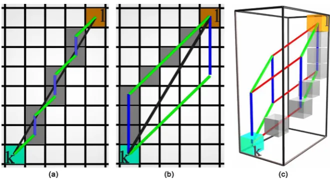
,k . The asymmetry of this measure proves useful in determining the LOS condition. Figure 1 illu-strates how the distance is asymmetric with regard to the path taken. Three con-ditions must be met if two partitions are LOS:1) A path must exist between
[ ]
k, that does not exit the convex hull, re-quiring L2 L2= T.2) The path found must take a direct path between
[ ]
k, , requiring that≤ T
L1 L1
Σ Σ .
3) The path found must follow the direct path, requiring ΣL1VAR≤
(
PC 2)
2.Dijkstra’s algorithm finds the minimal path taken between two points on a grid given an adjacency matrix, NN1, giving the path length,
L2
. Figure 1 il-lustrates that multiple paths have the same value forL2
, forming a parallelo-tope of possible paths each with the same minimal value. The true path length can be found simply by summing NN1 steps along the edge of the parallelo-tope, giving L2T. IfL2
exceeds L2T, the path found by Dijkstra has left the convex hull, leading to the first criteria. [image:7.595.207.538.409.589.2]To find the pathwise
Σ
L1
value, the adjacency matrix is altered, taking the row fromL1
for the kth partition and multiplying by every row of the logical matrix, NN1>0; in this way, the adjacency matrix presented to Dijkstra’sFigure 1. Illustrating various paths from the kth partition (cyan) to the ℓth (orange). Panel
DOI: 10.4236/jdaip.2018.63007 100 Journal of Data Analysis and Information Processing algorithm in a second round finds the minimal pathwise value from
[ ]
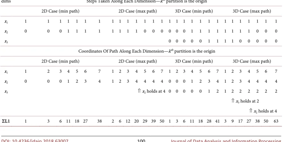
k, . For an open region (no obstacles), the minimal summed L1, ΣL1min, path is along the edge of the parallelotope.Table 1 shows the calculation of
Σ
L1
for both the minimal value as well as the maximal value from[ ]
k, , explaining whyΣ
L1
is asymmetric. Theexam-ple shown assumes that all paths between
[ ]
k, are possible, i.e. there are no obstructions. From the table, the sum of L1 steps is easier to calculate when viewed along each dimension. The minimal path takes the smallest size steps first, then increasing in size until the final partition is reached. In this manner, the sum of steps along each dimension is simply the summation of 1(
1)
2n n+
for each dimension along the convex hull. When traversing the maximal path, the largest steps are taken first, proceeding to the smallest steps taken last. In this case, a similar summation occurs, however, an additional amount for each di-mension is added because the path starts farther away from the initial point, which then adds successively along the path. The
Σ
L1
matrix will beasymme-tric as the minimal path from
[ ]
k, will not be the same from[ ]
,k . When following the minimal path according to Dijkstra from[ ]
,k , the path found follows the far opposite edge of the parallelotope, which is equivalent to the maximalΣ
L1
from[ ]
k, . The two extrema of the parallelotope between[ ]
k, represent the farthest paths that can be taken within the convex hull while always moving closer to the endpoint. The average between the two values ofmin
L1
Σ and ΣL1max is the true path ΣL1T.
When sufficient obstacles force the paths from
[ ]
k, as well as[ ]
,k to beTable 1. Table of steps, coordinates and the distance given by the summed L1 path, ΣL1, for the two examples in Figure 1(b), Figure 1(c). The top three rows represent the number of steps taken along each dimension from one partition to the next. The next three rows are the coordinates of the partitions along the paths taken, remembering that the path starts with the kth partition
at the origin. The final row is the summed L1 path distance. The axes are labeled where xi is from the longest dimension to the shortest of the convex hull.
dims Steps Taken Along Each Dimension—kth partition is the origin
2D Case (min path) 2D Case (max path) 3D Case (min path) 3D Case (max path) x1 1 1 1 1 1 1 1 1 1 1 1 1 1 1 1 1 1 1 1 1 1 1 1 1 1 1 1 1 x2 0 0 0 1 1 1 1 1 1 1 1 0 0 0 0 0 0 1 1 1 1 1 1 1 1 0 0 0
x3 0 0 0 0 0 1 1 1 1 0 0 0 0 0
Coordinates Of Path Along Each Dimension—kth partition is the origin
2D Case (min path) 2D Case (max path) 3D Case (min path) 3D Case (max path) x1 1 2 3 4 5 6 7 1 2 3 4 5 6 7 1 2 3 4 5 6 7 1 2 3 4 5 6 7 x2 0 0 0 1 2 3 4 1 2 3 4 4 4 4 0 0 0 1 2 3 4 1 2 3 4 4 4 4
x3 ⇑ x2 holds at 4 0 0 0 0 0 1 2 1 2 2 2 2 2 2
⇑ x3 holds at 2
⇑ x2 holds at 4
DOI: 10.4236/jdaip.2018.63007 101 Journal of Data Analysis and Information Processing along the same side of the parallelotope with respect to the true path, the path found “turns a corner” in order to reach the final partition. In this case, one of the two values, ΣL1k, or ΣL1,k will exceed the true path summed L1, ΣL1T,
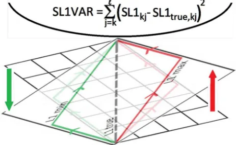
leading to the second criteria. The last criteria uses the results from the second application of Dijkstra, now, attempting to find a path that minimizes the va-riance of
Σ
L1
with respect to ΣL1T. Calculating the value(
)
2
− T
L1 L1
Σ Σ
then copying the kth row of this matrix and multiplying it by every row of the logical matrix, NN1>0, a new adjacency matrix is formed and applied using Dijkstra’s algorithm for the third time. At each step, the minimal summed path variance gives the most direct path from
[ ]
k, , finally giving the path that is LOS between the two partitions, illustrated in Figure 2. The smallest error that can exist is when a path is found that is one step off of the true path near the middle of the path. In this case, the error is the difference between 1(
1)
2n n+
and 1
(
1)( )
2 n− n , where n=PC 2, leading to the third criteria for LOS.
6. Strategy
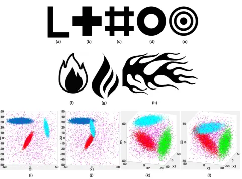
[image:9.595.256.488.471.614.2]This study employs 26 different clustering techniques to a bank of 12 representa-tive test cases. The data sets forming the test bank were comprised of various shapes, both connected and disconnected as well as point clouds in both 2D and 3D. In each of the point clouds, four gaussian distributions were placed near one another, with three densely populated regions and a fourth low density gaussian which spans the domain. The point clouds were further varied by creating one case in 2D and 3D where the dense gaussians are clearly separated, and another two cases in 2D and 3D where the three gaussians overlap. Figure 3 illustrates
Figure 2. Figure illustrates the two paths of ΣL1min and ΣL1max, which in 2D lie within
a plane. The average between them gives the straight line “true” value, ΣL1T. When all
paths within the L2 convex hull are available, Dijkstra’s algorithm will seek the ΣL1min
path when going from
[ ]
k, and will seek the ΣL1max path going from[ ]
,k . ThisDOI: 10.4236/jdaip.2018.63007 102 Journal of Data Analysis and Information Processing Figure 3. Test bank of 12 shapes: L (a), Plus-1 (b), Plus-2 (c), Concentric-1 (d), Concentric-2 (e), Flame-1 (f), Flame-2 (g), Flame-3 (h), Data2D-1 (i), Data2D-2 (j), Data3D-1 (k) and Data3D-2 (l).
DOI: 10.4236/jdaip.2018.63007 103 Journal of Data Analysis and Information Processing Table 2. Test bank data sets listing sizes and features relevant to clustering types.
Labels ID Test Bank Data Sets
Dim Size (pixels/pts) Connected Symmetry Plateau Filamentary Overlap Noise
L (a) 2D 1200 × 1200 √ X √ X X X
Plus1 (b) 2D 1200 × 1200 √ √ √ X X X
Plus2 (c) 2D 1200 × 1200 √ √ √ X X X
Concentric1 (d) 2D 1200 × 1200 √ √ √ X X X
Concentric2 (e) 2D 1200 × 1200 X √ √ X X X
Flame1 (f) 2D 1200 × 1200 √ X √ √ X X
Flame2 (g) 2D 1200 × 1200 X X √ X X X
Flame3 (h) 2D 1200 × 1200 √ X √ √ X X
Data2D-1 (pt. cloud) (i) 2D 200,000 X X X √ X √
Data2D-2 (pt. cloud) (j) 2D 200,000 √ X X √ √ √
Data3D-1 (pt. cloud) (k) 3D 200,000 X X X √ X √
Data3D-2 (pt. cloud) (l) 3D 200,000 √ X X √ √ √
overlap. For all cases other than the point clouds, the data is derived from an image, where a binary set of points is established for all 8-bit grey-scale values above 100 (1) or below (0). The image sizes when possible are 1200 × 1200, un-less the aspect ratio prevented that exact size. The point clouds are based on four distributions with a summed value of 200,000 points.
Along with the 26 clustering algorithms applied, four additional cluster as-signments are derived from consensus among the 26, leading to 30 differing cluster assignments per test case for a total of 360 figures showing the clustering results. These results are supplied as supplemental figures and can be found on the website. A sampling of these results is shown in Section 8.
7. Clustering Algorithms
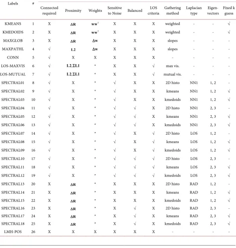
DOI: 10.4236/jdaip.2018.63007 104 Journal of Data Analysis and Information Processing Table 3 lists the twenty-six techniques used. Each technique attempts to cluster data according to features present in the data. The table lists those features which
Table 3. Clustering techniques for 26 algorithms highlighting requirements, pros and cons in each case. Some algorithms required partitions to be connected in order to search for clustering within the connected region. Clusters can be feature driven or can even the distribution of cluster assignments (balanced, group). LOS is a criterion for some clustering, which in turn can help identify data distributions. Finally, some algorithms treat isolated partitions on equal footing with larger connected subsets, making the clustering sensitive to these smaller subsets, interpreted as noise. Checks indicate a feature is used, “X” indicates the feature is not required whereas a “-” indicates the parameter is not applicable to the technique, finally “*” indicates that population weighting could be applied to the technique or not—for the results shown in this study, weights were applied to spectral algorithms making the Laplacian sensitive to the populations of the partitions.
Labels #
Clustering Algorithms
Connected
required Proximity Weights Sensitive to Noise Balanced criteria LOS Gathering method Laplacian type vectors Eigen- Fixed k guess
KMEANS 1 X ∆R wwΤ X X X weighted - - √
KMEDOIDS 2 X ∆R wwΤ X X X weighted - - √
MAXGLOB 3 X ∆R ∆w X X X slopes - - -
MAXPATHL 4 √ L2 ∆w X X X slopes - - -
CONN 5 √ X X X X X - - - -
LOS-MAXVIS 6 √ L2 L1,Σ * X X √ max vis. - - -
LOS-MUTUAL 7 √ L2 L1,Σ * X X √ mutual vis. - - -
SPECTRAL01 8 √ X * √ X X 2D histo NN1 1, 2 -
SPECTRAL02 9 √ X * √ X X kmeans NN1 1, 2 √
SPECTRAL03 10 √ X * √ X X kmedoids NN1 1, 2 √
SPECTRAL04 11 √ X * √ √ X 2D histo NN1 2, 3 -
SPECTRAL05 12 √ X * √ √ X kmeans NN1 2, 3 √
SPECTRAL06 13 √ X * √ √ X kmedoids NN1 2, 3 √
SPECTRAL07 14 √ X * √ X √ 2D histo LOS 1, 2 -
SPECTRAL08 15 √ X * √ X √ kmeans LOS 1, 2 √
SPECTRAL09 16 √ X * √ X √ kmedoids LOS 1, 2 √
SPECTRAL10 17 √ X * √ √ √ 2D histo LOS 2, 3 -
SPECTRAL11 18 √ X * √ √ √ kmeans LOS 2, 3 √
SPECTRAL12 19 √ X * √ √ √ kmedoids LOS 2, 3 √
SPECTRAL13 20 X ∆R * X X X 2D histo RAD 1, 2 -
SPECTRAL14 21 X ∆R * X X X kmeans RAD 1, 2 √
SPECTRAL15 22 X ∆R * X X X kmedoids RAD 1, 2 √
SPECTRAL16 23 X ∆R * X √ X 2D histo RAD 2, 3 -
SPECTRAL17 24 X ∆R * X √ X kmeans RAD 2, 3 √
SPECTRAL18 25 X ∆R * X √ X kmedoids RAD 2, 3 √
DOI: 10.4236/jdaip.2018.63007 105 Journal of Data Analysis and Information Processing best suit each technique. As the chief data reduction scheme here is to partition the data into multi-dimensional bins, the clustering is performed over the weighted partitions on a grid. Features indicated in the table are; require parti-tions to be Connected in order to cluster, Proximity uses distance as a criteria, Weights indicates populations affect the result, Sensitivity to Noise indicates some methods fail to find structure within larger connected subsets in the presence of noisy data, Balanced indicates methods which evenly divide parti-tions into clusters, LOS criteria is required for some, Gathering indicates the method used to gather partitions for clustering, Laplacian indicates which type of Laplacian is used for spectral algorithms, Eigenvectors indicate which mod-es are used in gathering, and Fixed k requires an initial guess as to the number of clusters.
7.1. K-Means and K-Medoids Clustering—KMEANS, KMEDOIDS
K-means is a well established clustering technique [10] [11], seeking from a data set, the lowest possible distance from individual data to a set of possible mean positions of the data, indicative of clusters. Over several passes, the cluster defini-tions are altered to minimize the distance from each datum to clusters found. An initial guess of the number of clusters to seek is required. K-means has been dis-cussed thoroughly in the community for its strengths and weaknesses [1]. K-medoids has been proposed to overcome many of the shortcomings of k-means and is similarly well-established in the community [5]. In both cases, an initial guess (k) as to the number of clusters sought is required which can be problematic when the actual number of clusters does not match the guessed val-ue. Further, both techniques perform at
( )
ND , which for large datasets arecostly. Progress in improvements to speed have been made to both techniques [12] [13], yet remain costly in high dimensions for large data sets. By shifting the analysis from individual datum to partitions with weights, the k-means and k-medoids algorithms are adjusted to accommodate the weighted bins. All calculations for distance between two partitions are multiplied by the weight of each partition, wwΤ, and any centroid calculation is treated as a weighted value.
7.2. Maxima Clustering—Global and Path Length
In this study, data has been reduced to a set of partitions with a population as-signed for each. The two schemes, MAXGLOB and MAXPATHL, assign data to clusters based on how close a partition is to a significant nearby maxima among the partitions. Treating the weights of the partitions as the height of a mul-ti-dimensional map, the significance of a nearby maxima is determined by cal-culating the slopes between any two partitions, where the slope is the ratio of the weight difference, ∆w, to the distance between any two partitions. In the global
case, the distance used is the Euclidean distance,
∆
R
, and for the path lengthDOI: 10.4236/jdaip.2018.63007 106 Journal of Data Analysis and Information Processing between partitions that are not required to be connected, while MAXPATHL requires a connection. Initially, local maxima among the partitions are found which are then categorized into three types: lone peaks, ridges and plateaus. Once the maxima are classified, a peak and all of the partitions associated with it are then assigned a cluster identification number, where the slopes and distances from partition to peak are contributing factors in determining which peaks asso-ciate with partitions. Definitions of local maxima, peaks and slopes as well as details of the algorithms for these two techniques are included in the supple-mental material online.
7.3. Clustering via Connection—CONN
In cases where local clusters of partitions are sparsely found within the data space, a simple clustering algorithm is to determine which partitions are con-nected to one another using first nearest neighbor steps, NN1. Section 4 dis-cusses path lengths calculated from one partition to another where those with a finite value are connected. A logical value is set between any two connected par-titions creating the matrix CONN. A unique cluster ID is assigned for each connected set of partitions.
7.4. Clustering by Line-of-Sight—LOS
Clustering by Line-of-Sight is motivated by the idea that two data within a con-vex region of a subset of the data have a higher chance of being correlated than data outside that convex region. Considering a set of data comprised of various types of distributions, it is possible for overlapping regions to form, where the tail of one distribution mingles with the tail of another. In the worst case scena-rio, peaks of two differing distributions may overlap. Further, distributions may also form along curved paths, where the peak may be far from the tails. Cluster-ing via CONN will associate all data in these distributions, however, checkCluster-ing whether two data lie within a convex hull more closely associates those data with one another. The Line-of-Sight criterion from Section 5 determines which parti-tions are convex to one another. As examples, Figures 3(i)-3(l) illustrate several distributions which have both convex regions as well as overlapping tails of dis-tributions. In this discussion, the term visibility refers to the number of parti-tions that are LOS to a specific partition. A detailed discussion of the algorithms used to form clusters based on the LOS criteria is provided by the supplemental material online.
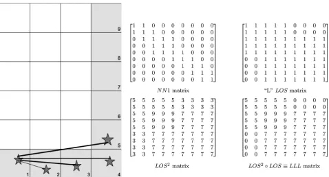
DOI: 10.4236/jdaip.2018.63007 107 Journal of Data Analysis and Information Processing that are not present in the LOS matrix, a Hadamard product is taken between LOS and LOS2 yielding a third matrix, LLL. To form clusters from the informa-tion in LLL, a gathering process finds partiinforma-tions that meet one of two cluster cri-teria; maximal visibility finds those partitions that share a high value of visibility and are connected to one another, and greatest mutual visibility finds the largest sets of partitions with a common value, regardless of how high in value is their visibility.
7.5. Simple Example: L
[image:15.595.59.538.380.638.2]A simple example serves to demonstrate how these matrices interact with one another. Consider a small distribution of partitions forming a 6 × 4 grid connected to each other in an “L” configuration as shown in Figure 4. The serialization of partitions is given by the same expression as the data, Equation (1), which in the case of the inverted L gives the partitions along the bottom row k=1 4 , then along the vertical side k=5 9 . In this case, there are only nine partitions con-nected to each other, requiring a 9 × 9 matrix to represent the information. As each partition is connected to all of the other partitions, the CONN matrix is full, with values of one. The NN1 matrix reflects which partitions share a common geometrical feature. The LOS, LOS2 and LLL matrices show which partitions are visible to each other. Note that partition five is visible to partition one, meaning
DOI: 10.4236/jdaip.2018.63007 108 Journal of Data Analysis and Information Processing that partitions can see the edges of one another. From the matrices shown, parti-tions (3, 4, 5) form a cluster with the maximal visibility, followed by partiparti-tions (6, 7, 8, 9) then (1, 2) (LOS-MAXVIS). Partitions (3, 4, 5, 6, 7, 8, 9) form a cluster with the highest mutual visibility followed by (1, 2) with the lowest (LOS-MUTUAL).
7.5.1. LOS Clustering with Maximal Visibility—LOS-MAXVIS
The LOS matrix contains for each row the logical status of which partitions are LOS to the current partition. Further, the LLL matrix shows the number of mu-tually visible partitions within LOS of the current. From the LLL matrix, two values can be used to determine clustering using LOS. The highest value in the LLL matrix indicates which partitions are within LOS of the most other parti-tions. These highest valued LLL partitions have the maximal visibility, LOS-MAXVIS, of the set of partitions that are LOS. An example would be any partition that is located at an intersection of several distributions of partitions. Consider the test cases: L and Plus1, where the corner of the L and the center of the Plus1 will have maximal visibility. The clusters formed in this manner find intersections and corners of data distributions preferentially, leading to data identification of the entangled portions of data sets arising from multiple distri-butions present.
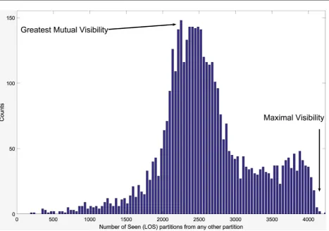
Clustering by LOS-MAXVIS is achieved by forming a histogram from the vi-sibility values of LLL, shown in Figure 5 for the Data3D2 test case. The horizon-al axis indicates the visibility while the vertichorizon-al axis is the number of partitions sharing a common visibility value. Starting from the maximal value of the visi-bility, a cluster is formed by taking all partitions sharing the maximum or nearby, defined by including all bins in the histogram starting from the leftmost until a minimum in the bins is reached. In the case of the simple L, the most visible par-titions are the corner parpar-titions with values LLL = 9. Of the set of parpar-titions found, a cluster is assigned to the largest connected group of partitions. As each cluster is identified, the partitions are excluded from further searches by remov-ing the rows and columns from LLL of the cluster found then recalculatremov-ing the histogram. Further clusters are then identified by taking partitions associated with the next highest visibility bin in the histogram, beginning where the last set left off, and including all partitions with successively lower visibilities until the next minimum in the bins is reached. This process continues until the set of par-titions is fully associated with clusters.
7.5.2. LOS Clustering with Mutual Visibility—LOS-MUTUAL
DOI: 10.4236/jdaip.2018.63007 109 Journal of Data Analysis and Information Processing Figure 5. Histogram of LLL values, the visibility from a partition to all others for the Data 3D-2 case. Along the horizontal axis are visibility values and along the vertical axis is the frequency of partitions for a given visibility. For the Data 3D-2 case, the highest visibility is ≈4100 between partitions, where LOS-MAXVIS begins searching at the highest visibility bin and ends at the first mi-nima found in the histogram, for a cluster with visibility from ≈ 3300 - 4100. A LOS-MUTUAL search seeks a cluster with the greatest mutual visibility by beginning the search at the tallest peak around ≈2200 whose set size is ≈150 partitions. The cluster is formed between the two minima found on each side of the tallest peak. In both cases, the starting point for the cluster search de-fines which other partitions are near to the goal, either maximal visibility or greatest mutual visibility. The clusters are formed by grouping LOS partitions around the feature sought in the histogram, where peaks are separated by the basins.
found, all partitions which have any visibility values in LLL within this range are clustered together. Identifies partitions are removed from further searches and the process is repeated until all partitions are identified. LOS-MUTUAL cluster-ing finds the largest set of partitions that are LOS to each other first, then searches for the next largest set of partitions that do not include the first set and so on. In the case of the simple L, the highest mutually visible partitions are the partitions forming the long arm of the L, with values LLL = 7. For the Data3D2 case, all partitions with a visibility between 1700 up to 3000 are included in the first cluster found. As before, once a cluster is found, the partitions are removed from further searches. Clusters formed in this manner find full data distributions first, associating tails over mixed regions with the largest distributions first, giv-ing an alternative to the data identification offered by LOS-MAXVIS.
7.6. Spectral Clustering
ver-DOI: 10.4236/jdaip.2018.63007 110 Journal of Data Analysis and Information Processing tices and relationships between data points are represented by edges and weights in the graph. The eigenmodes of the graph are sought solving Helmholtz equa-tion from a Laplacian chosen based on the edge weights. This analysis uses the NN1 matrix, the LOS matrix as well as a radial basis function to form the graphs. The Laplacian operator is a matrix formed by setting the degree of the vertex along the diagonal with off diagonal elements set to a negative weight factor. The off diagonal components are formed from either the summation of all nearest neighbors (NN1), the sum of all LOS partitions (LOS) or a radial factor related to the distance squared to all other partitions (RAD). RAD is chosen as a gaus-sian with a large sigma equal to the maximal distance of
∆
R
. Clustering with NN1 seeks clusters as partitions connected to one another, using LOS seeks similar clustering for partitions connected through visibility, while RAD seeks clusters of partitions over a region, regardless of connection. In all cases, the analysis that follows is similar. The eigenvectors are calculated for the Lapla-cian, where the lowest two eigenvectors are typically used to define a new data space using each eigenvector as a basis. The partitions are then mapped to the eigenspace and clusters within the space are sought using novel 2D clustering techniques, either KMEANS, KMEDOIDS or a simple 2D histogram over the domain.This analysis employs all three clustering techniques in the eigenspace as well as explores using two differing sets of eigenvectors, the lowest pair (1, 2) as well as the next lowest pair (2, 3) as a base. Spectral clustering finds clusters of partitions which are connected subdomains; however, when only a single connected domain is found (clean case), the eigenvectors reveal a modal structure within the connected domain. When showing the modal structure for the first case using eigenvectors (1, 2), the first eigenmode accentuates a single large feature within the eigenspace, where the second eigenvector seg-ments the space into a small number of symmetric regions. When using the next lowest pair of eigenvectors (2, 3), surpassing the lowest eigenmode, the modal structure segregates the partitions differently, clustering the partitions into evenly distributed groups of data. Once the eigenspace has been populated with the partitions, k-means, k-medoids as well as traditional 2D histograms can be used to collect the partitions and assign them to cluster IDs. K-means and k-medoids have been discussed earlier in Sec. 1 as to their strengths and weaknesses. As an alternative approach to finding the clusters within the ei-genspace, simply histogram the 2D eigenspace and assign to each non-zero bin a different cluster ID (2DHIST). This approach has the advantage of simplicity and finds exactly the number of clusters that fill bins within the eigenspace, not requiring an initial guess as the number of possible clusters, as in the case of k-means or k-medoids, however a maximum possible count of clusters is set by the number of bins of the 2D histogram, typically set at
(
k+ ×2) (
k+2)
DOI: 10.4236/jdaip.2018.63007 111 Journal of Data Analysis and Information Processing
7.7. Clustering by Coarse Position (LMH-POS)
The most obvious form of clustering is to associate a partition solely by its posi-tion (LMH-POS) using a coarse binning within the partition space. By setting the number of bins along each dimension to three, the bins are interpreted as being Low, Medium or High for the values represented along each axis. In this case, the sequential partition bin index, k, becomes the cluster ID, with the maximum number of possible clusters at 3ND, for the three bins along each axis.
This approach is a coarse designation for clustering as it employs no compli-cated algorithms, and data with similar values are associated irrespective of all other factors. This approach suffers from many problems in that data in one bin will not be clustered with data from a neighboring bin no matter how close in proximity the two are to one another. Clusters from LMH-POS characterize data in the crudest sense with no refinement for the shape of a distribution or even the relative sizes of the distribution. One advantage to this approach is that it is easy to understand, even while spanning multiple dimensions, making it an easy entry point for a discussion of the data. When handling large data sets, this approach allows for a quick look at where the data reside within the larger space.
8. Results
This section shows a sampling of results from the application of 26 techniques to 12 test cases. The strengths and weaknesses of these techniques are exposed leading to the conclusion that a consensus approach is reasonable. Ideally, all clustering techniques plus the four robust consensus results of each test case would be presented, leading to 360 figures, but due to space limitations, the full set of clustering results are provided in the supplemental material. Throughout this section, the term “noise” refers to data sets where a significant number of isolated small subsets of partitions, including singletons, are present, while the term “clean” refers to data sets without these smaller subsets. Among the sup-plemental material, for each data set, a high data threshold, Θperc=2%, and a
low threshold, Θperc=0%, are applied showing how clustering is achieved in a
clean versus noisy environment respectively. Data clustering is also shown at two different bin resolutions to illustrate how too fine of a resolution may not achieve good clustering. Finally, the figures are grouped into fullpage compari-sons for a single test case with all 30 techniques shown as well as single page comparison for each technique across all test cases, leading to 2880 figures over 168 pages.
8.1. Discussion of Techniques
remain-DOI: 10.4236/jdaip.2018.63007 112 Journal of Data Analysis and Information Processing ing figures are chosen to demonstrate a particular trait of a clustering technique. Figure 12 shows all of the techniques applied to the Data2d2 test case. When appropriate, a circle is shown within a cluster to indicate the medoid of the clus-ter.
K-means and k-medoids results are well understood for both their strengths and weaknesses. MAXGLOB and MAXPATHL tend to mirror results from k-means and k-medoids with the exception that MAXPATHL is restricted to clustering within a connected set, making it seek clusters following a distributions’ shapes rather than just using proximity between data. The CONN technique clusters data within a connected set regardless of other criteria. LOS-MAXVIS and LOS-MUTUAL cluster according to data within convex hulls, seeking similar vi-sibility features as part of the gathering criteria to form clusters. Spectral tech-niques form clusters within the eigenspace formed from two eigenvectors. The adjacency matrix used to form the Laplacian determines the nature of the neighbors used, traditionally a first nearest neighbor, however, this study em-ploys both the LOS criteria to define “neighbors” as well as a radial basis. Fur-ther, the choice of eigenvectors used to form the eigenspace determines whether a prominent feature is clustered about (using the 1st and 2nd eigenvectors), or a more evenly distributed clustering is achieved using the 2nd and 3rd eigenvec-tors. Due to the number of variations in spectral clustering, the techniques are identified by an index given in Table 3, while in the text, a shorthand will be used: ([1][2], NN1, 2DHIST) to represent the use of the 1st and 2nd eigenvec-tors, utilizing a Laplacian based on an adjacency matrix derived from the first nearest neighbor matrix NN1 and gathering the partitions into clusters within the eigenspace using a 2D histogram (6 × 6) bins. Other variations in the nota-tion are: [2] [3] for eigenvectors, LOS or RAD for the adjacency matrix, and “kmeans” or “kmedoids” to be used in the gathering of partitions within the ei-genspace. Finally, the LMH-POS technique clusters using a course resolution (Low-Medium-High valued) for the binning choice, simply separating the do-main into three bins per dimension to get a quick look at how the data is distri-buted.
Figures 6-8 show the clustering results for the data sets derived from images, where one datum exists for each pixel turned on. After binning, these test cases generally have flat distributions, so the clustering results reflect geometrical fea-tures, useful for showing data grouping. Figures 9-12 show the clustering results for simulated data sets for ellipsoidal distributions, where the data is unevenly distributed, some with overlapping tails, helpful in illustrating data identifica-tion.
8.2. Concentric1
in-DOI: 10.4236/jdaip.2018.63007 113 Journal of Data Analysis and Information Processing to two groups, those that adhere to the symmetry of the domain and those that break the symmetry. K-medoids (6a) shows the attempt of creating 16 clusters that almost respect the symmetry of the data set. LOS-MAXVIS (6b) finds clus-ters based on highest visibility first, where it assigns clusclus-ters to a set of three subsets first, then proceeds to find further clusters within the remaining set of data, creating an odd symmetry around the ring. LOS-MUTUAL (6c) finds clus-ters based on the largest set of partitions with visibility values in common, lead-ing to one large cluster formed, then the next largest, and so on until all data are clustered, making this a “greedy” algorithm, taking the largest pieces first. SPECTRAL01 (6d) finds clusters ([1][2], NN1, 2DHIST), which finds a single large subset of the data first based on modes, then proceeds to cluster to smaller subsets. This approach has the effect of creating clusters that “stripe” the domain starting from the large feature to the smaller features. SPECTRAL06 (6e) clusters ([2] [3], NN1, kmedoids) balance the assignment of clusters to data, creating more evenly spaced clusters. SPECTRAL07 (6f) clusters ([1][2], LOS, 2DHIST) have the effect of finding large features based on visibility first, then smaller visi-bility clusters next. SPECTRAL12 (6g) clusters ([2] [3], LOS, kmedoids) at-tempts to balance the LOS assignments. SPECTRAL15 (6h) finds clusters ([1][2], RAD, kmedoids) Laplacian based on a gaussian to assign clusters, leading to a set of clusters formed around a central location—in this case, the center of the ring.
8.3. L and Plus1
DOI: 10.4236/jdaip.2018.63007 114 Journal of Data Analysis and Information Processing Figure 6. Test bank case for Concentric1 showing the following techniques: (a) KMEDOIDS (k = 16); (b) LOS-MAXVIS; (c) LOS-MUTUAL; (d) SPECTRAL01; (e) SPECTRAL06; (f) SPECTRAL07; (g) SPECTRAL12; (h) SPECTRAL15.
[image:22.595.59.545.373.682.2]DOI: 10.4236/jdaip.2018.63007 115 Journal of Data Analysis and Information Processing
8.4.
Flame
1 and
Flame
3
Figure 8 shows clustering for the Flame1 and Flame3 cases, where symmetry is not present yet filamentary features are present with both close and larger gaps as well. K-medoids are shown first in both cases (8a, 8e) showing typical clus-tering based on proximity, worth noting is that when gaps become close, k-medoids will create a single cluster on both sides of the gap due to proximity. For Flame1, LOS-MUTUAL (8b) finds clusters in subsets grouped by visibility, finding the most in common first. The large group of small clusters can be as-signed to nearby larger clusters, however, this study did not focus on this level of refinement, mainly the viability of the algorithm to seek clusters. SPECTRAL12 (8c) clusters ([2] [3], LOS, kmedoids) using visibility as well finding similar groups with small deviations. SPECTRAL15 (8d) clusters ([1][2], NN1, kmedo-ids) using a radial basis clustering around a central location in the middle of the flame. For Flame3, LOS-MAXVIS (8f) finds clusters according to maximal visi-bility first exposing long clusters within the filamentary portions of the flame. SPECTRAL06 (8g) clusters ([1][2], NN1, kmedoids) larger features first irres-pective of gaps in the data, striping to smaller to features.
8.5. Data2D-1
DOI: 10.4236/jdaip.2018.63007 116 Journal of Data Analysis and Information Processing Figure 8. Test bank case for Flame1 showing the following techniques: (a) KMEDOIDS (k = 16); (b) LOS-MUTUAL; (c) SPECTRAL12; (d) SPECTRAL15. Test bank case for Flame3 showing the following techniques: (e) KMEDOIDS (k = 16); (f) LOS-MAXVIS; (g) SPECTRAL06.
[image:24.595.59.542.411.680.2]DOI: 10.4236/jdaip.2018.63007 117 Journal of Data Analysis and Information Processing number of non-zero elements, favoring the larger clusters first. SPECTRAL07 (9g) clusters ([1] [2], LOS, 2DHIST) identifies the three large ellipsoids more consistently than SPECTRAL02, among the large set of singleton partitions. SPECTRAL15 (9h) clustering ([1][2], RAD, kmedoids) is less sensitive to sin-gleton and small subsets as the adjacency matrix correlates partitions from dis-connected regions, such the clusters formed are showing the modal structure rather than the connected structure.
8.6. Data3D-1
Figure 10 shows clustering for the Data3D-1 case, where little symmetry is present in a clean environment at a high bin resolution where no distributions overlap. K-medoids (10a) shows 16 clusters found in three main ellipsoids, with k-means (10b) giving similar yet different results. CONN (10c) clusters parti-tions connected to one another, which in a clean environment finds three ellip-soidal distributions, however, some partitions may have been “cutoff” from the main ellipsoids due to the higher data threshold placed, leading to singleton clusters. MAXPATHL (10d) shows similar results to CONN, however, additional clusters are found due to local maxima in the weighted partitions, leading to smaller clusters near the edge of the subsets along with the three main ellipsoids. LOS-MAXVIS (10e) clusters by maximal visibility first, finding variation within the three main ellipsoids based on visibility. SPECTRAL01 (10f) ([1][2], NN1, 2DHIST) again finds difficulty finding the three ellipsoids in the presence of noise, whereas SPECTRAL07 (10g) ([1] [2], LOS, 2DHIST) under the same conditions finds the three clusters. ROBUST2 (10h) clusters according to a consensus of 50% of the algorithms in agreement of cluster IDs.
8.7. Data3D-2
DOI: 10.4236/jdaip.2018.63007 118 Journal of Data Analysis and Information Processing Figure 10. Test bank case for Data3D1 in a low noise environment, Θperc =2%, showing the following techniques: (a) KMEDOIDS (k = 16); (b) KMEANS (k = 16); (c) CONN; (d) MAXPATHL; (e) LOS-MAXVIS; (f) SPECTRAL01; (g) SPECTRAL07; (h) ROBUST2.
[image:26.595.58.543.407.678.2]DOI: 10.4236/jdaip.2018.63007 119 Journal of Data Analysis and Information Processing
8.8. Data2D-2
Figure 12 shows clustering for the Data2D-2 case, where little symmetry is present in a noisy environment at a high bin resolution where three distributions overlap. All 26 techniques are on display allowing for a cross-comparison along with the four robust algorithms in the last row (slightly larger). Of the 26 algo-rithms, 14 have been discussed in the previous test cases. Among the spectral techniques in a noisy environment, SPECTRAL01-SPECRTAL12, when the number of clusters sought is less than the high multiplicity of the lowest eigen-value, without additionally specifying the order of the eigenvectors, the possibil-ity exists that some larger subsets of the data will not be clustered as expected, leading to smaller subsets assigned to clusters otherwise seen as noise (single-tons). The radial basis spectral techniques do not suffer from this confusion as they do not require a connection between the partitions in order to form clusters, allowing the approach to be sensitive to the larger structure within the domain, creating clusters around centroids within the data.
9. Robust Clustering over Multiple Algorithms
In this paper, multiple clustering algorithms have been presented and applied to several test cases. Each technique has strengths as well as weaknesses which have been exposed through the cases presented. When using multiple techniques, the possibility exists to leverage the information gathered from all techniques to ar-rive at a final cluster designation, based on the level of agreement or disagree-ment found between the algorithms [8]. This approach is comparable to ensem-ble modeling used in various fields [16] [17]. This section proposes four possible robust ways to gather the cluster information and assign new cluster IDs.
In each approach taken, the cluster information for the partitions is represented by a matrix of cluster IDs, where each row represents results from a single cluster algorithm and each column is a partition. The values along each row are the cluster IDs assigned to each partition, forming the matrix,
{
CLUS∈C P×}
where C = 26 and P is the number of partitions. In order toDOI: 10.4236/jdaip.2018.63007 121 Journal of Data Analysis and Information Processing Table 4. A sample set of partitions that have had six differing cluster algorithms applied. In each case, the cluster algorithm identi-fied up to nine different clusters. The set contains 40 partitions. The top table represents the data initially unsorted. Each row is a different cluster algorithm and each column is a partition where a cluster ID has been assigned. The second table has sorted each row while maintaining the assignments to each partition. The third table from the top shows the differences in cluster ID assign-ments from one column to the next. The fourth table is the final cluster assignment given to the partitions when any one change occurs (a disagreement) between the cluster algorithms. The fifth table requires a 50% majority of the cluster algorithms to change (cumulatively) before a new cluster assignment is designated. The sixth table only changes the cluster assignment once all cluster algorithms cumulatively have changed. Finally, the last table requires that all algorithms change assignments simultaneously be-fore a new cluster ID is designated (the clusters are disjoint—with no overlap).
40 Partition Cluster IDs
Alg1 5 7 2 4 7 1 2 4 1 1 2 3 8 6 4 1 5 5 4 1 1 4 8 8 9 6 9 4 1 2 4 4 4 1 7 4 3 3 4 Alg2 7 7 3 7 7 1 3 7 3 1 3 4 7 7 6 1 7 7 5 1 2 5 7 7 7 7 7 5 1 3 6 7 6 1 7 7 5 3 5 Alg3 6 6 2 6 7 1 3 6 2 1 3 3 8 6 5 1 6 6 5 1 1 5 8 8 8 6 8 5 1 2 5 6 6 1 6 6 3 3 5 Alg4 4 5 2 4 6 1 2 4 2 1 2 2 6 4 4 1 4 4 2 1 2 3 6 6 6 5 6 2 1 2 3 4 4 1 5 4 2 2 2 Alg5 5 6 1 4 6 1 1 5 1 1 1 2 6 6 4 1 6 5 3 1 1 4 6 6 6 6 6 4 1 1 4 4 4 1 6 4 2 1 4 Alg6 6 8 1 5 8 1 2 5 1 1 3 4 8 7 4 1 7 5 4 1 1 4 9 9 9 7 9 4 1 1 4 5 5 1 7 5 4 3 4
40 Partition Cluster IDs—Resorted by Partitions in Ascending ID Order
Alg5 1 1 1 1 1 1 1 1 1 1 1 1 1 2 2 3 3 4 4 4 4 4 4 4 4 4 5 5 5 6 6 6 6 6 6 6 6 6 6 Alg6 1 1 1 1 1 1 1 1 1 1 2 3 3 4 4 4 4 4 4 4 4 4 5 5 5 5 5 5 6 7 7 7 7 8 8 8 9 9 9 Alg1 1 1 1 1 1 1 1 1 2 2 2 2 3 3 3 3 4 4 4 4 4 4 4 4 4 4 4 5 5 5 6 6 7 7 7 8 8 8 9 Alg3 1 1 1 1 1 1 1 2 2 2 3 3 3 3 3 4 5 5 5 5 5 5 6 6 6 6 6 6 6 6 6 6 6 6 7 8 8 8 8 Alg4 1 1 1 1 1 1 2 2 2 2 2 2 2 2 2 2 2 2 2 3 3 4 4 4 4 4 4 4 4 4 4 5 5 5 6 6 6 6 6 Alg2 1 1 1 1 1 1 2 3 3 3 3 3 3 4 5 5 5 5 5 5 6 6 6 7 7 7 7 7 7 7 7 7 7 7 7 7 7 7 7
40 Partition Cluster Difference Flags (Logical) for Sorted IDs
Alg5 0 0 0 0 0 0 0 0 0 0 0 0 0 1 0 1 0 1 0 0 0 0 0 0 0 0 1 0 0 1 0 0 0 0 0 0 0 0 0 Alg6 0 0 0 0 0 0 0 0 0 0 1 1 0 1 0 0 0 0 0 0 0 0 1 0 0 0 0 0 1 1 0 0 0 1 0 0 1 0 0 Alg1 0 0 0 0 0 0 0 0 1 0 0 0 1 0 0 0 1 0 0 0 0 0 0 0 0 0 0 1 0 0 1 0 1 0 0 1 0 0 1 Alg3 0 0 0 0 0 0 0 1 0 0 1 0 0 0 0 1 1 0 0 0 0 0 1 0 0 0 0 0 0 0 0 0 0 0 1 1 0 0 0 Alg4 0 0 0 0 0 0 1 0 0 0 0 0 0 0 0 0 0 0 0 1 0 1 0 0 0 0 0 0 0 0 0 1 0 0 1 0 0 0 0 Alg2 0 0 0 0 0 0 1 1 0 0 0 0 0 1 1 0 0 0 0 0 1 0 0 1 0 0 0 0 0 0 0 0 0 0 0 0 0 0 0
40 Partition Cluster Fractured IDs
Rob1 1 1 1 1 1 1 2 3 4 4 5 6 7 8 9 10 11 12 12 13 14 15 16 17 17 17 18 19 20 21 22 23 24 25 26 27 28 28 29 40 Partition Cluster Majority Changed IDs
Rob2 1 1 1 1 1 1 1 2 2 2 3 3 3 4 4 5 5 6 6 6 6 6 7 7 7 7 7 8 8 8 9 9 9 10 10 11 11 11 11 40 Partition Cluster All Changed IDs
Rob3 1 1 1 1 1 1 1 1 1 1 1 1 1 2 2 2 2 2 2 2 2 2 3 3 3 3 3 3 3 3 3 3 3 3 4 4 4 4 4 40 Partition Cluster No Overlap IDs
DOI: 10.4236/jdaip.2018.63007 122 Journal of Data Analysis and Information Processing following the partitions from left to right across the page.
As examples of robust clustering, the last four figures from Figure 12 as well as Table 4 are provided to illustrate the process. These figures show the results from a consensus using all clustering techniques excluding the LMH-POS algo-rithm for the Data2D2 test case with no minimal population set for the parti-tions. The LMH-POS technique was excluded as its partition definitions do not align with the remaining 25 algorithms. In cases where multiple techniques are compared using differing partition sizes, the robust technique is then applied per datum, using the same procedures, however, the sorting is performed over all data instead of partitions. The last four figures from Figure 12 show the follow-ing consensus techniques, from left to right, the Fractured, Majority Changed (75%), All Changed (100%) and No Overlap cases.
The Fractured robust designation results by assigning each partition a new cluster ID starting from one and increasing the cluster ID each time any tech-nique changes its ID, which results in the largest set of clusters found. This approach is the most sensitive to changes in the cluster designations. The Ma-jority Changed robust technique assigns a new cluster ID each time the accu-mulated number of algorithm cluster ID changes reaches a majority of the to-tal number of algorithms. For each clustering technique, when a change occurs, any further changes from that technique are not registered until a majority is reached, at which point the accumulated sum of changes is reset to zero. This results in a medium sized set of clusters found, where a significant number of algorithms found a change, however, not all algorithms are required to note the change in ID. In the figure, a 75% majority was required, where ideally, the best majority threshold would create the largest number of clusters with the highest average membership. The All Changed robust case is equivalent to the Majority Changed case with a 100% majority threshold. This results in a small-medium sized set of clusters found, where every algorithm found a change, however, the changes may not have been at the same partition number, merely, that the total set of changes across all algorithms eventually required a change of ID. The No Overlap robust case assigns a new cluster ID whenever the total number of algorithms changes designation simultaneously, resulting in the smallest sized set of clusters found, where every algorithm must find a change for all partitions in a subset. Ideally, this would happen for each dis-connected group of partitions, however, several techniques are “global” in scope and do not require a connection to exist to form clusters, leading to a single large cluster.
DOI: 10.4236/jdaip.2018.63007 123 Journal of Data Analysis and Information Processing the number of clusters found can be used as a k-value, which allows a reasonable guess to re-run the analysis utilizing the full complement of techniques.
10. Conclusions
A study using 26 clustering techniques has been performed over 12 test cases to illustrate both the strengths and weaknesses of clustering algorithms. A robust form of clustering is achieved through consensus over all techniques, helping reduce clustering problems by finding consistent clustering definitions across many approaches. The approach taken by this study utilizes six main ideas to produce a robust clustering analysis:
• Reduce a large data set by binning the space, where the filled bins are the multi-dimensional partitions of the data set, each with a unique serial index, k.
• Algorithms use the path length between any connected partitions as well as traditional distance metrics (L1, L2, etc.).
• A Line-of-Sight (LOS) algorithm is developed to enhance the probability that two data are associated with one another. LOS also provides a new “super” neighborhood definition to be used in graph-based techniques. Data identi-fication is addressed in two differing ways by LOS.
• Spectral clustering using the [2] [3] eigenvectors addresses data grouping better than other methods.
• Employ multiple clustering techniques to the set of partitions based on first nearest neighbors, distance weighted factors and geometrical properties of the set.
• Using a consensus overcomes any one techniques’ failure mode in favor of the strengths of multiple techniques.
• Establish a final cluster ID based on all the consensus of techniques em-ployed.
This study shows that high dimensional, big-data analysis can be reduced to a smaller set of partitions where multiple clustering techniques can be used to sort the data into clusters. While the techniques presented are all computationally
( )
2P N
, by reducing the data set to partitions, these routines are reasonable to perform. The introduction of the LOS criteria created new avenues for cluster seeking. The combination of multiple clustering techniques, various distance metrics and traditional data reduction leads to a robust set of clusters found, which worked well in addressing issues of data identification, clustering as well as grouping.