Western University Western University
Scholarship@Western
Scholarship@Western
Electronic Thesis and Dissertation Repository
11-29-2016 12:00 AM
Improved Localization Algorithms in Indoor Wireless Environment
Improved Localization Algorithms in Indoor Wireless Environment
Fei Long
The University of Western Ontario
Supervisor Dr. Xianbin Wang
The University of Western Ontario Joint Supervisor Dr. Jagath Samarabandu
The University of Western Ontario
Graduate Program in Electrical and Computer Engineering
A thesis submitted in partial fulfillment of the requirements for the degree in Master of Engineering Science
© Fei Long 2016
Follow this and additional works at: https://ir.lib.uwo.ca/etd
Part of the Systems and Communications Commons
Recommended Citation Recommended Citation
Long, Fei, "Improved Localization Algorithms in Indoor Wireless Environment" (2016). Electronic Thesis and Dissertation Repository. 4284.
https://ir.lib.uwo.ca/etd/4284
This Dissertation/Thesis is brought to you for free and open access by Scholarship@Western. It has been accepted for inclusion in Electronic Thesis and Dissertation Repository by an authorized administrator of
Localization has been considered as an important precondition for the location-dependent
applications such as mobile tracking and navigation.To obtain specific location information,
we usually make use of Global Positioning System(GPS), which is the most common
plat-form to acquire localization inplat-formation in outdoor environments. When targets are in indoor
environment, however, the GPS signal is usually blocked, so we also consider other assisted
po-sitioning techniques in order to obtain accurate position of targets. In this thesis, three different
schemes in indoor environment are proposed to minimize localization error by placing
refer-ence nodes in optimum locations, combining the localization information from accelerometer
sensor in smartphone with Received Signal Strength (RSS) from reference nodes, and utilizing
frequency diversity in Wireless Fidelity (WiFi) environment.
Deployments of reference nodes are vital for locating nearby targets since they are used to
estimate the distances from them to the targets. A reference nodes’ placement scheme based
on minimizing the average mean square error of localization over a certain region is proposed
in this thesis first and is applied in different localization regions which are circular, square and
hexagonal for illustration of the flexibility of the proposed scheme.
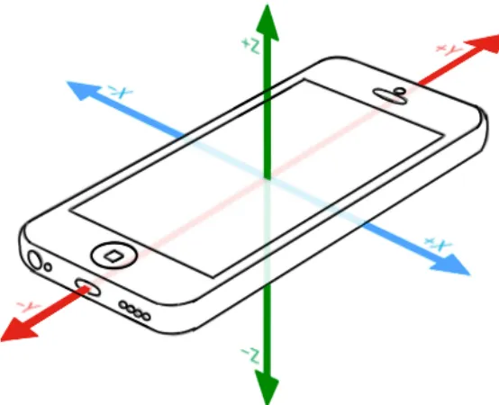
Equipped with accelerometer sensor, smartphone provides useful information which out-puts accelerations in three different directions. Combining acceleration information from
smart-phones and signal strength information from reference nodes to prevent the accumulated error
from accelerometer is studied in this thesis. The combined locating error is narrowed by
as-signing different weights to localization information from accelerometer and reference nodes.
In indoor environment, RSS technology based localization is the most common way to
imply since it require less additional hardware compared to other localization technologies.
However, RSS can be affected greatly by complex circumstance as well as carrier frequency.
Utilization of diverse frequencies to improve localization performance is proposed in the end
of this thesis along with some experiments applied on Software Defined Platform (SDR).
Acknowledgements
I would like to express my special appreciation and sincere thanks to my supervisor
Profes-sor Dr. Xianbin Wang, you have been a tremendous mentor for me. I would like thank you for
encouraging my research and for guiding me to complete this thesis. Your advice on both
re-search as well as on my career have been priceless. I also would like to thank my co-supervisor
Dr. Jagath Samarabandu for your help and advices during my graduate study period.
Besides my supervisors, I would like to thank the examiners from my thesis committee:
Dr. Raveendra Rao, Dr. Liying Jiang and Dr. Weiming Shen, for coming for my thesis defence
and helping me to improve my thesis quality.
I also would like to take this opportunity to express gratitude to all of the Department
faculty members for their help and support.
I would like to thank my colleague, Dr. Aydin Behnad, Yu He and Kejun Tong for their
help on my research.
Moreover, I would like to thank my research group, they not only give help on my research
but also on my daily life. They are not only my colleagues but also my friends. Thanks to you
guys for your support and accompany.
A special thanks to my family. Words can not express now grateful I am to my mother and
father for all of the sacrifices that you have done on my behalf. I would also like to thank all of
my friends who supported me in writing and encourage me to strive towards my goal.
Certificate of Examination ii
Abstract ii
List of Figures vii
List of Tables ix
1 Introduction 2
1.1 Motivation . . . 2
1.2 Research Objectives . . . 4
1.3 Contributions . . . 5
1.4 Thesis Outline . . . 6
2 Localization Techniques and Algorithms 7 2.1 Range Based Localization Technologies . . . 8
2.1.1 Signal Strength-Based Localization . . . 8
Signal fading in wireless communications . . . 9
Received Signal Strength Indicator technologies . . . 12
2.1.2 Time Based Localization . . . 14
2.1.3 Angle Based Localization . . . 15
2.2 Localization Estimation Algorithms . . . 16
2.2.1 Least square estimation . . . 16
2.2.2 Maximum likelihood estimation . . . 18
2.2.3 Cram´er-Rao Lower Bound . . . 20
2.3 Sensor Measurements . . . 22
2.3.1 Accelerometer . . . 22
2.3.2 Magnetometer . . . 23
2.3.3 Gyroscope . . . 23
2.4 Chapter Summary . . . 23
3 Optimum Reference Node Deployment for Indoor Localization Based on the Average Mean Square Error Minimization 25 3.1 Introduction . . . 25
3.2 Minimum Mean Square Error Scheme . . . 27
3.3 Average Scheme In Certain Localization Regions . . . 29
3.4 Simulation Results . . . 33
3.4.1 Circular Region . . . 33
3.4.2 Hexagonal Region . . . 35
3.4.3 Square Region . . . 37
3.5 Chapter Summary . . . 39
4 Joint Localization Algorithm Combining Information from Accelerometer and Available Reference Nodes 41 4.1 Introduction . . . 42
4.2 System Model . . . 44
4.2.1 Accelerometer based localization . . . 44
4.2.2 Accelerometer and available reference node combined localization al-gorithm . . . 46
4.2.3 Weighted assignments for accelerometer and reference nodes . . . 49
4.3 Simulation Results . . . 50
4.3.2 Smartphone-based measurement . . . 51
4.3.3 User trajectory simulation . . . 54
4.4 Chapter Conclusion . . . 57
5 Improving Log-distance Path Loss Localization Model by Utilizing Frequency Diversity 58 5.1 Introduction . . . 59
5.2 System Model . . . 60
5.2.1 Trilateration . . . 61
5.2.2 System model . . . 62
Frequency based path loss model . . . 62
Weighted algorithm . . . 64
5.3 Software Defined Radio Platform . . . 67
5.3.1 Gain control . . . 68
Transmit gain . . . 69
Receive gain . . . 69
5.3.2 Implement procedure . . . 69
5.4 Experimental Results . . . 72
5.5 Chapter Summary . . . 74
6 Conclusion and Future Work 75
Bibliography 76
Curriculum Vitae 86
List of Figures
2.1 Illustration of reflection, diffraction and scattering. . . 9
2.2 Path loss fading with shadowing. . . 11
2.3 Path loss fading with shadowing and multipath fading. . . 11
2.4 Estimated localization based on TDoA technology . . . 15
2.5 Estimated localization based on AoA technology . . . 16
3.1 Illustration of 3 Reference Nodes in the Mean Square Error Minimization Prob-lem . . . 29
3.2 Optimum RNs Placement Scheme Within Circular Region . . . 34
3.3 Optimum RNs Selection Scheme Within Circular Region . . . 36
3.4 Optimum RNs Selection Scheme Within Square Region . . . 38
3.5 Mean Square Error Comparison Between Optimum RNs and Arbitrary RNs in Circular Region . . . 39
4.1 Coordinate system of data output from accelerometer in smartphones. . . 44
4.2 Interface of running Acceleration Measurement application. . . 52
4.3 Measured acceleration along x and y axis from linear accelerometer when the phone is put stationary on the table. . . 53
4.4 Moving distance caused by sensor measurement error. . . 53
4.5 Real trajectory and estimated trajectory using accelerometer. . . 54
4.6 Real trajectory and estimated trajectory using accelerometer and avialible ref-erence node. . . 55
4.8 Real and estimated locations with both accelerometer and reference nodes. . . . 56
4.9 Localization error comparison between with and without reference nodes. . . . 57
5.1 Trilateration, a general localization scheme. . . 61
5.2 Path loss under different signal frequency. . . 62
5.3 Illustration of frequency joint localization scheme. . . 64
5.4 Localization error versus path loss fluctuation with different weight function while g is from 0 to 8. . . 66
5.5 Localization error versus path loss fluctuation with different weight function while g is from 1 to 2.1. . . 67
5.6 SDR platform. . . 68
5.7 Diagram of designed system blocks in Simulink. . . 70
5.8 Interface of iMPACT software. . . 71
5.9 Waveforms of selected signals in ChipScope interface. . . 72
5.10 Diagram of control blocks in Simulink. . . 73
5.11 Localization error under different frequency resolution. . . 74
List of Tables
5.1 Measurements under different frequencies . . . 73
GPS
Global Positioning System
NLOS
None-Line-of-Sight
LBS
Location Based Service
RSS
Received Signal Strength
AoA
Angle of Arrival
ToA
Time of Arrival
TDoA
Time Di
ff
erence of Arrival
AoA
Angle of Arrival
LoS
Line-of-Sight
FSPL
Free Space Path Loss
WLAN
Wireless Local Area Network
RSSI
Received Signal Strength Indicator
WiFi
Wireless Fidelity
INS
Inertial Navigation System
LSE
Least Square Estimation
MLE
Maximum Likelihood Estimation
CRLB
Cram´er-Rao Lower Bound
MSE
Mean Square Error
MMSE
Minimum Mean Square Error
1
WSN
Wireless Sensor Network
WLSE
Weighted Least Square Error
SDR
Software-Defined Radio
FPGA
Field Programmable Gate Arrays
SoC
System on Chip
FMC
FPGA Mezzanine Card
RF
Radio Frequency
VGA
Variable Gain Amplifier
TX
Transimit
RX
Receive
MBDK
Model-Based Design Kit
ADC
Analog to Digital Converter
DAC
Digital to Analog Converter
JTAG
Joint Test Action Group
BSDK
Board Software Development Kit
Introduction
1.1
Motivation
Over the last decades of years, localization and navigation have been recognized to play an
increasingly important role in human society such as emergency rescue and social network
ap-plications. With fast development in wireless mobile networks and microelectronics
technol-ogy, many smartphone-based applications, which require location information, have become
more and more popular. These location information may include information from user device
such as accelerations and orientation as well as information from base station such as signal
strength. Location-based mobile applications in social networking services in our daily life
such as Twitter, WeChat and Facebook, which allow users to share their locations and find
nearby friends are attracting a lot of attention. Many content-aware applications in other fields
also require location information in order to provide better services [1].
In the context of emergency services [2], locating victims and determining the best routes
for rescue personnel are of vital importance as doing so saves power and time, which is essential
in emergency scenarios. In the healthcare industry [3], real-time patient tracking can provide
position prediction when other attempts to identify a location have failed.
The Global Positioning System (GPS)[4] is popular not only in the military but also in
1.1. Motivation 3
day-to-day activities. However, GPS is only effective in outdoor environments as the building
materials cause a lot of multipath situations known as None-Line-of-Sight (NLoS) situations.
NLoS means there is significant multipath propagation or scattering due to a complex
environ-ment. In order to expand the application scenario, there has been a focus on indoor localization
areas as well as joint localization fields.
To reduce the error of localization, improvements can be made in three parts: transmitters,
receivers and the propagation process. Firstly, it is important to ensure that the information
from the transmitters has being fully used. Efforts can be made to the optimum placement
of base stations or reference nodes. In addition, rapid microelectronics development has
moti-vated us to explore the solutions to minimize positioning errors with the help of built-in sensors
from the receiver side such as the portable devices. Furthermore, the propagation process can
be utilized to improve localization performance such as carrier frequency diversity.
In order to improve the localization performance from the first part, transmitters, many
re-searchers have investigated into the reference node selection and placement[5]. All localization
systems, such as ad-hoc networks and wireless sensors, need several reference nodes to locate
and estimate the position of the target. Actually, the localization performance is in close
rela-tionship with the placement of the reference nodes[7][8]. As a result, the information from the
reference nodes plays an important role in the localization process. It has been proved that the
localization error is minimized when the reference nodes are placed uniformly[9]. However,
this does not explain exactly where to place the reference nodes, especially in specific areas of
interest. Thus, we are motivated to find the best placement for reference nodes within a specific
area such that the average error is the lowest.
From the receiver side, since almost everyone in the world are using portable devices and
many social applications are combined with positioning knowledge, a variety of discussions
about the sensor utilization based on the smartphones have become popular. There are several
embedded micro-electro-mechanical sensors in the portable devices collecting different types
process. The authors in [10] make use of an accelerometer sensor to determine whether the
user is stationary or moving. The sensor data is used as a filter since any acceleration causes
large variation during the measuring process. In this case, the data from the accelerometer is
not used fully, which motivates us to come up with a novel algorithm that combines the data
output from the accelerometer and available anchors in its communication range to improve
the localization performance.
A target can be positioning or tracking when people know how the signal propagates. The
most widely used algorithm in this field is based on the received signal strength, as this saves
the expense of adding specialized facilities. One of the popular methods, the radio map, relies
on comparing the online signal strength with an offline recording. In [11], multiple frequencies
and powers are recorded and selected to form a large fingerprint. Unfortunately, due to the
complicated and varying surroundings, the radio map has to be updated frequently when used in
indoor environments, otherwise significant errors may occur. On the other hand, accuracy will
be affected as the frequency of the signal determines how the propagated signal is influenced
by the surroundings. Due to the reasons above, we are motivated to explore the process of
utilizing frequency diversity in indoor environment.
1.2
Research Objectives
The research objectives are to investigate the possibility of minimizing the localization error
as well as improving the positioning performance, which can be divided into three different
aspects: transmitter side, receiver side and signal propagation side.
Optimum Reference Nodes Placement: From the transmitter side, utilizing the information collected by the reference nodes for positioning has an obvious impact on the localization
per-formance. Hence, the first research objective is to locate the reference nodes so as to improve
the locating performance. According to the minimum mean square error, the optimum
1.3. Contributions 5
over an area of interest with a random shape to set a certain number of reference nodes in it.
Thus, the research objective is to minimize the average mean square error at the level of
aver-age localization.
Accelerometer Combined Localization: From the receiver side, the accelerometer sensor embedded in smartphones can be helpful when tracking a portable device. However, the
ac-celerometer sensor accumulates measurement errors with time. As a result, we combine
accel-erations from accelerometer sensors with other localization technology such as received signal
strength in order to decrease errors while tracking. The research objective here is to analyze the
weighted least square error based on the joint localization system which combined localization
information from accelerometer and available reference nodes.
Improved Positioning Using Frequency Diversity : From the signal propagation side, the frequency is a changeable parameter that can influence the path loss from the transmitter to
the receiver. Investigating these impacts and making use of them is also a research objective
herein. As frequency diversity leads to multi-channel measurements, which can be utilized to
reduce the localization error, we propose a weighted scheme according to path loss fluctuation
to improve the localization performance.
1.3
Contributions
The main contributions of this thesis are summarized below:
• An optimum reference node placement scheme to improve the localization performance
is carried out in Chapter 3. The proposed algorithm can be implied in an arbitrary area
with a set of reference nodes that is applicable in any real-world scenario. Instead of
providing the best positioning result for a specific point, we offered the scheme that puts
the positioning performance over a certain range is much better than when the reference
nodes are placed randomly.
• A joint localization algorithm utilizing an embedded accelerometer sensor in the
smart-phone and available reference node in user’s communication range is proposed in
Chap-ter 4. The acceleration error is accumulates with time due to measurement error of the
sensor. Based on weighted error minimization algorithm, tracking a user is achievable
by combining the accelerometer information and available reference node information
by assigning suitable weights to them.
• A frequency diversity-based positioning system is discussed in Chapter 5. The signal
frequency information is applied instead of utilizing the reference nodes’ position and
distance information. Frequency diversity is investigated and different weights are
as-signed to frequency-based measurements according to path loss fluctuations to reduce
the localization error thus to improve the positioning performance.
1.4
Thesis Outline
The rest of the thesis is organized as follows: In Chapter 2, we review the literature survey
about localization technologies and examine some existing localization algorithms. In Chapter
3, the reference nodes placement scheme is presented according to minimum average mean
square error over a certain region. In Chapter 4, we propose an algorithm to combine the
loca-tion informaloca-tion from accelerometer with available reference nodes within its communicaloca-tion
range. In Chapter 5, a frequency diversity-based localization scheme is proposed according to
Chapter 2
Localization Techniques and Algorithms
Over the last few decades, localization has been a emerging topic in many fields, including
healthcare, military and mobile applications. Mobile applications based on Location Based
Services(LBSs) are becoming more and more popular, as the portable devices are everywhere
in human society. LBSs can be defined as services that combines the location or position
knowledge of the user with other information in order to provide better and more accurate
services for a user[12]. As one of the most fundamental services in the LBSs, the localization
of a node in a wireless network is valuable for enhancing the communication performance
as well as achieving location-based services. Nevertheless, there are many challenges related
to large-scale wireless network-based localization[13]. An immediate localization solution is
to use the GPS. Of all the systems, technologies and platforms for localization, GPS is the
most widely used as it provides comparatively good results. However, this approach fails in
many scenarios because of the GPS signal blockage (e.g., indoor environments) or is not
cost-effective when nodes are manufactured at a very large scale (e.g., wireless sensor networks).
Due to this, localization results are not precise in many such situations. As a result, there has
been extensive investigation into more practical and inexpensive localization methodologies.
In this chapter, we will review some of the localization methods and systems.
2.1
Range Based Localization Technologies
According to [14], localization schemes can be divided into two general categories,
range-based and range-free. Range-free schemes are defined as the situations where no direct
mea-surement of range or angle is taken. This scheme can be grouped into two parts: local
tech-niques, where the target is located by collecting information from neighbour anchors, and
hop-count, where the distance between two nodes in range-free algorithm is expressed to be
the sum of the smallest hops between a pair of nodes[5]. An earlier noticeable range-free
posi-tioning method called DV-Hop, which counts the hops from the target to the anchor in order to
estimate the distances is presented in [6]. The range-free technique does not require any extra
hardware. However, the range-free localization scheme is not accurate enough since it only
uses proximity information.
In range-based localization schemes for indoor environments, there are generally three
sig-nal parameters based on which location of a target node and distances are determined: Received
Signal Strength (RSS), Time of Arrival (ToA) or Time Difference of Arrival (TDoA), and
An-gle of Arrival (AoA)[15]. The RSS model works based on the fact that the transmitted signal is
attenuated as a function of the distance between the target node and the reference transmitter.
In ToA and TDoA, the signal propagation time between the pair of nodes (ToA) or the time
difference of receiving the same transmitted signal by different nodes (TDoA) is measured and
translated into distances. The AoA is based on the angular direction under which a signal is
received and the distances are obtained using geometrical relations between the target node and
reference nodes. RSS, AoA, and ToA/TDoA are the most common schemes in practical and have been extensively used for different localization scenarios[16].
2.1.1
Signal Strength-Based Localization
The signal strength-based localization technique does not require additional hardware as it
prop-2.1. RangeBasedLocalizationTechnologies 9
agating is calculated in the signal strength-based localization[17].
Signal fading in wireless communications
In wireless signal propagation, signals experience attenuation as a result of distance following the 1/d2 law in Line-of-Sight (LoS), where the receivers can be seen from the transmitter
side (i.e., there is no obstacles between them). In NLoS, the signal is affected a lot by the
surroundings. Three basic structures that affect signal propagation in NLoS are reflection,
diffraction, and scattering. Reflection and diffraction happen when the propagating signal is
obstructed by a smooth surface or a dense body, respectively. Scattering happens when the
signal faces a rough surface. These situations are illustrated below in Figure 2.1.
Figure 2.1: Illustration of reflection, diffraction and scattering.
Propagation path loss: This distance-dependent parameter is also called basic propagation loss. It can be modeled to be proportional to the inverse of the distance from the base station (i.e., 1/dn, where the exponent n is 2 in free space [18]). Free Space Path Loss (FSPL) is a
propagation which can be expressed as follows,
FS PL= (4πd f c )
2,
(2.1)
where f is the signal frequency and c is the speed of light since propagation is always like
light in free space. As the path loss is commonly expressed in unit ofdB, Equation 2.1 can be
written as
FS PL=−20log10f(MHz)−20log10d(m)+27.56, (2.2)
FS PL=−20log10f(MHz)−20log10d(km)+32.45, (2.3)
whereFS PLis the free space path loss measured in dB, f is the signal frequency measured in
MHz anddare the distances measured in meters and kilometers respectively.
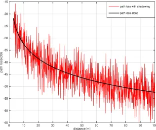
Shadowing: Shadowing is also called as slow fading or long-term fading. It is caused by the complex environment[19] and is normally distributed across an average value, which is usually
assumed to follow a Gaussian distribution. Large-scale fading is shown in Figure 2.2. The path
loss alone varies over a very long distance, usually between 100 and 1000 meters, while the
variation due to shadowing happens when the distance is between 10 and 100 meters, which is
proportional to the dimension of obstructions. As path loss and shadowing happen when the
distance is relatively large, this kind of variation is usually called large-scale fading.
Multipath: Multipath fading is also called fast fading. The transmitted signal arrives at the receiver after reflection, diffraction, and scattering results in the multipath, which is significant
in mobile communications as the mobile devices are usually at low heights and surrounded
by obstacles. This small-scale fading is referred to as Rayleigh fading since there are various
multipaths on at the receiver side with random amplitude and delay adding up to present a
Rayleigh probability density function as a total signal. The red line in Figure 2.3 shows the
2.1. RangeBasedLocalizationTechnologies 11
distance(m)
0 10 20 30 40 50 60 70 80 90 100
path loss(dB)
-65 -60 -55 -50 -45 -40 -35 -30 -25 -20 -15
path loss with shadowing
path loss alone
Figure 2.2: Path loss fading with shadowing.
distance(m)
0 10 20 30 40 50 60 70 80 90 100
path loss(dB)
-90 -80 -70 -60 -50 -40 -30 -20
path loss alone
path loss with shadowing
path loss with shadowing and multipath
Received Signal Strength Indicator technologies
Even though there are multiple options for the location-relating measurements such as ToA,
TDoA, and AoA, RSS[20] is typically preferred for indoor Wireless Local Area Network
(WLAN) localization due to its low expense and broad availability without the need for
ex-tra hardware.
Direct measurement: RSS is the simplest method of distance measurement based on the relation between the transmitted signal attenuation with distance; however, its accuracy is not
good due to the multipath fading effect of the environment. Also the positioning error is a
multiplicative factor of the range and increases proportional to the distance[21].
Received Signal Strength Indicator (RSSI) is a convenient and low-cost option for
local-ization systems as most transceiver hardware is equipped with it[22][23]. Plenty of research
has been done to investigate the relationship between the power and distance[40]. In many
experimental findings, the distance follows a power law. In free space propagation models, the
ratio between the transmitted signal power and the received signal power can be expressed as
Pr
Pt
= GtGrλ2
(4πd)2, (2.4)
where Pr is the power of the received signal, Pt is the power of the transmitted signal,Gr is
the antenna gain of the receiver,Gt is the antenna gain of the transmitter, anddis the distance
between the receiver and transmitter.
But in reality, as a result of the influence from obstacles, the path loss tends to obey a
log-normal-shadowing model as below
P(d)= P(d0)−10nlog(
d d0
)+σ, (2.5)
where P(d0) is the reference path loss at the reference distance d0 from the receiver to the
2.1. RangeBasedLocalizationTechnologies 13
is the path loss at the target point when it has a distance ofdfrom the transmitter;nis the path
loss exponent, which is usually between 2 and 5; andσis usually a Gaussian random variable
with zero mean, which reflects the attenuation due to fading.
In the embedded devices, the received signal strength is transferred to the RSS instead. The
definition is
RS S =10·log( Pr Pre f
), (2.6)
wherePre f is usually defined as 1mW andPris the received signal strength.
Fingerprinting: While the above localization technique is based on the real-time measure-ment to derive the distance, the fingerprinting technology relies on observations attempting to
match real-time measurements. As it is well known that a lot of work should be done prior
to operation as well as repeated work if the environment changes, this RSS fingerprinting
pro-vides better accuracy than direct RSS estimation[41][42]. The Microsoft Research RADAR
location system is an application for the fingerprinting based on the Wireless Fidelity (WiFi)
signal strength for indoor environments[43]. In indoor localization, GSM signal strength can
also be used to build a RSS map[44]. The RSS values for one position are recorded from all of
the nearby anchors in its communication range.
This technology usually involves a two-step process.The first step is offline or the learning
phase, the RSS measurements at different positions are recorded. During this stage, the mobile
nodes are usually held by testers and the anchor nodes record the power level of the signal
strength from the mobile nodes to set up the RSS map. The second step is an online phase
and occurs after the database has been built in the previous stage. The signal strengths are
compared to find the best match between the observed signal strength and the recorded signal
strength.
The drawback of the fingerprinting technology is its high expense, which is generally due
2.1.2
Time Based Localization
Various accurate localization systems make use of the measurements of signal travel time, as
this technology can reach centimeter-level accuracy.
Time of Arrival:The ToA technique is more complex than the RSS technique but the resulting measurement errors are less multiplicative. Time measurement using ToA is usually more
accurate than signal strength-based localization technology, as RSS is significantly affected by
obstacles and walls.
ToA calculates the distance between the reference and target nodes by computing the
trav-eling time between them. The distance between two nodes is proportional to the travel time
of the signal from one node to another[30]. Lett denotes the time when the target point is at
(x,y) astr denotes the time when the reference point position is (xr,yr). Since the speed of the
wireless signal in air is the same as the lightc, the distance dbetween them can be computed
by[26]
d= (tr−t0)c. (2.7)
However, the transmitter and receiver in ToA systems must be synchronized, which is
dif-ficult to achieve[27].
Time Difference of Arrival: The above ToA technology requires complete synchronization between the target point and the reference node, which is not possible in reality. As a result,
TDoA can be an alternative method used to lower the influence of non-synchronization.
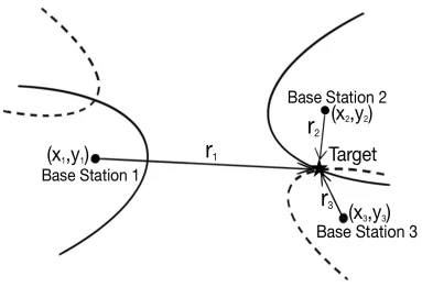
Generally, the TDoA estimation method is used to measure the time difference of the signal
from the target arriving at different base stations, as illustrated in Figure 2.4. This method
utilizes the fact that the points in the hyperbola have different constant distances to two fixed
points in the plane[25]. As a result, the target must be on the hyperbola. Usually two or
more sets of hyperbolas or at least three base stations will be needed to locate the target. As
2.1. RangeBasedLocalizationTechnologies 15
channel characteristics of the base stations are similar, the error caused by the multipath can be
reduced.
Figure 2.4: Estimated localization based on TDoA technology
TDoA achieves accurate results and is widely used in localization systems such as GPS[28]
and television[29]. However, this technique requires additional hardware to perform time
mea-surements.
2.1.3
Angle Based Localization
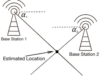
The AoA scheme is more complicated and is also affected by the multipath fading effect. AoA
technology requires at least two base stations[30] and locates the target at the intersection,
as shown in Figure 2.5. Directional antenna or antenna array are used to make the angular
measurements in AoA-based localization systems[31].
The advantage of AoA is that it does not require any synchronization between the antennas.
Also, AoA estimation can be determined with only two base stations for 2D localization or
the multipath. There are limitations, as AoA cannot reach long distances, which is a result of
large distance errors caused by angular resolution.
Figure 2.5: Estimated localization based on AoA technology
2.2
Localization Estimation Algorithms
The localization of an object in reality is estimated by requiring some physical measurements
based on its characteristics using localization technologies such as the ones discussed in the last
section. However, the localization information collected by above localization technologies is
not accurate on its own. Depending on the localization information from measurements, there
is a variety of algorithms which can be used to narrow the localization error.
2.2.1
Least square estimation
In wireless localization estimation systems, one of the most widely used methods is the Least
2.2. LocalizationEstimationAlgorithms 17
developments[33] it is clearly and concisely written in [34]. LSE is to fit a line that has the
minimal sum of squared deviation compared to a collection of existing data.
Suppose we have a user whose position is denoted by (x,y) and a base station denoted by
(xi,yi),i = 1,2, ...,N. In the first localization step, the real distance between the user and base
stationdi can be expressed as
di =
p
(x−xi)2+(y−yi)2. (2.8)
However, in range measurement, the distances usually come with an ranging error:
ˆ
di =di+ei, (2.9)
whereei demonstrates the error caused by the RSS, ToA or AoA measurements. As a result,
the Equation 2.8 should be written as
(x−xi)2+(y−yi)2= dˆi 2
. (2.10)
Expanding Equation 2.10, we get
−2xix−2yiy+x2+y2 =dˆi 2
−x2i −y2i. (2.11)
Using the linear least squares method, if we present it in matrix form, we can get
AΛ=b, (2.12)
whereA=
−2x1 −2y1 1
−2x2 −2y2 1
... ... ...
−2xN −2yN 1
,Λ= x y
x2+y2
andb=
ˆ d1 2
− x2 1−y
2 1
ˆ d2
2
− x2 2−y
2 2 ... ˆ dN 2
−x2
N −y
However, when N is large, the estimator is overdetermined and will have more than one
solution forAΛ=b. The solution of the least square problem is presented as follows: (x,y)= arg min
(x,y)
kAΛ−bk2. (2.13)
Then, the solutionAΛ≈ bcan be expressed as
ATAΛ=ATb, (2.14)
Λ=(ATA)−1ATb. (2.15)
Compared to Maximum Likelihood Estimation (MLE), which will be discussed in the
fol-lowing section, LSE is a sub-optimum localization algorithm. However, it is simpler than MLE
and provides a comparatively accurate output since it does not demand iterative calculations
and has a closed-form result.
2.2.2
Maximum likelihood estimation
MLE is a relatively simple method of estimating the parameters of a statistical model given
data. MLE can be applied to most problems and is one of the earliest techniques investigated
in the localization problems, since MLE technology is perhaps the most recognized estimation
method in statistics. It is widely recommended by Ronald Fisher[35] followed by several
developments from other authors. The aim of MLE technology is to maximize the probability of the observed data that is independent under a certain distribution. If the sample is large
enough, this statistic method will act as an effective estimator.
Assume there is a set of random samples x1, x2, ..., xn of n independent and identical
distributions f(x1|θ), f(x2|θ), ..., f(xn|θ), which are probability density functions. Here, the
given symbol indicates that the distribution is dependent on a parameterθ, which could be a
2.2. LocalizationEstimationAlgorithms 19
of independent and identically distributed random variables is
f(x1,x2, ...,xn|θ)= f(x1|θ)× f(x2|θ)×...× f(xn|θ). (2.16)
We call f(x1,x2, ...,xn|θ) the likelihood function and it is always denoted as L(θ). MLE
attempts to maximize the likelihood function L(θ) with respect to the unknown parameter θ.
L(θ) is equivalent tologL(θ) aslog is a monotonic increasing function. logL(θ) is called log likelihood function and is denoted asl(θ) as follows:
l(θ)=logL(θ)=log
n
Q
i=1
f(xi|θ)= n
P
i=1
log f(xi|θ). (2.17)
In a localization problem, the distance measurementDibetween the targetT and the anchor
Riis a random variable following Gaussian distributionN(µi, σ2) whereµiis the actual distance
between the unknown node T and the ith reference node Ri. σ2 is usually set to be a fixed
constant. Suppose the range measurements are independent from each other and let the sample
value bedi,i=1,2, ...,N.
The probability density functions ofDi are
f
i(x
)
=
√1
2π
σ
e
−(x−µi)2
2σ2
,
(2.18)
where the real distanceµi =
p
(xi−x)2+(yi−y)2. In this way, the MLE likelihood function is
presented below:
L(x,y)=
N
Q
i=1
fi(di)= N
Q
i=1
1
√
2πσe
−(di−µi)2/2σ2
=√1
2πσ N
e
−1/2σ2
N
P
i=1
(ri−µi)2
.
(2.19)
In the MLE localization process, the aim is to maximize the likelihood function L(x,y),
to solve, here we derive it as follows:
l(x,y)=logL(x,y)= Nlog(√1
2πσ)− 1 2σ2
N
P
i=1
(ri−µi)2. (2.20)
Maximizing Equation 2.20 is to minimizeu(x,y)=
N
P
i=1
(ri−µi)2/(2σ2), which is equal to figuring
out the equation set below:
∂u ∂x =
N
P
i=1
(xi−x)
µi−ri
µi = 0,
∂u ∂y =
N
P
i=1
(yi −y)µi
−ri
µi = 0.
(2.21)
By solving the localization problem using the MLE technology outlined above, the
accu-racy can be increased compared to when the multilateral range measurement information in
linear least square method is used. MLE attains the lower bound when the sample amount N
goes to infinity.
2.2.3
Cram´er-Rao Lower Bound
Cram´er-Rao Lower Bound (CRLB) provides a lower bound on the variance of the estimator
whose name is in honor of authors who derive it[36][37].
After obtaining theloglikelihood function, we also have information about other
parame-ters related to the MLE technique. The score function is the one simply present in the gradient
ofloglikelihood:
s(θ)= ∂logL(θ)
∂θ , (2.22)
where we setθ= (x,y) as the unknown parameter in the location estimation problem andL(θ)
is the likelihood function, which is also the joint density function f(X;θ), whereX : (xi,yi),i=
1,2, ...,N is the observable random variable.
2.2. LocalizationEstimationAlgorithms 21
I(θ), is defined as the matrix of the second moments of the score function[50]:
I(θ)=E[s2(θ)]=E
∂logL(θ) ∂θ
!2
. (2.23)
The Fisher information can also be expressed as
I(θ)=−E
"∂2logL(θ)
∂2θ
#
(2.24)
since
E
"∂2logL(θ)
∂2θ
#
= E "∂
∂θ
1 L(θ)
∂logL(θ) ∂θ !# = E 1 L(θ) ·
∂2L(θ)
∂θ2 −
" 1 L(θ)
∂L(θ) ∂θ
#2
=Z 1
L(θ) ·
∂2L(θ)
∂θ2 ·L(θ)dθ−E
∂logL(θ) ∂θ
!2 (2.25)
and the first moment of the score which is the expectation of the score is 0:
Z 1 L(θ) ·
∂2L(θ)
∂θ2 ·L(θ)dθ=
Z ∂2L(θ)
∂θ2 dθ
= ∂θ∂22 Z L(θ)dθ
= ∂θ∂22 ·1= 0,
(2.26)
Thus, the Fisher information is also called the variance of the score.
Now, we know that X is a vector of random variables (xi,yi),i = 1,2, ...,N and the joint
density function is f(X;θ) whereθis the target location (x,y) in the localization problem. The
any unbiased estimator ofθ. The Cram´er-Rao inequality is
Var[θ(X)]≥ 1
I(θ), (2.27)
whereI(θ)−1is the CRLB. This inequality tells us that in the localization problem the precision
to which we can estimate the targetθ: (x,y) is basically limited by the Fisher information.
2.3
Sensor Measurements
Smartphones not only provide provide RADAR and GPS but also offer a variety of Inertial
Navigation System (INS) sensors, such as accelerometer, magnetometer, gyroscope, whose
in-formation can be used to locate the portable devices. These sensors present useful inin-formation
to locate and track users.
2.3.1
Accelerometer
In instances of acceleration of the device, the accelerometer can not only be used to locate a
tar-get, but also can be analyzed to detect the activities of the user. Almost all recent smartphones
have three-axial accelerometers, making them a good choice for pedestrian dead reckoning
and locating users. Accelerometers can help detect human activities such as going upstairs
or downstairs and walking which is ideal for patients detection in medical field. In addition,
accelerometer values can be used for calculating the velocity and location of a robot[39].
However, the accelerometer itself has measurement error. The direct evidence is that while
placing a smartphone on a desk or keeping it static in hand, the sensor will report the
smart-phone is moving. Although the readings from accelerometer along three axes are small, it can
accumulate to a large error with time. Efforts have been done due to this weakness. One of
2.4. ChapterSummary 23
2.3.2
Magnetometer
Magnetometer measures the earth’s magnetic field strength. Magnetic field sensors’ directions
are determined with respect to the North Magnetic Pole on the surface of the Earth and the unit used is microtesla (µT). Compass is one of the application based on this feature which can
give orientation of the user. However, this sensor is very sensitive to the surroundings such as
electronic devices or buildings materials, which can be regarded as noise. It has been revealed
in [38] that disturbances of the magnetic field can be utilized to locate the users.
2.3.3
Gyroscope
Gyroscopes are used to assist the magnetometer as well as the accelerometer to increase the
precision of localization. Radians per second (rad/s) are measured using the gyroscope sensor,
which shows the difference of the smartphones’ rotation, namely, the angular velocity. Even
though the magnetic field sensor is slower than the gyroscope, the gyroscope can only be
utilized to assist with the magnetometer for higher precision since, unlike the magnetometer,
the gyroscope cannot determine the orientation of the phone. Thus, a combination of these
motion sensors can provide an overall good performance since the magnetic field sensor offers
long-term information while the gyroscope provides quick adjustments to the short-term data.
2.4
Chapter Summary
In this chapter, we review the techniques and algorithms used in localization system.
Po-sitioning techniques are classified into two categories, range-based and range-free schemes.
Range-based localization technologies, including signal-based, time-based and angle-based
technologies, are discussed first. LSE and MLE are both regression estimation methods used
to minimize the error of localization and maximize the probability of measurements
respec-tively; they are also analyzed in details. Estimator based on CRLB is another algorithm that
end to give a general view on INS sensors which can provide additional assistance to
Chapter 3
Optimum Reference Node Deployment for
Indoor Localization Based on the Average
Mean Square Error Minimization
Considering all the localization systems, a critical common issue needs to be tackled is to
deter-mine the physical positions of reference nodes. In [24], it shows that the placement of reference
nodes has substantial impact on the positioning accuracy. Therefore, finding the optimum
lo-cations for reference nodes are vital in nearly every localization systems and reference nodes
placement strongly affects the quality of localization. In this chapter, average mean square
error is minimized to obtain best average localization performance over certain regions.
3.1
Introduction
Many localization methods proposed have been proposed recently to find the optimum
refer-ence nodes to reduce the localization estimation error. In [45], referrefer-ence anchors are optimized
to improve the performance of linear least squares and weighted least squares algorithm in
RSS-based localization.
Using the GPS for indoor localization is challenging as the GPS signal is significantly
at-tenuated or completely blocked by the building. In achieving indoor localization, a set of
trans-mitters from wireless communication networks are often used as reference nodes to localize
target nodes with unknown locations. The accuracy of such localization process is
consider-ably affected by the spatial distribution of the reference nodes with respect to the target node
to be localized. Hence, deploying the reference nodes at best locations will notably increase
the localization precision. In this chapter, a novel reference nodes deployment scheme is
in-troduced which minimizes the average Mean Square Error (MSE) of the localization over the
area of interest with certain shape. The proposed scheme is evaluated for deploying the
refer-ence nodes in the circular, square, and hexagonal localization regions. The proposed scheme is
validated and illustrated by numerical simulations.
In wireless networks, CRLB is usually defined as a benchmark so that we can know how
good an estimator will possibly do[13]. It also helps us compare the performances between
dif-ferent localization estimations[46]. Average CRB is derived in [21] based on RSS localization
to study the nonlinear least square solution presented. Another ToA-based average CRLB in
NLoS environment can be found in [47]. According to [47] and [48], CRLB provides a lower
bound on the MSE of a position estimate. In some cases, average MSE is used to evaluate
practical estimators’ performance in positioning systems. A reference node selection strategy
is proposed in [49] which minimizes the average MSE in the TDoA based position system. In
this paper, we are interested in the first two diagonal terms of the CRLB which provide the
Minimum Mean Square Error (MMSE) of the position estimation. We propose a reference
nodes deployment scheme which determines the optimum locations by minimizing MMSE
over selected areas which can be circle, hexagon or square. Besides, our scheme can also be
3.2. MinimumMeanSquareErrorScheme 27
3.2
Minimum Mean Square Error Scheme
As mentioned above, ToA is based on the signal propagation time measurement between nodes.
If (xT,yT) is the location of a target node T being localized and (xi,yi) is the location of thei-th
reference node localizing T,
di(x,y)=
p
(xT−xi)2+(yT−yi)2 (3.1)
is the distance between T and thei-th reference node. In this case, the signal propagation time
is measured as
ti =
di
c +ζi, i=1, ...,N, (3.2)
where constant c is the signal propagation speed, and ζi is the measurement noise which is
usually modeled as a zero-mean Gaussian random variable with a constant variance σ2i[13],
andNis the number of reference nodes. In this case, the location of T is obtained based on the
measured time values (t1,t2, . . . ,tN). In addition, if ( ˆxT,yˆT) is the estimated location of T, then
the localization error is obtained as
e= p( ˆxT−xT)2+(ˆyT −yT)2, (3.3)
which can be used to compare the accuracy between different localization estimators.
In addition to the accurate estimation of the distances between the target node and any of
the reference nodes, the topology of the reference nodes with respect to the target node can also
significantly affect the performance of the target node localization. Hence, in order to get the
best estimation of the target node, it is more efficient to use the reference nodes with optimum
locations for locating the target node.
The average mean square error of ederived in (3.3) is a good figure of merit to select the
in [47] and [48] that the MMSE of the ToA localization scheme is given by
M MS ET oA=
c2ΣNL
i=1σ −2 i
ΣNL
i=1Σ i−1
j=1σ −2
i σ
−2
j sin
2(θ i−θj)
, (3.4)
wherecis the speed of the light,σi andσj represent theith and jth ToA measurement errors
respectively, NL is the number of reference nodes. θi = tan−1( y−yi
x−xi) and it denotes the angle
between the ith reference node and the target node. (x,y) and (xi,yi) are the positions of the
target node and theith reference node, respectively.
In order to get the average MMSE within a certain range, we have to get the average MMSE
expression. The ToA-based average MMSE result can be expressed as
M MS E(x,y)= c
2σ2N
PN−1
i=1
PN
j=i+1(sinθi j)2
, (3.5)
whereθi j = θi−θj and N is the number of reference nodes. σ2denotes the ToA measurement
error.
In the usual situation where has 3 reference nodes , we can simplify the average MMSE
expression from (3.5) to
M MS E(r, θ)= 3c
2σ2
sin2θ12+sin2θ23+sin2θ13
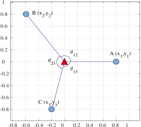
, (3.6)
where θ12, θ23 and θ13 denote the angular distances between every two reference nodes as
shown in Figure 3.1. The target node is in the center of the figure presented as triangle and the
3 reference nodes are randomly distributed which are circles in Figure 3.1. In this paper, we set
cσequal to 1. Also, sin2θ12, sin2θ23, sin2θ13can be derived by the vector product expression
a×b=kak · kbksinθ, (3.7)
3.3. AverageSchemeInCertainLocalizationRegions 29
-0.8 -0.6 -0.4 -0.2 0 0.2 0.4 0.6 0.8 1
-0.8 -0.6 -0.4 -0.2 0 0.2 0.4 0.6 0.8 1 A (x 1,y1) B (x
2,y2)
C (x 3,y3)
θ 12 θ 23 θ 13
Figure 3.1: Illustration of 3 Reference Nodes in the Mean Square Error Minimization Problem
3.3
Average Scheme In Certain Localization Regions
We consider a three-reference-node localization scenario to localize a target node T located in
a determined localization region. We analyze three different cases separately. In the first case,
one reference node is assumed to be fixed at the center of the localization region, which with
refer to it as the base station, whereas the other two nodes are deployed to help the base station
to localize T which minimize the localization error over this region.
At first, we assume the nodes are in an unit circle. In this circular region, there are one
ref-erence node O with known location in the center and two refref-erence nodes A, B with unknown
location within the circle, then the parameters in average MMSE expression from (3.6) can be
calculated out as
sin2θ12=
r2 Asin
2θ
r2
A+r2−2rrAcosθ
, (3.8)
sin2θ23=
(rrBsin(θ−θ0)−rrAsinθ+rArBsinθ0)2
(r2+r2
B−2rrBcos(θ−θ0))(r 2
A+r2−2rrAcosθ)
and
sin2θ13 =
r2 Bsin
2(θ−θ 0)
r2+r2
B−2rrBcos(θ−θ0)
. (3.10)
Here,rAandrBare the distances between O and A, B respectively.ris the distance between
T and O.θis the angular distance between the segments which connect A, T with O.θ0denotes
the angular distance between the segments which connect A, B with O.
The average MMSE result within this unit circle is considered as
M MS E = 1 π
Z 2π
0
Z 1
0
M MS E(r, θ|rA,rB, θ0)rdrdθ. (3.11)
In this way, the optimum locations of reference nodes A, B can be obtained by minimizing
the average MMSE expression.
(ˆrA,rˆB,θˆ0)= argminM MS E (3.12)
In this case, we also consider the square region as well as the hexagonal region to prove the
flexibility of our scheme. For these two regions, the parameters of average MMSE expression
in (3.6) are (3.13), (3.14) and (3.15).
sin2θ12=
(xAyC− xCyA)2
(x2C+y2C)(x2A+ x2C−2xAxC+y2C+y2A−2yAyC)
, (3.13)
sin2θ23 =
(xByC+ xAyB+xCyA−xByA−xAyC− xCyB)2
(x2B+ x2C−2xBxC+y2C+y2B−2yByC)(x2A+x2C−2xAxC+y2C+y2A−2yAyC)
, (3.14)
sin2θ13 =
(xByC− xCyB)2
(x2 C+y
2 C)(x
2 B+x
2
C−2xBxC+y 2 B+y
2
C−2yByC)
. (3.15)
The average MMSE expression within a square whose side is 1 is as follow:
M MS E = Z 12
−12
Z 12
−12
3.3. AverageSchemeInCertainLocalizationRegions 31
Similarly, the average MMSE expression within a hexagon whose side is 1 is as follow:
MMSE=2 √ 3 9 Z √ 3 2 − √ 3 2 Z 1 −1
MMSE(xC,yC|xA,yA,xB,yB)dxdy
−4 Z 0 − √ 3 2 Z − √ 3 3 x−1
−
√ 3 2
M MS E(xC,yC|xA,yA,xB,yB)dxdy.
(3.20)
By minimizing the average MMSE result, we can get the positions of optimum reference
nodes by
( ˆxA,yˆA,xˆB,yˆB)=argminM MS E (3.21)
in square region or in hexagonal region.
In the second case, we consider a situation where there are two reference nodes A and B
with known location at central axis of a region. In circular region, we set A to (1,0) or (13,0)
and B to (-1,0) or (-13,0) respectively. C is the reference node with unknown location within the
region that we want to obtain. In this assumption, the parameters in (3.6) are
sin2θ12 =
(rrBsinθ−rrAsinθ)2
(rA2 +r2−2rr
Acosθ)(rB2 +r2−2rrBcosθ)
, (3.22)
sin2θ23 =
(rArCsinθ0−rrAsinθ+rrCsin(θ−θ0))2
(r2+r2
C−2rrCcos(θ−θ0))(r 2
A+r2−2rrAcosθ)
, (3.23)
and
sin2θ13=
(rBrCsinθ0−rrBsinθ+rrCsin(θ−θ0))2
(r2B+r2−2rr
Bcosθ)(r2+r2C−2rrCcos(θ−θ0))
. (3.24)
Similarly, in square and hexagonal region, the parameters in (3.6) are
sin2θ12 =
(xByC−xBy−xyC+xCy)2
[(xB−x)2+y2][(xC−x)2+(yC−y)2]
, (3.25)
sin2θ23 =
(xAyC−xAy−xyC+xCy)2
[(xA−x)2+y2][(xC−x)2+(yC−y)2]
and
sin2θ13=
(xAy−xBy)2
(x2
B+x2−2xxB+y2)(x 2
A+x2−2xxA+y2)
. (3.27)
But in hexagonal region, A and B are set to be (
√ 3
6 ,0) and (-√
3
6 ,0) or ( √
3
2 ,0) and (-√
3 2 ,0).
Actually in reality, there is no reference node with known location in advance for many cases. So at last, we consider the third case where we want to obtain three reference nodes
A, B and C without prior location information. We present the parameters in (3.6) as (3.28),
(3.29) and (3.30) in circular region where θA, θB, θC, θT denote the angle between the x-axis
through the center of the circle and segment which connects A, B, C, T with the center of the
circle, respectively.
sin2θ12=
((rBcosθB−rTcosθT)(rCsinθC−rTsinθT)−(rBsinθB−rTsinθT)(rCcosθC−rTcosθT))2
(r2 B+r
2
T−2rBrTcos(θB−θT))(r 2 C+r
2
T−2rCrTcos(θC−θT))
(3.28)
sin2θ23 =
((rBcosθB−rTcosθT)(−rTsinθT)−(rBsinθB−rTsinθT)(rA−rTcosθT))2
(r2 B+r
2
T−2rBrTcos(θB−θT))(r 2 A+r
2
T−2rArTcos(θA−θT))
(3.29)
sin2θ13=
((rAcosθA−rTcosθT)(rCsinθC−rTsinθT)−(rAsinθA−rTsinθT)(rCcosθC−rTcosθT))2
(r2A+rT2−2rArTcos(θA−θT))(rC2 +rT2−2rCrTcos(θC−θT))
(3.30)
In square and hexagonal region, the parameters in (3.6) are
sin2θ12=
[(xB−xT)(yC−yT)−(yB−yT)(xC−xT)]2
[(xB−xT)2+(yB−yT)2][(xC−xT)2+(yC−yT)2]
, (3.31)
sin2θ23=
[(xB−xT)(yA−yT)−(yB−yT)(xA− xT)]2
[(xB−xT)2+(yB−yT)2][(xA− xT)2+(yA−yT)2]
(3.32)
and
sin2θ13=
[(xA−xT)(yC−yT)−(yA−yT)(xC−xT)]2
[(xA−xT)2+(yA−yT)2][(xC− xT)2+(yC−yT)2]
. (3.33)
3.4. SimulationResults 33
the optimum position information can be obtained by minimizing
( ˆxA,yˆA,xˆB,yˆB,xˆC,yˆC)=argminM MS E. (3.34)
All the implements above will be simulated at one time and we will get the results at the
same time.
Until now, we provide three common designs in three different shapes of region. This not
only proves that our scheme is flexible but also gives a guidance for starting to set a localization
system and obtain the optimum reference nodes placement.
3.4
Simulation Results
In this section, we present the numerical optimization results for the three reference nodes po-sitioning in different scenarios, based on the deployment region of the target node as following.
3.4.1
Circular Region
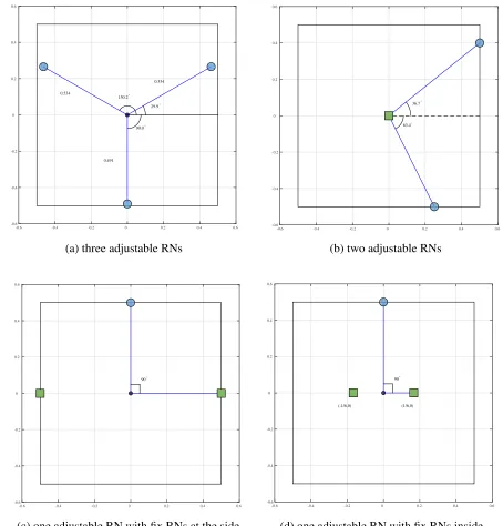
In Figure 3.2, the optimum deployment topologies are shown when the location of the reference
nodes are unknown (Figure 3.2-(a)), one reference node is fixed at the center of the region
(Figure 3.2-(b)), two reference nodes are fixed in the region (Figure 3.2-(c) and -(d)).
As shown in Figure 3.2-(a), assuming three reference nodes can be deployed anywhere in
the circular region, the best structure is when the reference nodes have equiangular distances,
i.e., equal to 120◦, around the center of the region. Also, their distances to the center are equal,
which is 0.901 times the radius of the region. Figure 3.2-(b) shows the optimum case when a
reference node, i.e., one base station, is located at the center of the circular region and two other
-1 -0.8 -0.6 -0.4 -0.2 0 0.2 0.4 0.6 0.8 1 -1 -0.8 -0.6 -0.4 -0.2 0 0.2 0.4 0.6 0.8 1 120° 120° 120° 0.901 0.901 0.901
(a) three adjustable RNs
-1 -0.8 -0.6 -0.4 -0.2 0 0.2 0.4 0.6 0.8 1
-1 -0.8 -0.6 -0.4 -0.2 0 0.2 0.4 0.6 0.8 1 99.0°
(b) two adjustable RNs
-1 -0.8 -0.6 -0.4 -0.2 0 0.2 0.4 0.6 0.8 1
-1 -0.8 -0.6 -0.4 -0.2 0 0.2 0.4 0.6 0.8 1 90°
(c) one adjustable RN with fix RNs at the side
-1 -0.8 -0.6 -0.4 -0.2 0 0.2 0.4 0.6 0.8 1
-1 -0.8 -0.6 -0.4 -0.2 0 0.2 0.4 0.6 0.8 1 (1/3,0) (-1/3,0) 90°
(d) one adjustable RN with fix RNs inside
3.4. SimulationResults 35
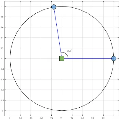
localization. As the figure depicts, the optimum positions for the two reference nodes are on the circumference of the circle with angular distance 99.0◦
with respect to the center of the region.
Figure 3.2-(c) and -(d) show the cases where two base stations are located on the diameter
of the region symmetrically on two sides of the center, within and on the circumference of
the circle, respectively. As seen, in both cases, the best position of the third reference node
cooperating with the two base stations is on the intersection of the circumference of the circle
and the perpendicular bisector of the base stations crossing line.
3.4.2
Hexagonal Region
Similar to the circular region case, the reference nodes placements shown in Figure 3.3 present
three optimum localization conditions when no reference node is fixed (Figure 3.3-(a)), one
reference node is fixed (Figure 3.3-(b)), and two reference nodes are fixed (Figure 3.3-(c) and
-(d)).
For the first case where no reference node is fixed, the optimum locations of the three
ref-erence nodes are shown in Figure 3.3-(a). In this case, the refref-erence nodes form an equilateral
triangle within the hexagon which means they have equal angular distances 120◦ around the
center of the region. In addition, the distances between the reference nodes and the center point
are 0.804 times the side of the hexagonal region. In Figure 3.3-(b), a reference node as a base
station is fixed at the center of hexagonal region and the other two reference nodes assist the
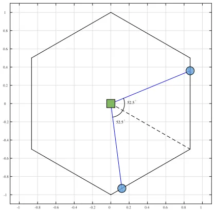
base station to locate the target node in this region. From the result, we can find that the best
positioning for the two reference nodes are at the boundary of the region with angular distance 105.0◦
with respect to the center point. In Figure 3.3-(c) and -(d), two base stations are locate
on the central axis of the hexagonal region, symmetrically on two sides of the center point
and separated one third of the diameter. The figures show that they have the same optimum
-1 -0.8 -0.6 -0.4 -0.2 0 0.2 0.4 0.6 0.8 1 -1 -0.8 -0.6 -0.4 -0.2 0 0.2 0.4 0.6 0.8 1 0.804 0.804 0.804 60.0° 60.1° 180.0°
(a) three adjustable RNs
-1 -0.8 -0.6 -0.4 -0.2 0 0.2 0.4 0.6 0.8 1
-1 -0.8 -0.6 -0.4 -0.2 0 0.2 0.4 0.6 0.8 1 52.5° 52.5°
(b) two adjustable RNs
-1 -0.8 -0.6 -0.4 -0.2 0 0.2 0.4 0.6 0.8 1
-1 -0.8 -0.6 -0.4 -0.2 0 0.2 0.4 0.6 0.8 1 90°
(c) one adjustable RN with fix RNs at the side
-1 -0.8 -0.6 -0.4 -0.2 0 0.2 0.4 0.6 0.8 1
-1 -0.8 -0.6 -0.4 -0.2 0 0.2 0.4 0.6 0.8 1 (0.289,0) (-0.289,0) 90°
(d) one adjustable RN with fix RNs inside
3.4. SimulationResults 37
the base stations.
3.4.3
Square Region
In Figure 3.4, the optimum deployment topologies are shown for the square region, when the
location of the three reference nodes are unknown (Figure 3.4-(a)), one reference node is fixed
at the center of the region (Figure 3.4-(b)), and two reference nodes are fixed in the region
(Figure 3.4-(c) and -(d)).
As depicted by Figure 3.4-(a), the optimum case when the the reference nodes can be located anywhere on the square region is similar to circular and hexagonal region cases, i.e.,
the angular separation between any two reference nodes is close to 120◦ and they maximally
spread on the region. In addition, for the case where one reference node is fixed in the center
of the region as a base station, the optimum location of the other two reference nodes are
on the boundary of the square region with angular separation around 100◦, which is close to
what have been obtained for the circular and hexagonal regions. Furthermore, for the two base
station case where two reference nodes are fixed in the region or on the boundary, as shown
by Figure 3.4-(a) and Figure 3.4-(b), respectively, the optimum location of the third reference
node is similar to those of the circular and hexagonal regions, i.e., on the boundary and on the
perpendicular bisector of the base stations crossing line.
In fact, our proposed scheme can be used in any shape of region and the number of the base
stations or the reference nodes with no prior localization can also be different. Besides, when
our scheme is applied to the situation where there are 3 unknown base stations, it can in fact be
used to establish a localization system in any wireless network.
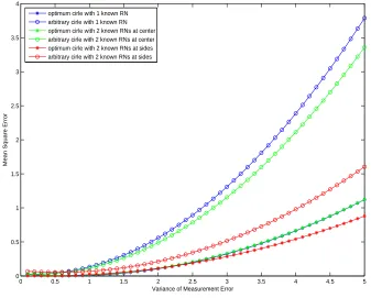
Figure 3.5 shows the 50-iteration simulation results which compare the situations when we
-0.6 -0.4 -0.2 0 0.2 0.4 0.6 -0.6 -0.4 -0.2 0 0.2 0.4 0.6 0.534 0.534 0.491 29.9° 150.2° 90.0°
(a) three adjustable RNs
-0.6 -0.4 -0.2 0 0.2 0.4 0.6
-0.6 -0.4 -0.2 0 0.2 0.4 0.6 36.7° 63.4°
(b) two adjustable RNs
-0.6 -0.4 -0.2 0 0.2 0.4 0.6
-0.6 -0.4 -0.2 0 0.2 0.4 0.6 90°
(c) one adjustable RN with fix RNs at the side
-0.6 -0.4 -0.2 0 0.2 0.4 0.6
-0.6 -0.4 -0.2 0 0.2 0.4 0.6 (1/6,0) (-1/6,0) 90°
(d) one adjustable RN with fix RNs inside
3.5. ChapterSummary 39
nodes randomly selected where we change location of one reference node among the optimum
locations. In the simulation, we select four nodes which are in the center from four different
quadrants as the target nodes and the distance between them and the central point is 0.5 in
circular scenario. With iterations increasing, the variance of noise is increasing as well. As
we can see in Figure 3.5, the accuracy can be increased by using our proposed reference nodes
selection scheme.
0 0.5 1 1.5 2 2.5 3 3.5 4 4.5 5
0 0.5 1 1.5 2 2.5 3 3.5 4
Variance of Measurement Error
Mean Square Error
optimum cirle with 1 known RN arbitrary cirle with 1 known RN optimum cirle with 2 known RNs at center arbitrary cirle with 2 known RNs at center optimum cirle with 2 known RNs at sides arbitrary cirle with 2 known RNs at sides
Figure 3.5: Mean Square Error Comparison Between Optimum RNs and Arbitrary RNs in Circular Region
3.5
Chapter Summary
In this chapter, we propose a general scheme in determining the optimum reference nodes
de-ployment scheme. For illustration and demonstration for the flexibility of the scheme, we
sim-ulate our scheme in circular, hexagonal and square positioning regions. The proposed method
be practical when extending an existed localization system. As the average positioning
per-formance was carried out, the best locationing perper-formance of the reference node deployment
could be determined as the lowest MSE average value within a certain area. It is shown from