Simulation of Heterogeneous Colloidal Particles Immersed in Liquid Crystals

(1)

Scholarship@Western

Electronic Thesis and Dissertation Repository

4-22-2016 12:00 AM

Simulation of Heterogeneous Colloidal Particles Immersed in

Liquid Crystals

Setarehalsadat Changizrezaei The University of Western Ontario

Supervisor

Prof. Colin Denniston

The University of Western Ontario Graduate Program in Physics

A thesis submitted in partial fulfillment of the requirements for the degree in Master of Science © Setarehalsadat Changizrezaei 2016

Follow this and additional works at: https://ir.lib.uwo.ca/etd

Part of the Condensed Matter Physics Commons, and the Statistical, Nonlinear, and Soft Matter Physics Commons

Recommended Citation Recommended Citation

Changizrezaei, Setarehalsadat, "Simulation of Heterogeneous Colloidal Particles Immersed in Liquid Crystals" (2016). Electronic Thesis and Dissertation Repository. 3670.

https://ir.lib.uwo.ca/etd/3670

This Dissertation/Thesis is brought to you for free and open access by Scholarship@Western. It has been accepted for inclusion in Electronic Thesis and Dissertation Repository by an authorized administrator of

(2)

Abstract

This thesis describes an investigation of interactions between colloidal particles immersed in a liquid crystal. The presence of colloidal particles in the liquid crystal distorts the director field distorted from its uniform orientation. These elastic distortions produce topological defects around the particles, which induce anisotropic interactions between them, and these anisotropic interactions can be used to manufacture non-closed packed colloidal crystals, such as diamond lattices, which are interesting in photonic applications. First, different types of liquid crys-tals, the mathematical tools to describe the anisotropic nature of liquid cryscrys-tals, the Landau-de Gennes free-energy model to investigate the particle’s interaction, and different kinds of topo-logical defects are described. Moreover, previous work regarding the interaction of particles with the same applied boundary conditions in both nematic and cholesteric liquid crystal are discussed. Second, the lattice Boltzmann method is introduced in order to couple the molecu-lar dynamics particles to the computational fluid mesh, and the simulation is performed in the open source molecular dynamics package, LAMMPS. Next, we explore anisotropic interac-tions with minima at specific orientainterac-tions of particles with heterogeneous boundary condiinterac-tions inside both nematic and cholesteric liquid crystals, which have not been observed so far. The results show that when particles are put at different distances and angles with respect to each other, new types of defect structures are produced, depending on the relative distances and di-rections. In the cholesteric liquid crystal, the value of pitch affects the defect structures and induced forces.

Keywords: Liquid Crystal, Lattice Boltzmann

(3)

The work presented in this thesis was done in collaboration with my supervisor, Prof. Colin Denniston. Chapter 3 will form the basis for a publication that will be co-authored with my supervisor.

(4)

Acknowlegements

First and foremost, I am deeply grateful to my supervisor, Professor Colin Denniston, for his guidance and support throughout my graduate studies at the University of Western Ontario. It was a great honor for me to work with such creative, brilliant, and knowledgeable supervisor. I also would like to extend my gratitude and affection to my beloved parents, Fatemeh and Mohsen, and my two brothers Saeed and Hamid, who supported me throughout my academic life.To them, I owe all I have ever accomplished.

(5)

Abstract i

Co-Authorship Statement ii

Acknowlegements iii

List of Figures vi

List of Tables viii

List of Appendices ix

List of Abbreviations x

1 Introduction 1

1.1 Liquid Crystal Classes . . . 2

1.2 Liquid Crystal Phases . . . 2

1.2.1 Nematic . . . 2

1.2.2 Cholesteric . . . 4

1.3 Order Parameter . . . 5

1.4 Landau-de Gennes Theory of Liquid Crystals . . . 6

1.5 Liquid Crystal Hydrodynamics . . . 10

1.6 Topological Defects . . . 11

1.7 Colloidal Particles . . . 13

2 Methodology 19 2.1 Introduction . . . 19

2.2 Lattice Boltzmann Method: Historical Background . . . 20

2.3 The Boltzmann Equation . . . 21

2.4 Lattice Boltzmann Method . . . 23

2.5 Modeling a Liquid Crystal Through LBM Algorithm . . . 27

2.6 Coupled LB-MD Method . . . 29

2.6.1 Particle-Fluid Interaction . . . 29

2.7 Summary . . . 32

3 Results 33 3.1 Individual Spheres in Nematic . . . 35

(6)

3.1.1 Interaction of Two Particles Immersed in a Nematic Liquid Crystal . . 36 3.2 Interaction of Particles Immersed in a Cholesteric Liquid Crystal . . . 38 3.3 Discussion . . . 65

4 Conclusions 67

Bibliography 71

A Copyright Permissions 77

Curriculum Vitae 79

(7)

1.1 Different states of matter . . . 2

1.2 Chemical structure of 4pentyl-4-cyanobiphenyl (5CB). . . 3

1.3 Shear flow. . . 4

1.4 Cholesteric Liquid Crystal . . . 4

1.5 The distribution of molecular axes around the average alignment direction n . . 5

1.6 The Landau free energy of a nematic liquid crystal as a function of the scalar order parameter S. . . 7

1.7 Elastic distortions in liquid crystal . . . 8

1.8 Different Surface Boundary Conditions . . . 9

1.9 Topological defects of different strengths . . . 12

1.10 Hyperbolic Hedgehog. . . 13

1.11 Possible defects around the colloidal particles depending on molecule anchor-ing on their surfaces. In a) the sphere has planar anchoranchor-ing and in b) the sphere has perpendicular anchoring. The pink lines correspond to contour plot of posi-tions around the collidal particles where the scalar order parameter drops 15% of the bulk value. In both a) and b) the director is shown at the surface of spheres. . . 14

1.12 Boojums on the surface of the colloidal particles when they get close each other along the director in nematic. [1] . . . 15

1.13 Defect structures around the colloidal particles in cholesteric liquid crystal . . . 16

1.14 Defect-bonded chain [2] . . . 17

1.15 a) Free energy as a function of their particle-particle separation b) Angular separation of defect points [2] . . . 17

1.16 Free energy as a function of the angular positioning of the particles relative to the twist axis [2] . . . 18

2.1 Different lattice configuartions . . . 25

2.2 Spherical objects with different number of nodes . . . 29

2.3 P1 is affected by node i by the ratio 0f ₍_∆A_X1₎2 . . . 30

3.1 Schematic of our system where the periodic boundary conditions are imposed in the x and y directions, the fixed walls are located in the z direction, and the liquid crystal molecules are set to be parallel on the walls. . . 34

(8)

3.2 The defects and their images for isolated particles in a nematic liquid crystal. In (a) and (c) the sphere has planar anchoring and in (b) and (d) the sphere has perpendicular anchoring. The director is shown on the surface of the sphere in (a) and (b) and the sphere is not shown in (c) and (d), so that the image defects are visible. . . 36 3.3 Defect structures of particles at distance of 0.125µm . . . 39 3.4 Plot of interaction energy for the particles immersed in the nematic liquid

crys-tal in a) 2D and b)3D. . . 40 3.5 Plot of director field around the particles inside nematic with separation of

0.125µm . . . 41 3.6 Defect structures of particles at distance of 0.125µm in the cholesteric LC(pitch=1.5µm) 43 3.7 Defect structures of particles at distance of 0.25µm in the cholesteric LC(pitch=1.5µm)

44

3.8 Defect structures of particles at distance of 0.375µm in the cholesteric LC(pitch=1.5µm) 45 3.9 Defect structures of particles at distance of 0.375µm in the cholesteric LC(pitch=1.5µm)

with different perspective . . . 46 3.10 Defect structures of particles at distance of 0.5µm in the cholesteric LC(pitch=1.5µm) 47 3.11 Plot of interaction energy for the particles immersed in the cholesteric liquid

crystal with pitch value of 1.5µm in a) 2D and b)3D. . . 48 3.12 Defect structures of particles at distance of 0.125µm in the cholesteric LC(pitch=3µm) 52 3.13 Plot of interaction energy for the particles immersed in the cholesteric liquid

crystal with pitch value of 3µm in a) 2D and b)3D. . . 53

3.14 Defect structures of particles at distance of 0.125µm in the cholesteric LC(pitch=1.125µm) 54 3.15 Different perspective of defect structures of particles at distance of 0.125µm in

the cholesteric LC(pitch=1.125µm) . . . 55

3.16 Defect structures of particles at distance of 0.1875µm in the cholesteric LC(pitch=1.125µm) 56 3.17 Different perspective of defect structures of particles at distance of 0.1875µm

in the cholesteric LC(pitch=1.125µm) . . . 57

3.18 Defect structures of particles at distance of 0.25µm in the cholesteric LC(pitch=1.125µm) 58 3.19 Different perspective of defect structures of particles at distance of 0.25µm in

the cholesteric LC(pitch=1.125µm) . . . 59 3.20 Plot of interaction energy for the particles immersed in the cholesteric liquid

crystal with pitch value of 1.125µm in a) 2D and b)3D. . . 60 3.21 Generated defects around the particles in nematic liquid crystal onto XZ plane

while separated 0.125µm from each other . . . 61 3.22 2D contour plot of interaction energy of 2 particles in nematic LC . . . 62 3.23 Plot of director field for different particle-particle separations when θ=0◦and

the particles are confined in XZ plane. . . 63 3.24 Generated defects around the particles in nematic liquid crystal onto XZ plane

while separated 0.125µm from each other . . . 64 3.25 2D contour plot of interaction energy of 2 particles in the cholesteric LC(pitch=1.125µm) 65

(9)

3.1 Parameters . . . 35

(10)

List of Appendices

Appendix A Copyright Permissions . . . 77

(11)

LBM Lattice Boltzmann Method

MD Molecular Dynamics

LAMMPS Large-Scale Atomic/Molecular Massively Parallel Simulator

(12)

Chapter 1 Introduction

Solid, liquid and gas are three distinct phases which most of people learn about in elementary school. There are more than these three phases, and one important for this thesis is called a liquid crystal. A new and promising research area in physics and chemistry was established by the discovery of an Austrian botanist, Friedrich Reintizer [3]. In the process of melting a certain compound, he realized that the solid had a transition toward a muddy liquid at about 145.5◦C, and as he increased the temperature, it transformed to a clear liquid at about 178.5◦C. This implied a new state of matter existed, which he called a liquid crystal, which is shown in figure 1.1. Liquid crystal is considered as a mesophase, meaning an intermediate phase exist-ing between solid and liquid [4].

Colloidal crystals are composed of an array of micro- or nano-particles, which can be rep-resented as a medium with a periodic structure of dielectric constant. Therefore, they can be used as photonic crystals. One of the ideal methods to fabricate such crystals is self-assembly of colloidal particles[5]. In an isotropic (simple) fluid, the colloidal particles create close-packed crystals such as fcc and hcp, which do not show a “complete band gap”, meaning light with specific frequencies cannot be propagated through the crystal. However, the particles must experience a non-isotropic interaction to form non-close-packed structures such as a diamond lattice, which show a complete band gap. As a result, we are motivated to investigate colloids

(13)

(a) Solid (b) Nematic liquid crystal (c) Liquid

Figure 1.1: Different states of matter

in a liquid crystal due to its anisotropic nature. This kind of nature generates distortions which induce forces between the particles that do not exist in an isotropic fluid [6].

1.1 Liquid Crystal Classes

Liquid crystals have been classified into two different groups: thermotropic and lyotropic. In a thermotropic liquid crystal, temperature is the most important factor. It controls the liquid crystal behavior, which is mainly focused on in our work. On the other hand, when am-phiphilic molecules are added into a solvent like water, a lyotropic liquid crystal is formed. Each molecule has a hydrophobic tail and a hydrophilic head. So when they are mixed into water, the hydrophilic heads attracts water, but the hydrophobic tails avoids water [3]. If the concentration is high enough, a liquid crystal state is achieved.

1.2 Liquid Crystal Phases

1.2.1 Nematic

(14)

1.2. LiquidCrystalPhases 3

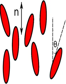
molecules show long range orientational order, however there is no translational order [7].This kind of behavior dictates anisotropic properties, which cannot be observed in simple fluids. Most molecules that form a nematic look like a rod. One of the common rod-like liquid crystal compounds is 4-Pentyl-4’-cyanobiphenyl (5CB). Its chemical structure is shown in figure 1.2. In our work, the material we have chosen to model has the similar properties of 5CB.

Figure 1.2: Chemical structure of 4pentyl-4-cyanobiphenyl (5CB).

In a nematic, the directions -ˆn and ˆn are equivalent. The properties of liquid crystals have different responses in different directions, as demonstrated by Miesowicz viscosity co-efficients [8].

In 1935, Meisowicz decided to find the viscosity of a nematic liquid crystal. As is shown in figure 1.3, the nematic liquid crystal is confined by two parallel walls in y-z plane and a shear flow is applied in a way that the velocity is in the z direction and the velocity gradient is in the x direction. He performed his experiment for different director orientations with respect to the velocity and velocity gradient. Then, he recognized there would be three distinct viscosities for a nematic, which are labelled byηa, ηb, ηc. The three different viscosity values correspond

to these three cases, indicating the anisotropic nature of liquid crystal: -ηa → ˆnk~∇V (θ=90,φ=0).

-ηb → ˆnkV~ (θ=0,φ= 0).

(15)

Figure 1.3: Shear flow.

1.2.2 Cholesteric

The cholesteric phase looks similar to the nematic, except that there is a helical twist in the medium when chiral molecules are dissolved in the nematic. The characteristic of a cholesteric liquid crystal is determined by its pitch, which is the distance along the twist axis that the director rotates by 360◦[9], as illustrated in figure 1.4 . We can regard a nematic liquid crystal as a cholesteric with infinite pitch. The cholesteric liquid crystal has applications in electronics, such as producing displays with color flexibility.

(16)

1.3. OrderParameter 5

1.3 Order Parameter

The magnitude of the orientational ordering of molecules separates the anisotropic and isotropic phase behavior and there must be a mathematical tool to describe this difference and that is the order parameter which is zero for an isotropic liquid and non-zero for a liquid crystal phase in which the molecules are more ordered. In a nematic liquid crystal, thermal fluctuations make the molecules not exactly orient along the director, and they skew offthe director. So a scalar order parameter S is used to quantify these fluctuations.

In a nematic with rotational symmetry, called a uniaxial nematic, the scalar order parameter can be defined as the ensemble average of the second Legendre polynomial [10, 7] as,

S =hP2cos(θ)i=h 3 2cos

2_θ₋ 1

2i, (1.1)

where θ is the angle between the director and the long axis of a molecule. In the isotropic

Figure 1.5: The distribution of molecular axes around the average alignment direction n .

phase, where the rods are randomly oriented, S vanishes as hcos2(θ)i = 1₃, and is unity when the rods are parallel to ˆn (θ = 0 orπ). On the other hand, when the rods are perpendicular to ˆn (θ = π₂), S = −1

(17)

so in general, the order parameter is defined as a tensor:

Qi j =h

3

2mˆimˆj− 1

2δi ji, (1.2)

where ˆmgives the local orientations of the individual molecules. This tensor is symmetric and traceless. The director ˆnis associated with the eigenvector with the largest eigenvalue, which is equal to the scalar order parameter [11].

In a uniaxial nematic liquid crystal, which is the focus in the thesis, the tensor order parameter and its diagonalized form is [12]:

Qi j = S

3 2nˆinˆj−

δi j

2 , (1.3) Q=                    

−S/2 0 0 0 −S/2 0

0 0 S

                    . (1.4)

This form of the diagonalized tensor corresponds to rotation of a uniform system in a way that ˆ

n||ez.

1.4 Landau-de Gennes Theory of Liquid Crystals

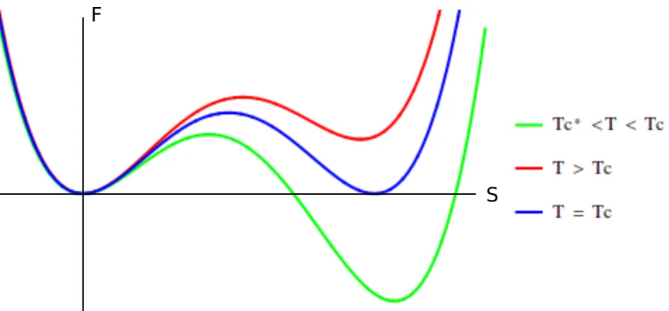
The Landau theory is a general description of phase transitions [13]. It assumes that there is an order parameter, which is zero for disordered and non-zero for the ordered state. It is based on this idea that the free energy of the system can be expanded as a power series in the order parameter. Examples of an order parameter can be regarded as electric polarization in a ferroelectric state[14], magnetization in a ferromagnetic state [15], etc. In Landau theory, a first order transition from disordered to ordered state is a transition in which the order parameter changes discontinuously from zero to a non-zero value.

(18)

1.4. Landau-deGennesTheory ofLiquidCrystals 7

transition based on Landau theory. According to this model, known as Landau de Gennes theory, the free energy of the liquid crystal can be expanded in powers of the order parameter Q as follows [7]:

F = F0+ 1

2A(T −T ∗

c)QαβQβα+

1

3BQαβQβγQγα+ 1

4C(QαβQαβ)

2₊_O₍_Q5₎_. _(1.5)

In the uniform aligned state, using 1.3, equation 1.5 becomes:

F = F0+

3A(T −Tc∗)

4 S

2₊ B 4S

3₊ 9C 16S

4₊_O₍_S5₎_, _(1.6)

where A, B, and C are constants and Tc∗ is a temperature, a little bit smaller than the critical

temperature,TC, at the transition. As the positive and negative values of the scalar parameter

correspond to different molecular alignments, the free energy must contain odd power of S, so thatF(S)_,F(−S) .

The reason for the discontinuity in the order parameter is shown in figure 1.6 . In this figure,

Figure 1.6: The Landau free energy of a nematic liquid crystal as a function of the scalar order parameter S.

(19)

(a) Bend (b) Splay

(c) Twist

Figure 1.7: Elastic distortions in liquid crystal

is the stable phase above the critical temperature. However, there is a coexistence of nematic and isotropic phases atT = Tc, and atTc∗ <T < Tc the absolute minimum in energy occurs at

a non-zero value of order parameter. This corresponds to the first order phase transition, as the order parameter, where the free energy is minimum, is changing discontinuously.

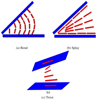
It should be emphasized that the Landau free energy is applicable to the situation in which there are no external effects acting on the nematic liquid crystal, which rarely happens. Often, to accommodate boundaries or other external effects, the director locally undergoes elastic distortions. Typically, the distortions are categorized into 3 different cases: splay, twist, and bend distortions. These cases can be seen in figure 1.7. These distortions can be described by the Frank elastic free energy [16, 17] :

Fe =

1

2K1(∇ ·nˆ) 2₊ 1

2K2(ˆn· ∇ ×nˆ) 2₊ 1

2K3(ˆn×(∇ ×nˆ))

(20)

1.4. Landau-deGennesTheory ofLiquidCrystals 9

Splay is parameterized by K1, showing an outward widening, twist is represented byK2, and bend byK3. This energy can be written in terms of the tensor order parameter as follows:

Fe =

L1

2 (∂αQβγ) 2₊ L2

2(∂αQαγ)(∂βQβγ)+ L3

2 Qαβ(∂αQγ)(∂βQγ)+ 4πL1

P αβγQαν(∂βQγν). (1.8)

L1, L2, andL3 can be mapped onto K1, K2, andK3. P is the value of pitch if the medium is a cholesteric liquid crystal [18].

In addition to the bulk energy of the liquid crystal, its interaction with surfaces must be con-sidered as well. This should be characterized by the preferred orientation of the liquid crystal, applied by the surface boundary, and the anchoring strength αs. This interaction can be

de-scribed by [1, 19]:

Fsur f ace =

αs

2 (Qi j−Q 0

i j)

2 _→

Per pendicular anchoring (1.9)

Fsur f ace =

αs

2( ˜Qi j−Q˜i j ⊥

)2 → Planar anchoring, (1.10)

where ˜Qi j = Qi j + 1₃S0δi j and ˜Qi j

⊥

= (δik − nˆi0nˆk0) ˜Qkl(δl j − nˆl0nˆj0) is the projection of ˜Qi j

onto the tangent plane of the surface. AlsoQ0_{i j} = S0( ˆni0nˆj0− 1₃δi j), and ˆn0is the normal to the

surface, andS0is the equilibrium scalar order parameter in the undistorted state.

(a) Planar (b) Perpendicular

(21)

1.5 Liquid Crystal Hydrodynamics

The evolution of the order parameter can be tracked using the Beris-Edwards formulation [20]:

(∂t +u· ∇)Q−S(W, Q)= ΓH, (1.11)

with

S(W, Q)= (ξD+ Ω)(Q+I/3)+(Q+I/3)(ξD−Ω)−2ξ(Q+I/3)T r(QW), (1.12)

whereD = (W +WT₎/_{2 and}_Ω= ₍_W ₋_WT₎/_{2 correspond to the symmetric and}

antisym-metric parts of the velocity gradient tensorWαβ =∂βuα, and the effective aspect ratio of liquid crystal molecules is described byξ, andΓ is the collective rotational diffusion constant. The right hand side of equation 1.11 drives the system towards the minimum of the free energy, and H is related to the functional derivative of the free energy:

H = −δF

δQ + I 3

!δ

F

δQ. (1.13)

As the liquid crystal is considered a fluid, it should satisfy the continuity and Navier-Stokes equations. However, the stress tensor in these equations contains the additional complexities of the liquid crystal which has both symmetric

σαβ= −P0δαβ−ξHαγ(Qγβ+ 1

3δαβ)−ξ(Qαγ+ 1

3δαγ)Hαβ +2ξ(Qαβ+ 1

3δαβ)QγHγ −∂_βQγν(_δ∂δF

αQγν),

(1.14)

and antisymmetric

(22)

1.6. TopologicalDefects 11

components.

1.6 Topological Defects

Topological defects are created when there is a local singularity in the order parameter of the system. They are observed in crystalline solids [21], superfluid helium [22], and cosmol-ogy [23].

Defect structures can exist in a liquid crystal medium as well. In fact, the name of ”nematic” liquid crystals comes from the thread-like defect, which was observed under a microscope in the medium of LC by Friedel [24]. Defects can be produced by applying a specific boundary condition at the surface in a liquid crystal. Imposing the boundary conditions creates spots within the liquid crystal where the director field changes its direction discontinuously, so these spots are considered as a singularity or discontinuity. When defects are present within the sample, the whole free energy of the system increases. Therefore, there is no defect in an ideal ordered system.The singularities can be in the form of points or lines, the later are called discli-nations.

Categorizing the defect structure involves specifying the strength of the defect, which is an in-teger or half inin-teger. In order to determine the defect strength, a closed path must be traversed counter clockwise around the defect and then the strength is obtained by finding the angle the director is rotated and dividing by 2π

m= φ

2π , m=0, ± 1

2, ±1, ... . (1.16)

(23)

(a)m=−1/2 (b)m= +1/2

(c)m=−1 (d)m= +1

(24)

1.7. ColloidalParticles 13

1.7 Colloidal Particles

If colloidal particles are present in the liquid crystal medium, due to preferred anchoring of molecules on the surface of particles, the director becomes distorted from its uniform orien-tation. Therefore, topological defects are generated around the particles [26]. It has been observed that the preferred anchoring of fluid molecules on the surface of particles is typically parallel (planar anchoring),or perpendicular (normal or homeotropic anchoring).

If the fluid molecules prefer to have tangential anchoring on the surface of the colloidal, two small radius+1₂ disclination loops are formed at the poles of spheres, called boojums. [27]. On the other hand, in the case of normal anchoring, two possible defect structures may be pro-duced. One structure can be a -1 point defect, called a hyperbolic hedgehog, located near the surface of the colloidal, as illustrated in figure 1.10.

Figure 1.10: Hyperbolic Hedgehog.

Another possibility is a disclination ring surrounding the particle which is called Saturn-ring defect, shown in figure 1.11b. The radius of the particle dictates which defect structure is generated in normal anchoring. It has been seen that the Saturn ring is the stable structure for small particles while the hedgehog point defect is produced for large particles [28, 6].

(25)

interac-(a) Boojums (b) Saturn ring

Figure 1.11: Possible defects around the colloidal particles depending on molecule anchoring on their surfaces. In a) the sphere has planar anchoring and in b) the sphere has perpendicular anchoring. The pink lines correspond to contour plot of positions around the collidal particles where the scalar order parameter drops 15% of the bulk value. In both a) and b) the director is shown at the surface of spheres.

(26)

Figure 1.12: Boojums on the surface of the colloidal particles when they get close each other along the director in nematic. [1]

away from the x-axis. As the defects become displaced from the x axis, there would be an induced attraction between the particles. This attraction is energetically favorable as the vol-ume of the distorted region reduces. So the particles with planar anchoring attract each other at close distances, while they repel when they are far from each other [1]. Generally, attracting particles, when they are close to each other, in order to minimize the elastic energy, produce self-assembled structures such as linear chains [6] and 2D crystals [32].

However, in a cholesteric liquid crystal the defect lines become twisted. These structures can be controlled by the value of pitch in the cholesteric. In both cases of planar and normal an-choring, the defect lines wind around the particle, as the pitch decreases [33]. This is illustrated in figure 1.13

(27)

the defects on adjacent particles connect to each other when they are close to each other, and a defect-bonded particles chain is generated, which is shown in figure 1.14.

(a) Pitch=1.5µm

(b) Pitch=3µm

(c) Pitch=1.5µm (d) Pitch=3µm

Figure 1.13: Defect structures around the colloidal particles in cholesteric liquid crystal

(28)

Figure 1.14: Defect-bonded chain [2]

Figure 1.15: a) Free energy as a function of their particle-particle separation b) Angular sepa-ration of defect points [2]

favorable that bonding happens.

(29)

Figure 1.16: Free energy as a function of the angular positioning of the particles relative to the twist axis [2]

other. As a result, this compensates for the longer defect lines as they are pulled apart and there is a quadratic dependence of free energy vs. particle separation. When particles are moved out of plane (so one particle is at a different part of the background twist in the cholesteric), as seen in figure 1.16, it can be seen that defect bonding still happens for 0< θ <25◦. However, the bond breaks at about 25◦ _{and the energy levels o}_ff_for_{θ >} _{25. It also shows that there is} a preference for alignment in a plane perpendicular to the twist axis, since the free energy is minimized atθ=0.

(30)

Chapter 2 Methodology

2.1 Introduction

One of the computational methods to describe the motion of particles, at the microscopic level, is molecular dynamics (MD). In this approach, Newton’s equation of motion for each individ-ual particle is solved to track the trajectories of particles [34]. On the other hand, the fluid can be regarded as a continuous medium at the macroscopic level, in which the Navier-Stokes and continuity equations [35] are solved to evaluate the fluid flow. Navier-Stokes equations are partial differential equations which can be solved by a variety of methods, such as finite difference methods [36].

Each of these two methods has its own difficulties. At the macroscopic level, the potential numerical instability of methods to solve complicated non-linear partial equations is a problem that is a concern that can limit the size of the timesteps. Also, these numerical methods in-volve discretization of the equations and truncation errors which raise the question of whether physical quantities are conserved or not [37]. On the other hand, considering the system with colloidal particles immersed in the fluid, the MD algorithm is an impractical approach to sim-ulate the motion of fluid molecules as the solvent, since the majority of the particles consists of solvent. Therefore, tracking the position of a large number of individual fluid particles costs

(31)

time and computer resources.

As a result, one considers a mesoscopic level, which is between the microscopic and macro-scopic level [38]. One of the common and popular methods at this level, is the lattice Boltz-mann method, which evaluates the collective behavior of fluid particles based on a collision procedure and does not involve solving Navier-Stokes and continuity equations directly. In this chapter, this method is described for a simple fluid and then generalized to model the motion of a liquid crystal.

2.2 Lattice Boltzmann Method: Historical Background

The lattice gas cellular automata is often described as the historical origin of lattice Boltzmann methods. In lattice gas automata, introduced by Hardy, Pomeau, and de Pazzis (HPP), the terms “lattice”and “gas”imply a gas is moving on a lattice, and “automata”suggests a set of rules governing the evolution of the gas. In this method, boolean particles (0 or 1) are used to represent the gas. Further, the fluid is regarded as a set of particles present on a square lattice with discrete velocities, and each step involves collision and streaming of particles [39]. How-ever, the motion of particles does not satisfy Navier-Stokes equations in the long wavelength limit, which is considered one of the deficiencies of this method. This problem is due to the insufficient degree of rotational symmetry of the square lattice, which does not generate an isotropic lattice tensor (composed of moments of lattice vectors) [40, 37].

The correct form of Navier-Stokes equation in the long wavelength limit can be produced by using a hexagonal lattice, which has enough symmetry to reproduce Navier-Stokes equation, as shown by Frisch, Hasslachor and Pomeak [41]. Their FHP model is similar to the HHP model, but involves more collision rules due to its hexagonal symmetry [37]. This model still suffers from some drawbacks such as the existence of large statistical noise due to boolean variables, velocity dependence of fluid pressure, and a few other problems.

(32)

Boltz-2.3. TheBoltzmannEquation 21

mann method (LBM). In this method the discrete particles are replaced by distribution func-tions to reduce the statistical noise. The LBM has been popular and successful in a variety of fields such as quantum mechanics [42], magnetohydrodynamics [43], and solving the diffusion equation [40].

2.3 The Boltzmann Equation

As the basic idea of LBM is replacing the discrete particles by particle distribution functions, this method can be explained through kinetic theory. This theory deduces the macroscopic properties of a large number of particles such as pressure, temperature, energy, etc, based on the Hamilton’s equation of motion of particles:

∂H

∂pi

= dxi

dt ,

∂H

∂xi

=−dpi dt ,

(2.1)

where H is the Hamiltonian. In a system of N particles, if the positionxiand momentumpiof

all the particles are specified, then the micro-state of this system can completely be determined, corresponding to a point in phase space, a space where the coordinates are given by position and momentum vectors, and time [44].

Following the statistical approach, the single-particle distribution f(x,p,t) can be introduced in a way that f(x,p,t)d3_xd3_p_{gives the total number of particles positioned in a range between} xand x+d3_x_{and momentum in the range between} _p_and_p+_d3_p_{. Assuming there are no} collisions existing in the system, if an external force is applied to a particle, then the single particle distribution function, before and after applying the force, satisfies [45]:

f(x+ p

(33)

This type of evolution is referred to as streaming. But, the number of particles can differ from its value predicted by simple streaming if collisions occur between the particles. In this case, some particles can be added to, or removed from the small volume. So, the evolution of the distribution of the number of particles can be written as:

f(x+ p

m∆t,p+F ∆t,t+ ∆t)− f(x,p,t)= ψ12∆t, (2.3)

whereψ12is the rate of change between final and initial distribution function due to collisions, and is called the collision integral. Using a Taylor expansion of f(x+ p_m∆t,p+F ∆t,t+ ∆t),

f(x+ p

m∆t,p+F ∆t,t+ ∆t)= f(x,p,t)+

∂f

∂x · p m∆t+

∂f

∂p · F ∆t+

∂f

∂p∆t+... . (2.4)

Now the Boltzmann equation can be written as:

"∂ ∂t +

p m ·

∂

∂x +F ·

∂ ∂p

#

= ψ12, (2.5)

where the left hand side is equal to the material derivative of f(x,p,t) which we denote by Dtf(x,p,t) and call the streaming term, while the right hand side is the collision integral. The

collision integral has the following form, assuming the particles are completely uncorrelated prior to a collision [44, 46]:

ψ12 = 1 m

Z

d3p2dΩ|p2−p1 |σ(Ω) [f(x1,p01,t)f(x1,p02,t) − f(x1,p1,t) f(x1,p2,t)],

(2.6)

(34)

2.4. LatticeBoltzmannMethod 23

fact, f(x₁,p₁,t) f(x₁,p₂,t) indicates the loss of particles taken out, and f(x₁,p0

1,t)f(x1,p02,t) describes the gain of particles taken indx3_dp3 _[40].

In many cases, the Boltzmann equation can be simplified using the BGK(Bhatnagar-Gross-Krook) collision operator [47]:

ψ12 =−

f − feq

τ , (2.7)

which indicates that collisions tend to relax toward an equilibrium distribution function feq, and the time scaleτcan be regarded as the “collision time”. The equilibrium distribution function corresponds to a Maxwell-Boltzmann equation [44].

The macroscopic quantities can be obtained by calculating the moments of distribution function f(x,p,t):

Z

f(x,v,t)d3v = ρ ,

Z

f(x,v,t)vαd3v = ρuα,

(2.8)

whereρis the fluid density anduαis the fluid velocity.

2.4 Lattice Boltzmann Method

The lattice Boltzmann equation can be obtained directly from the continuous Boltzmann equa-tion by discretizing time, space, and velocity [48]. So the discretized Boltzmann equaequa-tion can be written as:

fi(xα+eiα∆t,t+ ∆t)− fi(xα,t) = −

∆t

τf

(fi(xα,t)− f eq

(35)

where pi is a forcing term, ei is a discrete velocity vector, and fi is the partial distribution

corresponding toei.

Analogous to 2.8 we have:

X

i

fi ≡ρ ,

X

i

fiei ≡ρuα.

(2.10)

In LBM, equation 2.9 is solved on a lattice. At each node of the lattice, the particle distributions move along the specified velocity direction to the neighboring nodes. The lattice Boltzmann equation can also reproduce the continuity and Navier-Stokes equations in the long wavelength limit [38]. The number of directions is indicated by the lattice configuration. These configura-tions can be determined by the dimension of the problem and the number of velocity direcconfigura-tions which is labeled by DnQm, where n refers to the dimension and m indicates the number of

velocity directions. Typical cases are illustrated in figure 2.1. In 2D, the common model is D2Q9, and the velocity directions are:

e0 =(0,0) , e1= (1,0) , e2 = (0,1),

e3 =(−1,0) , e4 =(0,−1) , e5 =(1,1), e6 =(−1,1) , e7 =(−1,−1) , e8= (1,−1).

In 3D,D3Q15is used as a common model :

e(0)_i = (0,0,0),

e(1)_i = (±1,0,0),(0,±1,0),(0,0,±1), e(2)_i = (±1,±1,±1),

(36)

2.4. LatticeBoltzmannMethod 25

(a)D₂Q₉ (b)D₃Q₁₅

Figure 2.1: Different lattice configuartions

The following equations are used to constrain the equilibrium distribution and to control the stress tensor:

X

i

f_ieq = ρ ,

X

i

f_ieqeiα = ρuα,

X

i

f_ieqeiαeiβ= −σαβ+ρuαuβ.

(2.11)

The continuous equilibrium distribution function is the Maxwell-Boltzmann distribution which has the following form in 3-dimensions:

feq =ρ( m 2πkBT

)32exp(−m(v−u) 2

2kBT

),

= ρ( m 2πkBT

)32exp(− mv 2

2kBT

)exp(m(v·u) kBT

− mu 2

2kBT

)

| {z }

*

(37)

Then the indicated function can be expanded in a Taylor series as follows with small velocity:

feq = ρ( m 2πkBT

)D2_exp₍− mv 2

2kBT

)

1+(m(v·u) kBT

− mu 2

2kBT

)+ 1 2(

m(v·u) kBT

− mu 2

2kBT

)2]+...

=ρ( m 2πkBT

)32exp(− mv 2

2kBT

)

1+ m(v·u) kBT

− mu 2

2kBT

+ 1 2

m(v·u) kBT

2+

O(u3)],

(2.13)

whereρ(_2πm_k

BT) D

2exp(−mv 2

2kBT) is related as the weight function. Therefore, the general discretized

form of the equilibrium distribution function, using discrete weightswiassociated with each of

velocity directions, can be given as follows [49, 48]:

f_ieq = ρwiA+Buαeiα+Cu2+Duαuβeiαeiβ+Eαβeiαeiβ]. (2.14)

The constants can be obtained by the above constraints, and the weighting coefficients are given as [37]:

D2Q9 →wi =

                  

4/9 i=0 1/9 i=1, ...,4 1/36 i=5, ...,8

,

D3Q15 →wi =

                  

2/9 i=0 1/9 i=1, ...,6 1/72 i=7, ...,14

.

It should be taken into account that this method is only valid for an incompressible fluid, mean-ing the density of fluid is not varied significantly.

To sum up, the Boltzmann equation is solved in 2 steps: -Collision step:

fi(xα,t+ ∆t)= fi(xα,t)−

∆t

τf

(fi(xα,t)− f eq

(38)

2.5. Modeling aLiquidCrystalThroughLBM Algorithm 27

which indicates that the distribution function tends to relax towards the equilibrium distribution function.

-Streaming step:

fi(xα+eiα∆t,t+ ∆t)= fi(xα,t+ ∆t), (2.16)

showing the particles are moving from one site to the neighboring site.

2.5 Modeling a Liquid Crystal Through LBM Algorithm

So far, LBM has been described only for a simple fluid, which is defined in terms of a single set of particle distribution functions, the scalar fi(x). As liquid crystal hydrodynamics involve the

evolution of a tensor order parameter, a second set of distribution functions, the tensorsGi(x)

which are related to the tensor order parameterQ[20, 50] must be considered as well. Again Gi corresponds to a lattice vectorei. Here, we work on a cubic lattice with theD3Q15 model, which was described in previous sections.

The order parameterGialso evolves as :

Gi(xα,t+ ∆t)−Gi(xα,t)= −

∆t

τG

(Gi(xα,t)−G eq

i (xα,t))+Mi∆t, (2.17)

whereMi is a forcing term. The first moment ofpi control the antisymmetric part of the stress

tensor:

X

i

pi = 0,

X

i

pieiα= ∂βταβ,

X

i

pieiαeiβ =0. (2.18)

Now the moments of the equilibrium order parameter distribution can be chosen as :

X

i

Geq_i =Q, X

i

Geq_i eiα =Quα,

X

i

(39)

Also, the forcing term satisfies :

X

i

Mi = ΓH(Q)+S(W,Q),

X

i

M_ieqeiα =

X

i

Mi

uα. (2.20)

Now, both equilibrium distribution functions and forcing terms can be written as polynomial expansions in velocity:

f_ieq =As+Bsuαeiα+Csu2+Dsuαuβeiαeiβ+Esαβeiαeiβ,

Geq_i = Js+Ksuαeiα+Lsu2+Nsuαuβeiαeiβ,

pi =Ts∂βταβeiα,

M =Rs+Ssuαeiα,

(2.21)

wheres∈ {0,1,2}indicates the coefficients for vectorses

i. By using the constraints 2.11, 2.18,

2.19, and 2.20, all the coefficients can be determined as follows [20]:

A2 =− 1 10

T r1 3σ

, A1 = A2, A0 =ρ−14A2,

B2 = 1

24ρ, B1 = 8B2, C2= −

1

24ρ, C1 =2C2 C0= − 2 3ρ, D2 =

1

16, D1 =8D2, E2αβ = 1

16

−σ+T r1 3σ

δαβ

, E1αβ =8E2αβ

J0 =Q, K2 = 1

24Q, K1 =8K2 L2 =−

1

24Q, ,L1 =2L2, L0 =− 2 3Q N2=

1

16Q, N1 =8N2, R2 =

1 15

ˆ

H, R1 =R0= R2,

S2 = 1 24

ˆ

H, S1 = 8S2,

T2 = 1

24, T1 =8T2

(40)

2.6. CoupledLB-MD Method 29

2.6 Coupled LB-MD Method

In order to model a system of colloidal particles immersed in a liquid crystal, as mentioned previously, LBM is an efficient method to simulate the motion of a large number of liquid crys-tal molecules as solvent. In addition, a MD algorithm is used to model the motion of colloidal particles based on solving Newton’s equations of motion. Therefore, these two methods are combined to model the whole system. The coupled LBM and MD algorithm have a lot of applications such as polymers in solution [51], colloidal suspensions [52].

2.6.1 Particle-Fluid Interaction

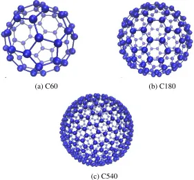
In our work, the colloidal particles are considered as spherical objects, and must be mapped onto the computational fluid mesh. In order to couple the object to the fluid lattice, the surface of the object must be discretized into a set of nodes and each node behaves as an individual MD particle, as shown in figure 2.2.

(a) C60 (b) C180

(c) C540

(41)

Figure 2.3 shows a finite object in two dimension. According to this figure, the finite object is interpolated on the fluid mesh and its surface nodes are distributed to the corners of the lattice site where they exist by assigning the ratioξαj of the opposing area to the total area of

the lattice cell to the corresponding mesh site [53]. As we work in three dimension, the ratio of areas are replaced by volumes: ξαj = φj(xα)φj(yα)φj(zα). Figure 2.2 shows some examples

of spherical objects which are discretized by a set of nodes. This method is called the trilinear interpolation method, or trilinear stencil and the weights assigned to each of the nearest lattice sites is [54, 55]:

φj(rα)=1− |∆r|, (2.23)

where∆r = rα−rj

∆x . Here, the position of the fluid mesh site is labeled byrj, the position of the

node is labeled byrα, and the lattice spacing is indicated by∆x. Now the interaction between the object and fluid must be considered by applying the forces to particle nodes and fluid mesh sites. So the force exerted on a lattice site jdue to particle nodeαis:

Fjα =γ(vn−uf)ξjα (2.24)

Figure 2.3: P1 is affected by node i by the ratio 0f ₍_∆A_X1₎2

(42)

2.6. CoupledLB-MD Method 31

particle node location andvnis the particle velocity.

Now the total force applied to the fluid by the node α can be calculated as γ(vn − uf), as

P

jξjα = 1. According to Newton’s third law, there is an equal and opposite force applied to

particle nodeα:

Fα = −γ(vn−uf). (2.25)

Through the elastic collision between the particle nodes and mesh sites in discrete time, it can be shown thatγis calculated as [55],

γ= 2mumv

mu+mv

1

∆tcoll

, (2.26)

where ∆tcoll is the time of collisions between the fluid and particles, mv is the particle mass,

andmu is the representative mass fluid on the particle node. As τindicates the time between

the collisions in the fluid, it can be assumed that the collision time between fluid and particles is equal to the fluid relaxation time_∆τ_t =1

In order to calculate the contribution of surface energy due to the applied boundary conditions on the surface of particles, an area per node, which can be determined by dividing the total surface of spherical particles by the total number of their nodes, must be found, and then interpolated to each nodes’ nearest lattice sites as follows:

∆A

j =

X

α ∆A

αξjα, (2.27)

where ∆A

α = 4πR2/number of the nodes, and ∆Aj is the interpolated of area per node on

the lattice site j,and R is the radius of spherical particles. Using 1.10 and 1.9, the surface energy interpolated on the mesh site j can be calculated as :

Fsur f ace_j =

αs

2 (Qlm−Q 0

lm)

2 _∆ A

j → Per pendicular anchoring. (2.28)

Fsur f acej =

αs

2( ˜Qlm−Q˜ ⊥

lm)

2₍_∆_A

(43)

2.7 Summary

(44)

Chapter 3 Results

So far, studies have been focused on the defect structures, and interactions, produced by col-loidal particles with the same kind of boundary conditions on their surfaces, such as the defect-bonded chain generated by colloidal particles with planar anchoring inside a cholesteric liquid crystal [2]. As many semiconductors are composed of two different elements and are consid-ered as compound materials such as GaAs or InSb, we are motivated to investigate compound colloidal structures in order to search for potential photonic materials. Therefore, in the fol-lowing chapter, we mainly investigate possible induced interactions between particles with different sorts of anchoring on their surfaces in both nematic and cholesteric liquid crystals. At the first step, we consider two spherical colloidal particles with a radius of 0.625µm in a ne-matic liquid crystal inside a simulation box with dimensions ofLx×Ly×Lz. There are periodic

boundary conditions imposed in the x and y directions, and fixed walls located in the z direc-tion, and the liquid crystal molecules are set to be parallel on the walls as shown in the figure 3.1. In our work, we use planar anchoring on the surface of one of the spherical particles, and perpendicular anchoring on the surface of the other one. The distance between the particles and the boundaries are large enough to reduce the effect of the boundaries on the particles, and the particles are put in the XY plane atz= Ly

2.

(45)

Figure 3.1: Schematic of our system where the periodic boundary conditions are imposed in the x and y directions, the fixed walls are located in the z direction, and the liquid crystal molecules are set to be parallel on the walls.

Here, we have chosen the one elastic constant approximation as K1 = K2 = K3. The con-stants A, B, and C, used in the bulk free energy, are chosen as: A = A0

2(1− γ

3) ,B = A0 γ 3 , and C = A0γ₄. The value ofγ controls the transition from isotropic to liquid crystal phase,γ > 2.7 corresponds to the nematic phase. All the simulation parameters are shown in table 3.1. As described in the previous chapter, the surface of colloidal particles must be discretized into a set of nodes to be coupled to the computational mesh of the liquid crystal. In our work, all the particles are discretized into 540 nodes. The simulation of these particle nodes in the liquid crystal is performed in the open source molecular dynamics package, LAMMPS, and integrated through the verlet-velocity algorithm; however, we freeze the particle nodes in the simulation by setting the forces to zero, so they are not allowed to move. This way we can investigate the equilibrium energy at many different spacings and orientations.

(46)

3.1. IndividualSpheres inNematic 35

implemented for a total of 30000 timesteps, and the total number of simulations that we per-formed was about 440. Each job used 16 processors and took 2 days to be completed.

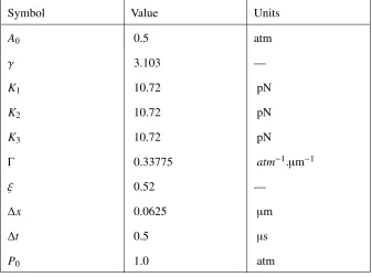
Table 3.1: Parameters

Symbol Value Units

A0 0.5 atm

γ 3.103 —

K1 10.72 pN

K₂ 10.72 pN

K3 10.72 pN

Γ 0.33775 atm−1.µm−1

ξ 0.52 —

∆x 0.0625 µm

∆t 0.5 µs

P₀ 1.0 atm

3.1 Individual Spheres in Nematic

Before considering two spheres, the defect structures of each of the individual spheres were investigated separately. Figure 3.2 shows the defect structure for planar and perpendicular anchoring for isolated spheres in a nematic. In this figure, the pink lines correspond to defects, and show a contour plot of the positions around the particles where the scalar order parameter has decreased about 15% from the bulk value.

(47)

structures around the particles in a liquid crystal and charges in electrostatics. As the director field satisfies the linear Laplace’s equation far from the colloidal particles, where deviations from uniformity are small [6, 7], it can be concluded that it is analogous to electrostatics in which the electrostatic potential satisfies Laplace’s equation as well. Therefore, the defects in liquid crystal can be analogous to electric charges in electrostatics.

(a) Boojums (b) Saturn-ring

(c) The image of boojums (d) The image of ring

Figure 3.2: The defects and their images for isolated particles in a nematic liquid crystal. In (a) and (c) the sphere has planar anchoring and in (b) and (d) the sphere has perpendicular anchoring. The director is shown on the surface of the sphere in (a) and (b) and the sphere is not shown in (c) and (d), so that the image defects are visible.

3.1.1 Interaction of Two Particles Immersed in a Nematic Liquid Crystal

(48)

3.1. IndividualSpheres inNematic 37

one, and located at different distances with respect to each other. The angles are measured with respect to the x axis. In this case, completely new defect configurations have been observed. As can be seen in 3.3, while the sphere is being rotated, the defect lines between the particles get connected to each other at about 35◦ _{and become disconnected at} θ _≥ ₃₉◦_{. This kind of} behavior can be seen up to a specific separation of about 0.375µm. The defect lines do not connect to each other at larger distances.

The interaction of these particles can be explored through a 2D and 3D contour of the interac-tion energy of system. As is shown in figure 3.4, the energy is maximized atθ ∼ 35◦, where the defect lines are joined together, and there is a minimum atθ∼ 90◦at small particle-particle separations.

(49)

3.5, which is the plot of director field around the particles, shows that there is a slightly higher distorted volume around the particles at this angle. Therefore, the particles tend to repel each other at 35◦ to prevent increasing the distortion in the medium. On the other hand, when the particles are close to each other at θ ∼ 90◦_{, the plot of the director field indicates a less} dis-torted region exists between the particles. As a result the particles prefer to become attracted to this position. There is also another local minimum atθ ∼ 0◦ _{and at a distance of 0}.₁₂₅µ_m, indicating an attraction between the particles.

3.2 Interaction of Particles Immersed in a Cholesteric

Liq-uid Crystal

Now the medium is switched from nematic to cholesteric liquid crystal. As the properties of a cholesteric liquid crystal can be dependent on the value of its pitch, several pitch values have been tried to measure the interaction energy. The values that were selected, 1.5 µm, 3 µm, and 1.125 µm, are close to the size of the particle, larger and smaller than the particle size, respectively.

(50)

3.2. Interaction ofParticlesImmersed in aCholestericLiquidCrystal 39

(a)θ=0◦

(b)θ=15◦ (c)θ=25◦

(d)θ=30◦ (e)θ=32◦ (f)θ=35◦

(g)θ=37◦ (h)θ=39◦ (i)θ=43◦

(j)θ=45◦ (k)θ=55◦ (l)θ=60◦

(m)θ=85◦ (n)θ=90◦

(51)

(a)

(b)

(52)

(a)θ=35◦

(b)θ=90◦

(53)

lines of both particles are joined together. Atθ ∼ 60◦, the defect lines are only connected on one side. The most fascinating defect structure happens atθ∼85◦. At this position, the defect lines are connected not only on both sides, but also at two points in the middle of the particles, which looks like a symmetric defect structure. Atθ∼ 90◦_{, this symmetric defect model is not} seen.

Next, the particle-particle separation is increased to 0.25µm with the same value of pitch, shown in figure 3.7. Atθ = 0◦, the defect lines of boojums and Saturn ring are shared in the middle of particles. At larger angles, they are connected at both sides again, and at θ ∼ 37◦ , the ring gets connected in the middle as well. Atθ ≥ 43◦, they become disconnected at one side, while joined at one common point on the other side.

In figure 3.8 and 3.9, when the particles are separated 0.375µm from each other, no defect lines are connected between the particles up toθ ∼ 43◦_{. At} θ _∼ ₄₃◦ _{the defect lines are connected} at two points at one side of the particles. Atθ ≥ 55◦_{, the lines are not joined at any points but} there is a connection of defect lines at one side and in between the spheres. Furthermore, at

θ ∼ 90, there is one point where the defects are connected as well. At a separation of 0.5µm,

no connection occurs, while the boojum defect lines become different in shape at θ ∼ 60◦, as is exhibited in figure 3.10. At larger separations, no defect lines are joined together. In the plot of the interaction energy of particles, figure 3.11, there is a sharp maximum in energy at

θ∼ 90◦_{, where the particles are separated about 0.375}µ_{m from each other and the defect lines}

are joined at one common point at one side and there is a defect line connected to other sphere which is passed in between the particles. It seems that the defect lines get more stretched at this specific configuration, so it can be concluded that the total length of defect lines is higher than other positions, which leads to increase in the energy. So there is a repulsion when the particles approach each other from far distances.

(54)

(a)θ=0◦ _(b)_θ₌₁₅◦

(c)θ=25◦

(d)θ=32◦ (e)θ=35◦ (f)θ=55◦

(g)θ=60◦ (h)θ=85◦ (i)θ=90◦

(55)

(a)θ=0◦ _(b)_θ₌₁₀◦ _(c)_θ₌₃₀◦

(d)θ=35◦ (e)θ=37◦ (f)θ=43◦

(g)θ=60◦ (h)θ=75◦ (i)θ=90◦

(56)

(a)θ=0◦ _(b)_θ₌₃₇◦ _(c)_θ₌₄₃◦

(d)θ=45◦ (e)θ=55◦ (f)θ=75◦

(g)θ=90◦

(57)

(a)θ=43◦ _(b)_θ₌₄₅◦

(c)θ=55◦

(d)θ=75◦ (e)θ=90◦

(58)

(a)θ=0◦ (b)θ=25◦ (c)θ=45◦

(d)θ=60◦ (e)θ=75◦ (f)θ=90◦

(59)

(a)

(b)

(60)

The same sort of structure is observed up to the specific particle separation of 0.375µm. So it seems the defect structure in cholesteric liquid crystal with higher value of pitch looks similar to the defects in nematic. As it can be seen in figure 3.13, the interaction energy is maximized at about 15◦₋₂₅◦_{, corresponding to the configurations where the defect lines start} to be connected to each other in between the particles, so the particles tend to repel each other, as the distortion of director field between the particles increases at this configuration. Also there is a minimum in energy when the particles are very close to each other at θ ∼ 90◦. In this case, like the particles inside a nematic, there is a lower distorted volume in between the particles, which makes them attract each other.

Next, the defect structures and interaction of two particles is investigated in a cholesteric with the lower pitch value of 1.125µm. In this case, the defect lines are much more twisted around the particles. Figure 3.14 and 3.15, show the defect structure of particles when they are kept at a distance of 0.125µm. Atθ ∼ 0◦_{, two twisted defect lines are joined together from both} sides and a defect in a shape of handle appears on the surface of the particle with planar an-choring. Atθ= 25◦, the Saturn ring starts to join to the mentioned handle defect, so the defect in between the particles does not look like a handle any more. If we look at the particle at

θ = 30◦, it can be recognized that the twisted line is surrounding the particles and the Saturn ring gets connected to the surface of the other particle in between. This structure is seen up to

θ=45◦_{. At this angle, there is a point on one side of particles, where the defect lines are joined}

(61)

µm, seen in figure 3.18 and 3.19, the same sort of defects are seen but at different values of

angles. At 0 ≤ θ <55◦, there is a defect line surrounding the particles. Atθ ∼ 55◦, again we see a point where the defect lines are joined at one side and the symmetric defect structure is observed at 75≤ θ≤90◦_{. There is no connection in defect lines for larger distances.}

If we look at the plots of the energy of the particles, as shown in figure 3.20, we see that the interaction energy increases atθ >∼ 55◦_{at a particle separation of about 0}.₂₅µ_{m, in which the} defect lines get connected between the particles as well and the total length of lines is higher, leading to increase the distortion volume. This indicates that there is a repulsion between the particles when they approach each other from further distances. Also the energy is minimized atθ ∼ 0◦when they are close to each other, as there is a less distorted volume in the medium. So the particles become attracted to this position.

So far the spheres have been confined on the XY plane. Now, the next step is investigating the possible induced interactions between the particles, with produced defect structures, when they are rotated only on the XZ plane and the spheres are located aty= Ly

2.

(62)

Next, the particles are placed into a cholesteric with pitch value of 1.5µm. Figure 3.24 shows the defect structures of two particles when they are separated by 0.125µm from each other. At

θ = 0◦, we see that the boojums and the Saturn ring are joined together into one defect line, which is surrounding both particles. Atθ = 15◦_{, the defect lines get disconnected at one side} of the particles; however, they are joined in between. Moreover, the ring and the boojums are connected to each other at two points at one side of particles at θ = 30◦_{. At} θ = ₃₇◦_{, there} is only one point where they are joined together. Also, no connection happens in between the particles atθ= 45◦. Atθ=60◦the defect lines are joined from both sides and the boojums get connected to the ring at the pole of particle with perpendicular anchoring. No defect lines are joined together for greater angles. This kind of behavior is not seen for particles separations greater than 0.25µm.

As it can be seen in figure 3.25, the energy is maximized atθ ∼ 15◦_{, while it is minimized at}

θ ∼ 60◦_{. This can be described by considering this point that the defect lines start to connect}

to each other at two points in between the particles at θ ∼ 15◦; however, the defect lines are twisted in a way that no extra defect appears in between the particles atθ∼ 60◦. So they prefer to repel each other atθ∼15◦, while there is an attraction between the particles atθ∼60◦ . Now, it is worthwhile to compare the results obtained for both XY and XZ planes. If we focus on the interaction energy of particles, we recognize that its total range in the nematic liquid crystal, on both XY and XZ plane, is much lower than the cholesteric liquid crystal. Moreover, if we compare the particles, for nematic medium, placed on the XY plane and the XZ plane, we notice that the lowest minimum in energy occurs on the XY plane rather than the XZ plane. Therefore, it can be concluded that the minimum in energy may be in XY plane for particles inside a nematic liquid crystal.

(63)

of the energy happens for a pitch value of 3µm. As a result, most probably the minimum in energy is located on the XY plane for cholesteric liquid crystals as well.

(a)θ=0◦ _(b)_θ₌₁₅◦ _(c)_θ₌₂₅◦

(d)θ=30◦ (e)θ=37◦ (f)θ=43◦

(g)θ=55◦ (h)θ=60◦ (i)θ=90◦

(64)

(a)

(b)

(65)

(a)θ=0◦ _(b)_θ₌₂₅◦ _(c)_θ₌₃₀◦

(d)θ=35◦ (e)θ=45◦ (f)θ=60◦

(g)θ=75◦ (h)θ=90◦

(66)

(a)θ=25◦ (b)θ=30◦ (c)θ=35◦

(d)θ=45◦ (e)θ=60◦ (f)θ=75◦

(67)

(a)θ=0◦ (b)θ=10◦ (c)θ=15◦

(d)θ=25◦

(e)θ=45◦ (f)θ=55◦

(g)θ=75◦ (h)θ=85◦ (i)θ=90◦

(68)

(a)θ=0◦ (b)θ=10◦ (c)θ=15◦

(d)θ=25◦ (e)θ=45◦ (f)θ=55◦

(g)θ=75◦ (h)θ=85◦ (i)θ=90◦

(69)

(a)θ=0◦

(b)θ=35◦ (c)θ=55◦

(d)θ=60◦ (e)θ=75◦ (f)θ=90◦

(70)

(a)θ=55◦ (b)θ=60◦ (c)θ=75◦

(d)θ=90◦

(71)

(a)

(b)

(72)

(a)θ=0◦ (b)θ=30◦ (c)θ=60◦

(d)θ=90◦

(73)

(74)

(a) 0.125µm

(b) 0.5µm

(75)

(a)θ=0◦ (b)θ=15◦ (c)θ=30◦

(d)θ=37◦ (e)θ=45◦ (f)θ=60◦

(g)θ=90◦ (h)θ=75◦

(76)

3.3. Discussion 65

Figure 3.25: 2D contour plot of interaction energy of 2 particles in the cholesteric LC(pitch=1.125µm)

3.3 Discussion

(77)

(78)

Chapter 4 Conclusions

In the preceding thesis, we have investigated the possible anisotropic interactions induced by defect structures around colloidal particles inside both nematic and cholesteric liquid crystals. This work was done using the lattice Boltzamnn method to model the liquid crystal and trilin-ear interpolation to couple the particles to the computational liquid crystal mesh.

In the first chapter, the liquid crystal mesophase is described, as well as its different classes such as nematic and cholesteric. As liquid crystals show anisotropic behavior and are more or-dered than an isotropic fluid, the tensor order parameter is introduced to distinguish these two phases. Then Landau de Gennes theory was presented to describe the free energy of the sys-tem in terms of the order parameter. After emphasizing the hydrodynamics equations of liquid crystals, the topological defects were described, which are generated when colloidal particles are present inside the liquid crystal. These defect structures induce anisotropic forces between the particles, which do not exist in a simple fluid such as defect-bonded chains produced by particles with planar anchoring in a cholesteric liquid crystal.

In chapter 2, the method of coupling the particles onto the lattice Boltzmann fluid is presented. In this method, the surface of a particle is discretized to a set of nodes, and the fluid is consid-ered as a computational mesh; therefore, the particle nodes are distributed onto the fluid mesh using an interpolating scheme. It is worthwhile to mention that the particle distribution

(79)

tion fi and the distribution function for the tensor order parameterGi are used in this method.

Moreover, the fluid coupling involves conservative forces based on the assumption of elastic collisions between the particle nodes and the interpolated fluid mass at the position of the par-ticle.

In chapter 3, we have investigated the interaction of two particles with different sorts of an-choring, planar and perpendicular, in both nematic and cholesteric liquid crystals. Considering the defect structures of particles separately, we see that there is an image of the outer defect lines inside the particles, which can be justified by the analogy of electrostatics, in which the potential satisfies the Laplace’s equation and liquid crystal, in which the director field satisfies the Laplace’s equation in a linearized limit as well.

First the interaction of two particles was explored when they are put in a nematic, confined on the XY plane, and one of the particles is rotated around the another one at different dis-tances with respect to each other. In this case, there is a maximum in the interaction energy when θ ∼ 35◦, corresponding to the configuration where the defect lines are joined together from both particles, so the particles experience repulsion at this configuration and the energy is minimized whenθ ∼ 90◦, where the distorted region inside the nematic has the least volume, indicating an attraction between the particles.