Scholarship@Western
Scholarship@Western
Electronic Thesis and Dissertation Repository
8-22-2016 12:00 AM
Automated Impact Crater Detection and Characterization Using
Automated Impact Crater Detection and Characterization Using
Digital Elevation Data
Digital Elevation Data
Ian M. Pritchard
The University of Western Ontario
Supervisor Dr. Jinfei Wang
The University of Western Ontario Joint Supervisor Dr. Phil Stooke
The University of Western Ontario
Graduate Program in Planetary Science
A thesis submitted in partial fulfillment of the requirements for the degree in Master of Science © Ian M. Pritchard 2016
Follow this and additional works at: https://ir.lib.uwo.ca/etd
Part of the Remote Sensing Commons
Recommended Citation Recommended Citation
Pritchard, Ian M., "Automated Impact Crater Detection and Characterization Using Digital Elevation Data" (2016). Electronic Thesis and Dissertation Repository. 3982.
https://ir.lib.uwo.ca/etd/3982
This Dissertation/Thesis is brought to you for free and open access by Scholarship@Western. It has been accepted for inclusion in Electronic Thesis and Dissertation Repository by an authorized administrator of
Impact craters are used as subjects for the remote study of a wide variety of surface
and subsurface processes throughout the solar system. Their populations and shape
characteristics are collected, often manually, and analysed by a large community of
planetary scientists. This research investigates the application of automated methods
for both the detection and characterization of impact craters on the Moon and Mars,
using machine learning techniques and digital elevation data collected by orbital
spacecraft. We begin by first assessing the effect of lunar terrain type variation on
automated crater detection results. Next, we develop a novel automated crater
degradation classification system for martian complex craters using polynomial profile
approximation. This work identifies that surface age estimations and crater statistics
acquired through automatic crater detection are influenced by terrain type, with unique
detection error responses. Additionally, we demonstrate an objective system that can
be used to automate the classification of crater degradation states, and identify some
potential areas of improvement for such a system.
Keywords: automated crater detection, Chebyshev polynomials, degradation, digital elevation model, impact crater, machine learning, Mars, Moon, profile approximation, topography
I would like to first acknowledge my supervisors Dr. Jinfei Wang and Dr. Phil Stooke
for their guidance in forming my research topics, editing this work, and sharing their
respective expertise with me. It has been a great pleasure learning from and working with
them over the course of my MSc, and I am fortunate to have found them as supervisors.
I would also like to thank Dr. Livio Tornabene, Dr. Gordon Osinski and Dr. Catherine
Neish as well as the other members of CPSX for helping me learn more about impact
cratering and remote sensing, and for providing unique opportunities to get involved in
space exploration activities.
Additionally, I’d like to thank my GITA lab mates and CPSX colleagues for
collectively helping me push forward, and providing support and stimulating
conversation. I also owe a debt of gratitude to the planetary science community as a
whole. Their tools and general philosophy of open science were instrumental parts of
my progress.
Finally, I’d like to thank my family and loved ones, who did years and years of work
to support me before I could even begin to write chapter one.
Abstract ii
List of Figures ix
List of Tables xvi
List of Appendices xviii
List of Abbreviations, Symbols, and Nomenclature xix
1 Introduction 1
1.1 Impact Cratering . . . 1
1.2 Crater Chronology . . . 4
1.3 Research Objectives . . . 7
1.4 Thesis Organization . . . 8
Bibliography 9 References 10 2 Crater Detection and Terrain Type 13 2.1 Introduction . . . 13
2.1.2 CDA Accuracy . . . 15
2.1.3 Purpose . . . 16
2.2 Methods . . . 17
2.2.1 Overview . . . 17
2.2.2 Study Areas and Data . . . 20
Study Area 1 - Mare Serenitatis . . . 22
Study Area 2 - Orientale Ejecta . . . 24
Study Area 3 - Southern Highlands . . . 26
Source Data . . . 28
2.2.3 Crater Detection . . . 30
Crater Detection - findcraters . . . 30
Stratified Sampling . . . 32
2.2.4 Crater Discrimination . . . 34
Training Set Construction . . . 34
Decision Tree . . . 36
2.2.5 Accuracy Assessment . . . 39
Measurement Accuracy . . . 39
Detection Efficiency . . . 40
2.3 Results . . . 42
2.3.1 Detection Performance . . . 45
Measurement Accuracy . . . 45
Decision Tree Accuracy . . . 48
2.3.2 Crater Statistics . . . 53
2.4 Discussion . . . 56
2.4.1 Comparison With Other Published Work . . . 56
AutoCrat for Martian Craters (Stepinski 2009) . . . 56
2.4.2 Scientific Integrity of Results . . . 58
Size-frequency Distribution and Crater Counting . . . 59
Depth-to-diameter Relationship . . . 60
Buried Craters in Orientale Ejecta . . . 62
2.5 Conclusion . . . 64
Bibliography 65 References 66 3 Automated Crater Degradation Classification 73 3.1 Introduction . . . 73
3.1.1 Crater Degradation . . . 73
Internal Crater Morphology . . . 76
Processes of Crater Modification . . . 79
3.1.2 Crater Profile Modelling . . . 80
Chebyshev Polynomials . . . 82
3.1.3 Purpose . . . 85
3.2 Methods . . . 86
3.2.2 Pre-processing and Training Set Selection . . . 89
3.2.3 Profile Extraction and Approximation . . . 90
Topographic Profile Extraction . . . 90
Chebyshev Polynomial Fitting . . . 93
3.2.4 Crater Classification . . . 93
3.3 Results . . . 95
3.3.1 Degradation Class Model . . . 95
3.3.2 Interior Morphology Model . . . 96
3.4 Discussion . . . 98
3.4.1 Efficiency of Crater Profile Extraction . . . 98
3.4.2 Degradation Classification Performance . . . 100
3.4.3 Interior Morphology Classification Performance . . . 103
3.5 Conclusion . . . 106
Bibliography 108 References 109 4 Conclusions 113 4.1 Major Findings . . . 113
4.2 Motivation for Automated Planetary Image Processing . . . 115
4.3 Future Work . . . 116
Bibliography 117
A MATLAB Algorithms and Decision Trees 120
B Crater Degradation Classification 123
Curriculum Vitae 127
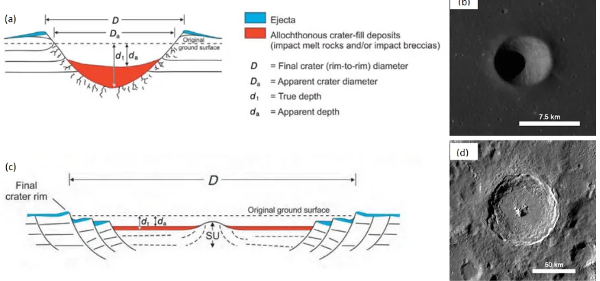
1.1 Cross-sectional diagrams of both a simple (a) and complex (c) crater
(Osinski & Pierazzo, 2012). (b) shows a WAC mosaic image of Sarabhai
crater, a 8 km diameter simple impact crater in Mare Serenitatis. Below
(d) is Tycho, an 86 km diameter complex crater in the southern lunar
highlands. Note the presence of the structural central uplift (SU) and
terraced walls. . . 3
1.2 Plots of depth-to-diameter ratio of detected Martian craters as a function
of southern latitude, from (Stepinski, Mendenhall, & Bue, 2009). Grey
dots are ‘shallow’ craters, black are ‘deep’, and the larger circles represent
binned measurements. A steep drop-off in d/D is measured around 38◦ S
in all three areas; this is potentially correlated to a significant increase in
the presence of ground ice. . . 5
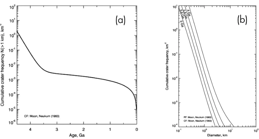
1.3 (a) The lunar chronology function. (b) A sample size-frequency
distribution (SFD), showing isochrons for 3.0, 3.6, 3.8 and 4.0 Ga. These
plots were generated using CraterstatsII (Michael & Neukum, 2010). . . . 6
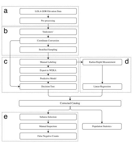
lines collect related steps. a: data collection and preprocessing b: crater
detection and categorization c: machine learning and training set
generation d: measurement accuracy and systematic error e: detection
efficiency assessment . . . 19
2.2 Global lunar map in simple cylindrical projection. This map is a
combination of 3 optical mosaics consisting of imagery from the Wide
Angle Camera (WAC), in addition to colour elevation information from
the LOLA instrument (red is high elevation, blue is low). Each study
area, demarcated by the white boxes, is roughly 90,000 km2. . . 20
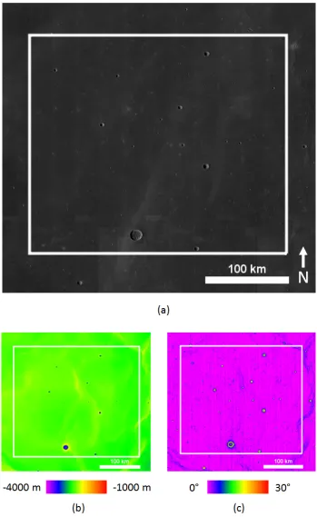
2.3 (a) Optical WAC mosaic of the Mare Serenitatis study area, at 100
m/pix. (b) Colourized elevation from the LOLA instrument. (c) Slope
map, derived from the LOLA DTM. . . 22
2.4 (a) Optical WAC mosaic of the Orientale ejecta study area, at 100
m/pix. (b) Colourized elevation from the LOLA instrument. (c) Slope
map, derived from the LOLA DTM. . . 24
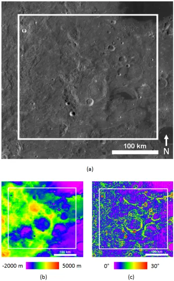
2.5 (a) Optical WAC mosaic of the Southern highlands study area, at 100
m/pix. (b) Colourized elevation from the LOLA instrument. (c) Slope
map, derived from the LOLA DTM. . . 26
system. Using an input DTM, the image is blurred at different spatial
scales to separate nested depressions. Craters detected in each blurred
landscape are recombined for the final catalog. Not all blurred
landscapes are shown for the sake of simplicity. . . 31
2.7 Graphic representation of the training set generation process. Each basin
that was selected via sampling is hand labeled as a crater or non-crater by
overlaying the rim on both optical and elevation data in JMARS. . . 35
2.8 Decision tree built using the training set for the Southern Highlands study
area. This tree was generated using the J48 machine learning algorithm in
the WEKA software suite. Nodes are ellipses and leaves are rectangles. At
each node, the numbers in parenthesis represent the number of instances
reaching the leaf (green) /the number of misclassified instances at the leaf
(red). . . 38
2.9 Automated crater detection results for study areas 1-3 (L to R,
respectively). These maps show the complete crater catalogues after
pruning. Background imagery is a 100 m/pix WAC mosaic. . . 43
2.10 Post-pruning cumulative distribution function (CDF) for the three study
areas. . . 43
2.11 Small basins detected by Cratermatic. Note the vertically-linear
arrangement. These basins do not survive the crater discrimination
process, and are artefacts caused by the laser altimetry data type. . . 45
100 km. Green crater profiles represent true positive detections, yellow
are false positive, and red are false negative with D >600 m. . . 51
2.13 The three performance metrics DET (solid line), Q (dashed line) and B
(dotted line) as a function of crater radius in pixels. Mare Serenitatis is
represented in blue, Orientale in green, and the Southern highlands in red. 52
2.14 A false positive detection in Mare Serenitatis. (a) The Cratermatic
detection result (b) The feature, as seen in LROC NAC optical imagery
(c) The feature as seen in the raw LOLA DTM. . . 53
2.15 Histogram of the depth-to-diameter ratio for all pruned craters withD >1
km. . . 54
2.16 SFD for each study area, plotted using CraterstatsII (Michael & Neukum,
2010). Three isochrons representing crater populations for 3.4, 3.8 and
4.0 Ga old surfaces are plotted as solid grey lines. Crater frequencies are
binned in pseudo-logarithmic fashion (18 bins per decade). . . 55
Hynek, 2012b). All imagery is THEMIS Day IR. (a) A 23 km diameter
crater in the pristine class (4), located at 16.50◦N 11.49◦E. Note the sharp
rim, central pit, and pristine ejecta. (b) A 44 km diameter class 3 crater
located at 14.79◦N 9.63◦E. This crater shows some infilling, as well as
subsequent cratering on the ejecta blanket. (c) A 65 km diameter class 2
crater, located at 15.27◦S 9.79◦E. This crater shows substantial infilling,
as well as minimal expression of the rim and ejecta. (d) A 38 km diameter
class 1 crater, centred at 39.33◦S 15.25◦E. This crater has no raised rim,
and is heavily infilled. Ejecta texture is no longer visible. . . 77
3.2 An example of a crater from each interior morphology class, from (Robbins
& Hynek, 2012b). All imagery is THEMIS Day IR. (a) A 30 km diameter
crater exhibiting a central peak (CpxCPk), or localized topographic high
near the crater center. This crater is located at 26.31◦N 28.12◦E. (b)
A 38 km diameter central pit (CpxCPt) located at 14.68◦N 20.67◦E. (c)
A 28 km diameter crater with a flat floor morphology (CpxFF), located
at 8.81◦N 35.82◦E. (d) A 19 km diameter summit pit crater (CpxSuPt),
centred at 15.24◦N 16.45◦E. The summit pit, located at the crater center,
is differentiated from a central pit by the raised topography on which the
pit is situated. . . 78
at 15.4◦N, 3.7◦E. The green line denotes the direction of the extracted
profile in (b). (b) A scaled plot of the crater profile (black), alongside
three Chebyshev profile approximations. As the order of approximation
increases from M = 4 (red) to M = 32 (blue), the approximation error is
reduced. . . 83
3.4 A general diagram of how crater profile reconstruction relates to basis
functions and coefficients. Each basis function, shown on the left as
Tn(x), has a weighted contribution to the final profile that is related to
its coefficientCn(x). . . 84
3.5 Flowchart of the major steps for this project. . . 86
3.6 Global map of Mars in simple cylindrical projection. Visualized data is
MOLA Colourized Elevation. The study area is outlined by the white box. 88
3.7 Profile extraction and approximation process. (a) Crater is identified by
catalogue values for location and radius. (b) Line of greatest slope
(white/red dashed line) through crater center and length 4·Rcrater is
identified. (c) Topographic profile is extracted, with domain scaled to
[-1,1]. (d) Profile is approximated using Chebyshev polynomial
expansion. (e) Chebyshev coefficients are retrieved from the expansion. . 91
3.8 (a) A THEMIS image of a 14 km crater, catalogued as degradation class
3 but misclassified as class 1. (b) The 2-D profile and Chebyshev
reconstruction of the crater, showing a significant pre-impact slope. . . . 102
3 but misclassified as class 1. This crater is in the ejecta blanket of
Cerulli, a 130 km diameter crater to the north. (b) The 2-D profile and
Chebyshev reconstruction of the crater, showing a good reconstruction
despite misclassification. . . 102
3.10 (a) A THEMIS image of a 20 km diameter crater with a central pit,
located at 30.35◦N, 18.60◦E. The pit is visible in the crater center. (b)
The extracted topographic profile (blue line) and reconstructed
Chebyshev approximation (red dashed line). The central pit, noticeable
as the dip in the elevation profile, is distinctly missing from the
approximation. . . 104
3.11 (a) A THEMIS image of a 21 km diameter crater with a central peak,
located at 22.09◦N, 8.71◦E. The peak is visible in the crater center. (b)
The extracted topographic profile (blue line) and reconstructed Chebyshev
approximation (red dashed line). This crater, listed in the source catalogue
as unclassified (CpxUnc), exhibits a strong central uplift signature with a
small summit pit when viewed as a 2D profile. . . 105
3.12 (a) A THEMIS image of a heavily degraded 42 km crater located at
18.95◦N, 20.81◦E, catalogued as CpxFF (flat floor) but given an
‘unclassified’ designation by the model. The south-west rim of the crater
is superposed by a very pristine 11 km crater. (b) The 2-D profile and
Chebyshev reconstruction of the crater, showing a rough interior
topography. . . 106
2.1 Details for the 3 selected study areas. . . 21
2.2 The six size-based crater classes. Craters are separated into classes based
on their diametric size to perform a stratified sampling and build the
training sets. . . 33
2.3 Numerical crater detection results for each study area. . . 44
2.4 Linear regression results for radius and depth in all three study areas.
These fits were used to correct the values of the pruned crater catalogue.
The true values are measured manually and are used to corrected the
detected values. . . 46
2.5 Detailed accuracy statistics for ‘crater’ class, for each study area. . . 49
2.6 Detailed accuracy statistics for ‘non-crater’ class, for each study area. . . 50
2.7 Comparison of performance metrics with other published values. * The
values listed for the three study areas here are for craters with D≥4 km. 57
3.1 Crater degradation classification criteria from (Robbins & Hynek, 2012a). 76
3.2 List of Chebyshev coefficients and coefficient combinations, with their
interpreted topographical indications (Mahanti, Robinson, Humm, &
Stopar, 2014). . . 85
number of instances listed is from the original catalogue. . . 96
3.4 Confusion matrix for the degradation class assessment. . . 96
3.5 Interior morphology assignment results for the classification model. The
number of instances listed is from the original catalogue. CpxUnc is
unclassified, CpxCpk is central peak, CpxCpt is central pit, CpxFF is
flat-floored, and CpxSuPt is summit pit. . . 97
3.6 Confusion matrix for the interior morphology class assessment. . . 97
3.7 Degradation classification results for class combinations. The original 4
class results are listed, as well as the 3 class (degraded, moderately
preserved/degraded, well preserved) and 2 class combination (degraded,
preserved). . . 101
Appendix A MATLAB Algorithms and Decision Trees . . . 120
Appendix B Crater Degradation Classification . . . 123
Nomenclature
ASCII American Standard Code for Information Interchange CDA Crater Detection Algorithm
CDF Cumulative Distribution Function
Cn n-th Chebyshev Polynomial Coefficient
CSV Comma Separated Values
d/D Depth-to-Diameter
DTM Digital Terrain Model
FN False Negative
FP False Positive
GDR Gridded Data Record
GLD Global Lunar DTM
JMARS Java Mission-planning and Analysis for Remote Sensing
lat Latitude
LOLA Lunar Orbiter Laser Altimeter
lon Longitude
LRO Lunar Reconnaissance Orbiter
LROC Lunar Reconnaissance Orbiter Camera
MGS Mars Global Surveyor
MOLA Mars Orbiter Laser Altimeter
NAC Narrow Angle Camera
PDS Planetary Data System
pix pixel
SFD Size-Frequency Distribution
THEMIS Thermal Emission Imaging System
TP True Positive
WAC Wide Angle Camera
WEKA Waikato Environment for Knowledge Analysis
Introduction
1.1
Impact Cratering
Impact craters are basin-shaped features on a surface formed by a collision of an
asteroid, comet or meteoroid on that surface. The structures are ubiquitous throughout
the solar system, and are studied by a large community of planetary and earth
scientists. Impact craters (hereafter just ‘craters’) exhibit different expressions and
properties that depend on the pre-impact surface conditions, subsurface composition,
and parameters of the impact event such as energy and impact angle. Additionally,
they can be altered over time by surface processes which vary depending on celestial
body. Craters can be divided into main groups: simple and complex. These two groups
are separated by size; above a certain threshold, the crater transitions to a complex
shape with a central peak. This transition size for a given body is related to its
gravitational acceleration (Melosh, 2011). The anatomy of both a simple and complex
crater are shown in Figure 1.1.
Simple craters are bowl-shaped, with an uplifted rim that can be altered by
weathering or other modifying processes. The floor of the crater contains a mix of
breccia (broken fragments of target material held together in a matrix) and possibly
impact melt (target rock that was melted from the extreme heat of impact). Beyond
the rim of the crater, debris known as ejecta is deposited on top of the surrounding
terrain, with the thickness of the ejecta being inversely related to radial distance from
the rim (McGetchin, Settle, & Head III, 1973). This ejecta, while relatively thin for
smaller craters, can play a significant role in altering the landscape as the impact and
thus amount of excavated material becomes larger. Significantly large enough impacts
are known to form impact basins (hereafter referred to as ‘impact basins’ in full to
identify them from regular topographic depressions). These structures, such as the one
that formed the Orientale Basin, have diameters on the order of hundreds to thousands
of km, and often form concentric ring systems. Impact basins have an age-resetting
effect on the terrain surrounding them. Proximal craters will be entirely covered, while
craters that are further out will be significantly in-filled so as to fundamentally change
their expression. Craters which have been in-filled by either ejecta or lava, but still have
a visible raised rim, are known as ghost craters. Ghost craters can affect crater counts
and throw off age estimates.
The topographic expression of simple craters can be described to a lower degree as a
local region of concavity. The morphology changes for craters that have a diameter
Figure 1.1: Cross-sectional diagrams of both a simple (a) and complex (c) crater (Osinski & Pierazzo, 2012). (b) shows a WAC mosaic image of Sarabhai crater, a 8 km diameter simple impact crater in Mare Serenitatis. Below (d) is Tycho, an 86 km diameter complex crater in the southern lunar highlands. Note the presence of the structural central uplift (SU) and terraced walls.
km for Mars and between 3 km and 5 km on Earth (Melosh & Ivanov, 1999). Complex
craters, which have diameters above the transition size, are structurally different from
their simple counterparts. In addition to the raised rim and ejecta features, complex
craters exhibit a significant central peak, or local topographic high at the center of the
crater. Additionally, complex craters can have terraced walls from collapse, which cause
the rim to take on a more polygonal shape over time as the crater is modified.
Quantities such as depth, circularity and continuity of the rim crest that describe the
shape of a crater can be affected over time by various modifying processes. This has
consequences for the automatic detection and measurement of these craters, as the
The spatial and morphometric analysis of impact craters has proven over decades to
be a useful tool for answering a variety of questions in planetary science. Early work
established the use of impact crater studies in providing chronological information
about the lunar surface, laying the foundation for a stratigraphic history of the Moon
(Opik, 1960; Shoemaker, Hackman, & Eggleton, 1963; Hartmann, 1965). Additionally,
impact crater populations have helped constrain models of impactor populations
(Neukum, K¨onig, & Fechtig, 1975). Modern applications of impact crater morphometry
have revealed information about crater formation processes (Xiao, Zeng, & Komatsu,
2014), as well as surface (Bart, 2014) and subsurface (Pathare, Paige, & Turtle, 2005)
crustal compositions. An example of using crater morphometry to identify the presence
of ice is shown in Figure 1.2. The study and detection of impact craters is also relevant
to the field of space exploration and has been used to investigate autonomous
spacecraft landing systems (Leroy, Medioni, Johnson, & Matthies, 2001; Johnson,
Huertas, Werner, & Montgomery, 2008).
1.2
Crater Chronology
As mentioned previously, impact craters have been used as a tool to deduce the relative
ages of surface units since the 1960’s (Bland, 2003). Prior to the Apollo landings of the
late 1960’s and early 1970’s, it was highly desirable to form a lunar geologic record so
as to inform the landings and subsequent sample collection. Early work in lunar
chronology employed crater counting as a means to deduce relative ages. Resting on the
Figure 1.2: Plots of depth-to-diameter ratio of detected Martian craters as a function of southern latitude, from (Stepinski et al., 2009). Grey dots are ‘shallow’ craters, black are ‘deep’, and the larger circles represent binned measurements. A steep drop-off in d/D is measured around 38◦ S in all three areas; this is potentially correlated to a significant increase in the presence of ground ice.
technique involves counting the densities of craters of varying size that are found on the
unit. By modelling and estimating the production rate, or rate at which craters of a
given size are formed on the surface, it is possible to extract the age. It is then possible
to calibrate these to absolute ages when compared against radiometrically dated
samples from the Apollo missions. While this calibration can only be performed for
bodies where physical samples have been obtained, more recent work has extended the
crater production function from the Moon to other bodies such as Mars by examining
impact rate and scaling law differences for the separate bodies. The crater density
above a certain diameter has historically been expressed by a power law relationship, of
the form
Ncum(D) = cDb (1.1)
value known as the size index, and c is a constant (Basaltic Volcanism Study Project,
1981). In (Neukum, 1983), the surface density of craters was related to the surface age
by the chronology function
N(D >1) = 5.44·10−14(e6.93T −1) + 8.38·10−4T (1.2)
whereN(D >1) is the number of craters with a diameter larger than 1 km normalized to
the counting area in sq. km, and T is the age of the surface in billions of years (Ga). For
lunar surface calculations using the above equation and an automated crater detection
system, it is imperative to understand the system’s responsiveness for craters above 1
km as this will have an effect on the calculated age. The chronology function is shown
in Figure 1.3.
Figure 1.3: (a) The lunar chronology function. (b) A sample size-frequency distribution (SFD), showing isochrons for 3.0, 3.6, 3.8 and 4.0 Ga. These plots were generated using CraterstatsII (Michael & Neukum, 2010).
a size-frequency distribution. A SFD is a graphic representation of the density of craters
contained within a certain diameter bin, against diameter in a log-log plot. Equation
1.1 shows that one should expect a power-law relationship on the graph, with slope b.
However, various modifying processes affect crater densities, causing a deviation from
the perfect power law relationship (Williams, Pathare, & Aharonson, 2014). This effect
is strongest in the small-D regime. In addition, SFDs can be used to plot isochrons, or
lines of constant age on a SFD. For a given surface unit, an older age will mean a higher
crater frequency for a given diameter bin. This will push older isochrons (or surface
populations) to the right on the SFD plot. Comparison of these isochrons against the
results of a crater count gives both an idea of the surface’s age, as well as any modifying
processes that cause the crater count to deviate from an ideal distribution.
1.3
Research Objectives
This thesis will examine the role of automated image processing methods for impact
crater analysis. In doing so, it seeks to address the following questions:
1. Does lunar surface terrain type variation affect the results of automated crater
detection?
2. What influences systematic measurement error using automated measurement
systems?
3. How can the results of automated crater detection and measurement be applied to
4. Can an objective crater degradation classifier be built using a polynomial profile
approximation method?
5. How can existing crater catalogues be used to improve automated crater
characterization methods?
6. Are automated methods alone currently sufficient for crater characterization?
The major research objectives are as follows:
1. To apply a topographic crater detection system to three distinct lunar surface
types; to compare the results against visual inspection of the surface to determine
detection efficiency as a function of crater size; to compare extracted radii and
depths against measured values to identify systematic measurement error; and to
build a crater chronology and bulk statistical description of the craters for each
unit type and compare them against previous results.
2. To build an automated, quantitative method for the degradation and interior
morphological classification of martian complex impact craters; to apply
polynomial approximation methods to the craters’ topographic profiles; to use the
approximations as discriminators in a classification model; and to identify the
classification accuracy of such an approach.
1.4
Thesis Organization
This thesis is presented in integrated article format. It contains two two papers that
Chapter 1 introduces some background on impact craters and provides research topic
context. Additionally, it outlines the research objectives. Chapters 2 and 3 are two
individual but related studies. Chapter 2 presents a study on the effect of lunar terrain
type variation on automated crater detection and measurement. This work was
presented at the 47th Lunar and Planetary Science Conference in Houston, Texas.
Chapter 3 describes the development of an automated crater degradation state classifier
using polynomial profile approximations. Chapter 4 concludes the thesis, describing the
primary findings of the work and discussing future applications of automated digital
Bart, G. D. (2014). The quantitative relationship between small impact crater
morphology and regolith depth. Icarus, 235, 130–135.
doi: 10.1016/j.icarus.2014.03.020
Basaltic Volcanism Study Project. (1981). Basaltic Volcanism on the Terrestrial Planets.
New York: Pergamon Press, Inc.
Bland, P. (2003). Crater counting. Astronomy and Geophysics, 44(4), 4.21–4.21.
doi: 10.1046/j.1468-4004.2003.44421.x
Hartmann, W. K. (1965). Terrestrial and Lunar Flux of Large Meteorites in the Last
Two Billion Years. Icarus, 4(2), 157–165.
doi: 10.1016/0019-1035(65)90057-6
Johnson, A. E., Huertas, A., Werner, R. A., & Montgomery, J. F. (2008). Analysis
of On-Board Hazard Detection and Avoidance for Safe Lunar Landing. Aerospace
Conference, 2008 IEEE, 1–9.
doi: 10.1109/AERO.2008.4526301
Leroy, B., Medioni, G., Johnson, E., & Matthies, L. (2001). Crater detection for
autonomous landing on asteroids. Image and Vision Computing,19(11), 787–792.
doi: 10.1016/S0262-8856(00)00111-6
McGetchin, T. R., Settle, M., & Head III, J. W. (1973). Radial thickness variation in
impact crater ejecta: implications for lunar basin deposits. Earth and Planetary
Science Letters,20(2), 226–236. doi: 10.1016/0012-821X(73)90162-3
Melosh, H. J. (2011). Planetary Surface Processes (1st ed.). Cambridge University Press.
doi: 10.1017/CBO9780511977848
Melosh, H. J., & Ivanov, B. A. (1999). Impact Crater Collapse. Annual Review of Earth
and Planetary Sciences, 27(1), 385–415.
doi: 10.1146/annurev.earth.27.1.385
Michael, G., & Neukum, G. (2010). Planetary surface dating from crater
size-frequency distribution measurements: Partial resurfacing events and statistical age
uncertainty. Earth and Planetary Science Letters, 294(3-4), 223–229.
doi: 10.1016/j.epsl.2009.12.041
Neukum, G. (1983). Meteoritenbombardement und Datierung Planetarer Oberflaechen
. Habilitation Dissertation for Faculty Membership, Univ. of Munich, 1–186.
Neukum, G., K¨onig, B., & Fechtig, H. (1975). Cratering in the earth-moon system:
Consequences for age determination by crater counting. Proc. Lunar Planet. Sci.
Conf. 6th, 2597–2620.
Opik, E. (1960). The Lunar Surface as an Impact Counter. Oxford Journal, 120(5),
404–411.
Osinski, G. R., & Pierazzo, E. (2012). Impact Cratering: Processes and Products
(G. R. Osinski & E. Pierazzo, Eds.). Chichester, UK: John Wiley & Sons, Ltd.
within the martian south polar layered deposits. Icarus,174(2), 396–418.
doi: 10.1016/j.icarus.2004.10.031
Shoemaker, E., Hackman, R., & Eggleton, R. (1963). Interplanetary Correlation of
Geologic Time. Advances in the Astronautical Sciences, 8, 70–89.
Stepinski, T. F., Mendenhall, M. P., & Bue, B. D. (2009). Machine cataloging of impact
craters on Mars. Icarus,203(1), 77–87.
doi: 10.1016/j.icarus.2009.04.026
Williams, J. P., Pathare, A. V., & Aharonson, O. (2014). The production of small
primary craters on Mars and the Moon. Icarus,235, 23–36.
doi: 10.1016/j.icarus.2014.03.011
Xiao, Z., Zeng, Z., & Komatsu, G. (2014). A global inventory of central pit craters on
the Moon: Distribution, morphology, and geometry. Icarus, 227, 195–201.
The Effect of Lunar Terrain Type
Variation on the Results of
Automated Crater Detection
2.1
Introduction
2.1.1
Automatic Crater Detection
Traditionally, impact craters were catalogued and measured manually, with visual
inspection of stereoscopic images or utilizing shadow sizes and viewing geometry. This
technique was hindered by low resolution imagery and inherent inconsistencies between
experts. Around the year 2000, researchers began searching for a fully automated
impact crater detection algorithm (CDA). An ideal CDA would be robust under
varying surface conditions, independent of lighting conditions or viewing geometry
inherent to the data, and scale invariant. As planetary surface data became digitally
available, the fields of image processing and computer science lent their developments
to the task of crater detection. Early CDAs (Jahn, 1994; Honda et al., 2000; Alekseev,
Pyatkin, & Salov, 1993) worked on photographic imagery, using edge detection and the
Hough transform circular feature extraction tools in imagery. More complex systems
(Kim et al., 2005; Sawabe, Matsunaga, & Rokugawa, 2006) included machine learning
methods and image pipelines to improve their detection capabilities.
Newer systems have sought to improve the state of CDAs by using topographic data,
primarily in the form of digital terrain models (DTMs). There are two primary arguments
to be made for using elevation data: 1) impact craters manifest with a particularly
strong topographic signature, and such a signature can be uniquely detected, and 2)
this signature is independent of viewing conditions such as lighting or geometry. The
Mars Orbiter Laser Altimeter (MOLA) instrument aboard Mars Global Surveyor (MGS)
helped advance progress in the area of crater detection. Initially, 2-D line tracks of
elevation were used alongside edge detection schemes to assist in crater identification
(Kim, Muller, & Morley, 2000). Later systems (Michael, 2003; Kim, Muller, & Morley,
2004; Bue & Stepinski, 2007) were able to apply advanced image processing techniques
to DTMs, with varying results in different study areas. One particular system known
as the AutoCrat system (Stepinski, Mendenhall, & Bue, 2009) used a novel mixture of
image processing and machine learning to detect craters on the martian surface, using
a MOLA-derived DTM. The AutoCrat system combines topographic image processing
employed in this project, will be described in greater detail in the following chapters.
2.1.2
CDA Accuracy
The lack of a perfectly accurate and scale-invariant CDA has meant that each detection
system contains some error in its detection efficiency, measurement, or both. Whether
using a CDA for generating an age estimate or collecting bulk crater morphometric
characteristics, these errors are likely to affect the scientific validity of the end product in
some way. Many CDAs are compared directly against a set of craters that are
manually-labelled by a human expert, often in the form of a catalogue. This process provides a
good first order understanding of the CDA’s inaccuracy. However, it is also important
to control some of the testing variables in a manner to more broadly understand the
system’s accuracy and response to change. Some of these variables include geomorphic
unit, crater size regime, and elevation data type. While there have been many published
CDAs, achieving varied levels of success, there isn’t yet a consistent framework for the
objective evaluation of these systems (Salamuni´ccar & Lonˇcari´c, 2008). Different authors
use different test areas, catalogues of ground-truthed craters, and different statistical
measures of accuracy. A previous study using elevation data for Mars briefly examined
the effect of automated crater detection on four different geomorphic units: volcanic, sea
(planitia), and two plateaus (planum) (Yin, Xu, Li, & Liu, 2013). Significant differences
2.1.3
Purpose
This paper presents an in-depth evaluation of the AutoCrat system, using
high-resolution elevation data for the lunar surface unavailable at the time the system
was originally designed. As identified in previous work, there is a need for the objective
evaluation and cross-comparison of CDAs (Salamuni´ccar & Lonˇcari´c, 2008). As the
AutoCrat system is a particularly pure example of a topographic CDA (using only the
topography, and no optical data or template matching), it is investigated using three
different ‘characteristic’ lunar terrains to determine the robustness with varying surface
type. Detection results can be compared against true images of the terrain to identify
the strengths and weaknesses of a topographic approach to crater detection. As an
additional objective, the population statistics of detected craters is investigated. By
examining these statistics and their related accuracies, one can assess the validity of
using the results for surface unit dating, or extraction of bulk morphometric properties.
For the sake of comparison, this work does not involve a re-parametrization of the
original system, nor does it change the machine learning algorithm used in
discrimination. This will be further explained in Section 2.2.1.
We begin by explaining an overview of the project methodology. This includes a
thorough discussion of the data type chosen, as well as the motivation for choice of
study areas. Both the crater detection and discrimination systems will be described,
in addition to the statistical methods chosen for assessment of the results. Finally, the
and compared with similar systems previously used in the literature. Closing with a
discussion, we present themes on the dependency of terrain morphology on automated
crater detection.
2.2
Methods
2.2.1
Overview
This study applied a set of processing steps on three digital elevation models
representing topographically distinct regions of the lunar surface. These steps are
grouped and identified with bold letters in the flowchart shown in Figure 2.1. For the
sake of consistency, the processing and statistical analysis was replicated in all three
areas. One of the three study areas used a DTM with a different resolution; this is
further discussed in Section 2.2.2. The project is composed of five major steps: data
collection, initial processing, machine learning discrimination, measurement accuracy,
and detection efficiency assessment. Generally, each equal-area region was extracted
from a larger DTM and preprocessed (box a). Next, a basin detection routine is run on
the DTM, generating the preliminary crater candidates (box b). Using a discrimination
algorithm generated by a machine learning method (c), the subset of impact craters is
extracted from that set. Finally, corrections to the crater measurements are made (box
d) and accuracy assessment is undertaken on the members of the final catalogue (box
The statistical analysis of the crater detection output is compared for the three
study areas. Results such as detection efficiency and measurement accuracy are the
primary focus. Additionally, we can comment on the viability of the results for use in
both age estimation and population statistics. A combination of stratified sampling and
linear regression are used in performing these assessments.
The AutoCrat system is a two-stage crater detection and discrimination system,
using image processing operations on digital images representing elevation profiles of a
landscape. This system approaches automated crater detection from a different angle
than many other CDAs. In place of complicated systems that require constant
re-parametrization for different data sets and on different spatial scales, the AutoCrat
uses an impact crater’s unique topographic signature as the basis of its modus
operandi. In principle, a crater’s topographic signature is independent of lighting
conditions, viewing geometry or other instrument variation. Using some DTM image
processing techniques, the AutoCrat system can find even nested depressions while
operating under scale-invariance.
The primary crater finding algorithm, after operating on a DTM dataset, produces
a catalog of crater candidate positions, depths and radii, and some mathematical shape
descriptors. By seeking all nearly-circular depressions, the first portion of the system
seeks completeness through performing an exhaustive search. This should minimize the
number of false negative detections (missing craters). A second machine learning stage
part provides accuracy by refining the preliminary catalogue of depressions, or
minimization of false positives. A summarized description of these two steps will be
given in the following subsections. For a more detailed description of the algorithm and
its nuances, please consult (Stepinski et al., 2009). The two parts of the AutoCrat
system are shown in boxes b and c in Figure 2.1.
2.2.2
Study Areas and Data
Figure 2.2: Global lunar map in simple cylindrical projection. This map is a combination of 3 optical mosaics consisting of imagery from the Wide Angle Camera (WAC), in addition to colour elevation information from the LOLA instrument (red is high elevation, blue is low). Each study area, demarcated by the white boxes, is roughly 90,000 km2.
In examining the robustness of a CDA, broad-scale terrain morphology has been
identified as a source of inconsistency in crater detection results (Li, Ling, Zhang, &
Wu, 2015). As such, it is necessary to apply a CDA to different types of terrain for a
more complete understanding of its performance. Additionally, for CDAs that also
measurement response and variation with changing terrain. On the Moon, this includes
the two major terrain types that comprise the lunar surface dichotomy: the light-toned,
older, more heavily cratered highlands and the darker, younger maria. Additionally,
there are the ejecta blankets of large basins, which deposit enormous amounts of
material atop the surrounding terrain. These three terrain types collectively
characterize much of the Moon’s surface, while remaining distinct from each other
individually. They can be thought of as a ‘basis set’ of terrain morphologies. By
understanding the response of a CDA to these three units collectively, it can be
employed on a majority of the lunar surface in a predictable fashion.
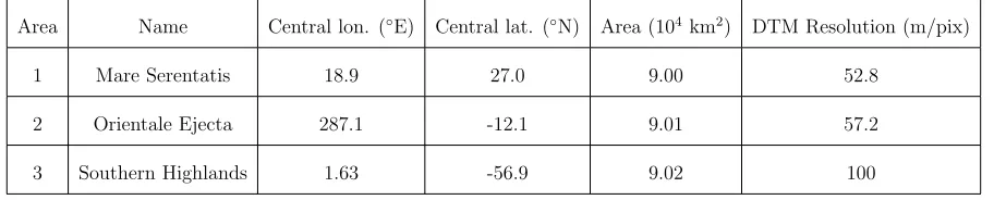
Table 2.1: Details for the 3 selected study areas.
Area Name Central lon. (◦E) Central lat. (◦N) Area (104km2) DTM Resolution (m/pix)
1 Mare Serentatis 18.9 27.0 9.00 52.8
2 Orientale Ejecta 287.1 -12.1 9.01 57.2
Study Area 1 - Mare Serenitatis
Mare Serenitatis is a∼675 km diameter impact basin on the lunar nearside. It contains
a dark-toned surface unit, which together with other similar units on the moon are
collectively called ‘maria’. The southeastern edge of Mare Serenitatis was visited by
humans during the Apollo 17 mission in 1972. The maria, covering a total of about
17% of the lunar surface, are large basaltic plains that were emplaced by previous
volcanic activity (Head III & Wilson, 1992). Typically, mare are relatively flat on large
scales, with a more sparsely cratered surface. Previous mapping of Mare Serenitatis has
subdivided the mare into many regions with varying ages. Surface unit dating and
regional albedo differences imply that volcanism within the interior of the basin took
place for hundreds of million years after the formation of the basin, leading to surface
ages of roughly 3.4 - 3.8 Ga (Hiesinger, Jaumann, Neukum, & Head III, 2000).
In addition to craters, the surface of the mare can exhibit wrinkle ridges and
differences in tone. Few craters on the scale of tens of kilometres can be seen, as visible
in the optical image from Figure 2.3. As the spatial scale under study is made more
fine, both crater densities and local topographic variation increase. From a crater
detection perspective, this unit type should be simplest. This is because of the flat
pre-impact terrain and sparse cratering. In the chosen study area comprising of about
one quarter of the total area of Mare Serenitatis (Whitford-Stark, 1982), there are no
complex craters. Based on a study analysing the pulverization and overturning of the
mare regolith, the mare surface should have saturation of craters up to roughly
D = 200 m (Hartmann & Gaskell, 1997). This process is what gives the mare its
Study Area 2 - Orientale Ejecta
The Orientale Basin is a multi-ring impact structure on the western limb of the lunar
nearside. A well-preserved structure, it is thought to have formed at the end of the Late
Heavy Bombardment around 3.8 Ga ago (Spudis, Martin, & Kramer, 2014), a period of
intense cratering in the early solar system. Measuring around 930 km in diameter, the
impact basin’s formation into underlying highland material affected much of the
surrounding terrain, and lunar surface on the whole. The emplacement of ejecta on the
surrounding terrain caused a proximal age resetting by modifying the prebasin
population up to a distance of 2 basin radii from the center (Head III et al., 2010).
Additionally, Orientale can be used to distinguish the presence of two populations of
impactors, with the transition between the two occurring near the time the Orientale
Basin formed.
The study area for this project consists of the ejecta to the east and north of Orientale,
just outside the Cordillera Mountain ring. This is within the area of age resetting, but
since the study area extends significantly far in the radial direction from the center,
there is expected to be some local variation in the terrain as the ejecta emplacement is
non-uniform. As evident in the slope map in Figure 2.4(c), this terrain is more complex
than the mare areas. Significant undulations caused by ejecta and the pre-basin terrain
mean greater variation in slope on coarse scales. This will be a significant challenge for
the CDA. Large craters that were on the pre-basin terrain may still present topographic
Study Area 3 - Southern Highlands
The lunar highlands are the oldest terrains on the Moon. Lighter in colour than their
mare counterparts, they are primarily composed of anorthosite, an intrusive igneous
rock (Pieters, 1986). At higher elevation than the mare, they consist of the southern
portions of the lunar nearside, and a significant percentage of the farside. The
highlands have dense associations of impact craters, even in some areas achieving
complete empirical saturation (Hiesinger et al., 2000) (the addition of any new crater is
guaranteed to erase a pre-existing crater of comparable diameter). A state of empirical
saturation is challenging for extracting surface ages from crater counts. This is because
as new craters are formed, the total crater density for a given size range is unchanged,
while the underlying crustal rock is obviously still getting older. Additionally, complex
craters are most abundant in the highlands, with varying states of degradation. Many
complex craters have been partially superposed by other craters, often eliminating
significant portions of the rim.
The highlands study area is on the lunar nearside, towards the south pole. This study
area poses a challenge for a CDA, as it has the highest requirement of scale-invariance.
The presence of craters at a wide variety of diameters requires the system to be responsive
to both small simple craters, as well as large complex craters. Additionally, the age of
the surface indicates a larger array of crater degradation states - ranging from relatively
Source Data
The data chosen for this study are reduced and gridded DTMs generated by the LOLA
instrument. These DTMs are freely available from the LOLA PDS Data Node at
imbrium.mit.edu. LOLA, a laser altimeter and passive infrared radiometer on board the Lunar Reconnaissance Orbiter (LRO), is a time-of-flight laser altimeter which fires
pulses of 5 infrared lasers onto the lunar surface at a frequency of 28 Hz (Neumann,
2011). By using 5 spots to sample the ground, the instrument can collect both
along-track slope and across-track slope, in addition to measuring the
spacecraft-to-ground distance (which can be used to calculate absolute elevation). Since
the Moon does not have the notion of ‘sea level’, all elevations are measured relative to
the selenoid, or a perfect sphere of radius 1,737 km.
As the spacecraft travels, measurements from the 5 spots are collected and used to
construct a 2-D line of elevation along the spacecraft’s ground track. Over time, these
tracks have collected over the lunar surface. Due to LRO’s arrangement in a polar
orbit, the tracks are densest at the poles, and spaced most widely at the equator. From
these tracks, a minimum-curvature interpolation is performed to fill in the space
between tracks, providing a complete 3-D elevation model for the lunar surface. It is
important to note the mathematical method of generating the 3D surface, as this will
have an effect on the precision of the crater detection results. For any given pixel in the
DTM that does not contain a direct LOLA elevation measurement, a mathematical rule
derivative, and minimizes overall curvature. While this provides a smooth surface, it
makes assumptions about the surface that may not necessarily be true. In addition,
craters whose diameters are significantly smaller than the cross-track width may be
missed entirely.
To start, the appropriate DTM is selected from the repository. This project uses
gridded data record (GDR) DTMs, which have undergone higher-level processing which
includes binning, resampling and map projection. First, we located the appropriate
parent DTMs which contain the study areas. For the equatorial study areas, DTMs in
cylindrical map projection that span 45◦ of latitude and 90◦ of longitude were
downloaded. The study area in the southern highlands is found in a south polar
stereographic DTM. Next, the region of interest containing the study area was cropped
out with a mask in ArcGIS. The digital values in the raster were then converted to
elevations with respect to the selenoid by using a bulk raster calculation. Finally, the
DTM is exported as an ASCII text file, which allows it to be read by the Cratermatic
software. The DTM is now ready for crater detection.
For the sake of comparison with previous studies using DTMs of the martian surface
generated in a similar fashion (from the MOLA instrument), only LOLA data were chosen
for this study. Future work in automated crater detection can be expanded to DTMs
generated by other means and instruments. Further discussion of the consequences of
2.2.3
Crater Detection
This section details the process of identifying the crater candidates from a topographic
landscape. Beginning with a DTM covering a region of interest, a series of image
processing tasks are used to extract and compile the basins that form the initial list of
candidates.
Crater Detection - findcraters
The first stage of the AutoCrat system uses a topographic basin finding routine called
findcraters, which is within the Cratermatic topography analysis toolkit. This routine (box b in Figure 2.1) performs a series of image processing operations on a
topography dataset whose pixel values represent the elevation for that pixel; either
directly sampled from a LOLA track or via interpolation. Typically, identifying isolated
basins in a topographic landscape can be performed with the use of a watershed
algorithm (Meyer & Beucher, 1990), which segments the image into catchment basins.
This approach is unsuccessful in the case of nested basins, since the watershed
algorithm will simply combine the two into a single depression. The Cratermatic
system uses an image convolution to address this issue. Shown in Figure 2.6 is the
processing for a small sample region of the lunar surface.
The first step in crater detection is to apply an image convolution called a
C-transform. This transform is similar to a Gaussian blur, and acts to smooth the
smooths the landscape emphasizing depressions on the order of size λ. This helps to
identify nested depressions by ignoring depressions that are significantly larger or
smaller. After finding an anchor pixel around which all points are concave up, the
algorithm incorporates other pixels belonging to the crater region, stopping after a
slope threshold. The centroid is identified as the center-of-mass of the crater (as the
profile can be non-circular), and a polar function is used to represent the rim shape. A
Fourier expansion is used to build the polar function. Coefficients derived from the
Fourier expansion are used to describe the shape; a perfect circle would have all but the
first coefficients equal to zero. Therefore we can use the coefficients to describe
deviations from a perfect circle. Two particularly useful quantities derived from the
coefficients are m2, which describes the elongation of the crater shape, and m3, which
describes its ‘lumpiness’.
When the preliminary crater catalogue is produced, the crater locations are given in
the image space. For example, the catalogue will list one depression in the set as an
entry of the form {# ID, x, y, r, area, depth, m2, m3}. Coordinate conversions are then
performed on the catalogue to translate each centroid in x and y image space to a
planetocentric latitude and longitude, and to convert the radius to meters.
Stratified Sampling
The final step before categorizing the basins as crater or non-crater is to perform a
twofold and will be explained in greater detail in Section 2.2.5. Due to the uneven
detection distribution as a function of crater size, special care must be taken to sample
appropriately over the range of possible crater sizes in the landscape. To assess
measurement accuracies as a function of crater size, the craters need to be split up into
groups based on their diameters. We start by dividing craters into three major groups:
small craters (D<300 m), intermediate craters (300 m<D<4 km), and larger diameter
craters (D > 4km)(Melosh, 2011). From there, the intermediate class of craters is split
into three 1-kilometre sized groups between 1 and 4 km. The crater size categories are
shown below in Table 2.2.
Table 2.2: The six size-based crater classes. Craters are separated into classes based on their diametric size to perform a stratified sampling and build the training sets.
Class A B C D E F
Diameter D<300m 300m≤D<1km 1km≤D<2km 2km≤D<3km 3km≤D<4km D≥4km
The Cratermatic system works on iteratively larger radius scales, doubling the
radial pixel size for the Gaussian convolution each round. After reaching a size limit
which is dictated by the smaller dimension of the input image, the algorithm combines
all the detected basins from each scale and outputs a catalogue identifying the basin
location and quantities related to its size and shape. As mentioned previously, this is
(ideally) an exhaustive list ofdepressions, a subset of which will consist of only the true
craters. In the next section, we describe how machine learning can be used to extract
2.2.4
Crater Discrimination
The cadence of successful space missions over the past few decades has dramatically
increased the wealth of data that is available for many solar system objects. This large
amount of data has proven challenging to analyse in a time-efficient and thorough
manner. Not only is there simply too much to look at, but often the nature of the
analysis is quite complex and thus difficult for a human analyst to complete in
significant enough amounts over reasonable timescales. Advancements and techniques
in artificial intelligence and automated data analysis can be invaluable tools for such
tasks. Previously, machine learning has been applied to problems in planetary science
such as automated geologic mapping (Stepinski, Ghosh, & Vilalta, 2007) and surface
unit annotation (Ghosh, Stepinski, & Vilalta, 2010). In the context of automated crater
detection, machine learning can be used as a powerful tool for devising a set of rules to
discriminate craters from non-crater depressions.
Training Set Construction
In order to later instruct the machine learning algorithm how to discriminate crater
from non-crater, it is necessary to build training sets for each study area, consisting of
examples of both craters and non-craters. The training sets also provide an opportunity
to study the measurement accuracy of the system; this is elaborated on later in Section
2.2.5. For each study area, the list of crater candidates including their category
Figure 2.7: Graphic representation of the training set generation process. Each basin that was selected via sampling is hand labeled as a crater or non-crater by overlaying the rim on both optical and elevation data in JMARS.
are selected to begin constructing the training sets for each area. Each training set is
then exported to JMARS for visualization. Starting at the top of the list, each crater is
superimposed on optical data sets (primarily NAC image strips and WAC global
mosaics) and inspected. For the high-resolution NAC images, the incidence angle search
parameter is restricted to higher angles - typically between 45◦ and 80◦ to accentuate
topography. The candidate is then hand labelled as either crater or non-crater. It is
important to note here that individual craters of all types are labeled a crater,
including secondaries (craters formed by the impact of ejecta from another crater) and
ghost craters (craters heavily mantled by lava or other materials, leaving a faint rim).
As long as it represents one single crater, it is counted. Differentiating between crater
After each category has had its 20 craters labelled, additional craters from the
preliminary catalogue are added as necessary to provide equal numbers of true and false
craters. This is necessary as the basin-detection algorithm typically finds more
non-craters than craters (the degree to which this happens is a function of the
category), and thus balancing of the training set is necessary to improve the robustness
of the discrimination process. Exhaustive sampling of the larger crater categories (E
and F) occurred in study area 1, where large diameter craters aren’t as populous. After
manual labelling and any additions to the list, the training sets for study areas 1-3 had
143, 133 and 128 members respectively.
Decision Tree
As mentioned previously, machine learning in this context can generate a set of
discrimination rules to separate crater from non-crater. These rules, when structured
together, form the basis of a classification model. Fundamentally, this involves using a
set of quantified characteristics for which an impact crater will have some set of
identifying values. The pertinent values for this project are the quantities produced by
the Cratermatic algorithm: depth, diameter, depth-to-diameter ratio, and two
quantities derived from the Fourier coefficients described in Section 2.2.3 that are used
to describe the rim shape. The AutoCrat system uses a specific type of machine
learning algorithm, known as a decision tree classifier, to build the set of discriminatory
rules. This algorithm, called J48, is an open source Java implementation of the C4.5
algorithm (Quinlan, 1993). The algorithm is available through the Waikato
containing many tools for data mining (Hall et al., 2009).
In principle, the J48 algorithm works by finding attributes that most effectively split
the data into different classes. Given n examples, the training set can be expressed as a
set S = (s1, s2, ..., sn). Each sample si in the training set contains m attributes, in the
form (x1,i, x2,i, ..., xm,i) with one of the attributes being the class to which the sample
belongs. In this project, the set S is the training set with si being a single basin, either
crater or non-crater. The xj represent attributes for a single crater such as depth,
diameter, and the shape descriptors, as well as class. The decision tree is constructed
by generating nodes at each point where the data is effectively split by a single
attribute. The best attribute is chosen by having the highest normalized information
gain, which is a statistical quantifier of the level of purity in a group when split a
particular way. After splitting on a node, the algorithm works iteratively, splitting
again and again until all samples from the set have reached the end of the tree. These
endpoints are called “leaves”. The decision tree for study area 3 is shown in Figure 2.8.
Each decision tree was implemented as a MATLAB algorithm to assign a crater or
non-crater status to the original catalogue. This allows for the assignment of classes to
thousands of crater candidates in a very short time frame, in a process hereafter called
‘pruning’. As with other remote sensing classification methods, it is possible to quantify
the effectiveness of the classification model in doing its work. For example, confusion
matrices and other performance metrics can be generated from the training sets. This is
2.
Cra
ter
Detection
and
Terrain
Type
38
2.2.5
Accuracy Assessment
The AutoCrat system is a crater detection and measurement system. To understand the
scientific conclusions drawn from the population statistics built using the measurements,
it is useful to note the general measurement error and uncertainty as a function of terrain
type and crater size. As mentioned previously, the training sets for each area serve two
purposes: to build the classification model and to assess measurement error. In this
section we break down how the training sets and pruned crater catalogue will be used to
assess different kinds of accuracy.
Measurement Accuracy
In Section 2.2.4, the process for assembling a training set is described. Each crater
candidate in the training set is manually labeled a crater or non-crater. In addition, we
can make measurements in the case where the candidate is a true crater. As two of the
most common descriptors of an impact crater are its diameter and depth, it is
important to compare the AutoCrat’s measurements with ‘true’ values. For each crater
in the training sets that was assigned to the crater class, its diameter and depth were
measured manually. These measurements were made against the WAC GLD100 DTM
available on the LROC Quickmap at http://target.lroc.asu.edu/q3/. Diameters were measured as an average of the N-S and E-W directions in cases where there existed
obliquity or significant pre-impact surface gradients. Depths are measured as maximum
elevation differences from rim crest to floor, in the same fashion as they are reported by
crater (such as being particularly inclined, or a ghost/buried crater) are recorded.
After collection of all manual measurements, it is possible to use simple linear
regression to relate the measured values by hand (representing ‘true’ values) with the
detected values provided by the CDA. This linear regression is used later to correct
depths and diameters and provide a more accurate catalogue for use in analysing the
bulk statistics. For the linear regression, the y-intercept is fixed to zero in each study
area. This is to prevent unphysical measurements such as negative depths or radii from
arising after correction. The results of the linear regression are described in Section
2.3.2.
Detection Efficiency
The detection efficiency describes the sensitivity of the CDA to variations in crater size
and terrain type. A perfectly efficient system will be invariant to changes in crater
size, location, state of degradation, or other modification. Understanding the detection
efficiency revolves around three primary measurements: the number of true positive
detections (detection of a true crater), false positive detections (crater detections that
do not correspond to an impact feature), or false negatives (missed true craters). To
succinctly express the detection performance as a function of radius, metrics have been
derived that combine the three quantities together (Shufelt & Mckeown, 1993). They are
the detection percentageDET, the quality factor Q, and the branching factorB, shown
DET = 100·T P/(T P +F N) (2.1)
Q= 100·T P/(T P +F P +F N) (2.2)
B =F P/T P (2.3)
The detection percentage, DET, has been renamed to prevent confusion with the
diameter, D. DET gives an understanding of the CDAs capability to exhaustively find
craters, neglecting false positives or ‘over-detection’. Including the FP rate allows us to
calculate the quality factor Q. This value is increased by exhaustively finding the
craters, but is reduced by the detection of non-craters. It gives a more complete picture
of the CDA’s performance and can be used as a threshold for practical application of
the results (Kim et al., 2005). The branching factor B expresses the tendency for
over-detection in the system, and is a measure of the number of false craters detected
for every true detection.
These quantities are associated with specific uses of the results of wide-scale crater
detection and measurement. For example, if the results of the automated crater
detection are being used to be able to discern secondaries or different types of craters,
completeness is particularly important, so the detection percentage is valued. If crater