A Logarithmic Version of the Complex Generalized Smith Chart
Pablo Vidal-Garc´ıa* and Emilio Gago-Ribas
Abstract—Based on the complex analysis of the Lossy Transmission Line Theory, which involves the result of a Generalized Smith Chart, whose new version arises when trying to characterize the wave impedance along the Transmission Line by means of analytical complex functions. Among these functions, the complex logarithm of the reflection coefficient leads to the logarithmic-reflexion coefficient-plane and its parameterized version, the Logarithmic Generalized Smith Chart. This coefficient-plane is specially useful for characterizing the Transmission Line along its extension. To validate these results, some examples will be presented providing physical interpretations to the behaviour of a lossy TL and pointing out some practical applications.
1. INTRODUCTION
The Complex Transmission Line Theory (CTLT) [1], based on the complex variable analysis, has demonstrated its usefulness characterizing the Transmission Line (TL) parameters as well as providing physical behaviors of the TL when losses are taken into account [1, 2], leading to a rigorous characterization which overcomes the limitations inherent to the usualTransmission Line Theory (TLT) and also providing new uses of losses in RF circuit design. However, it is common that the more accurate and deeper the lossy characterization and used models are, the more difficult is to analyze the parameters on the TL. In order to avoid these complexities, the CTLT makes use of the: (i) normalizations of the TL parameters that allow to group TLs with common properties — e.g., TLs with the same conductor/dielectric losses — represented by ‘universal’ curves; (ii) graphical characterizations which reduce the analysis to geometrical operations in the complex planes associated to each parameter; and (iii) transformations between these planes seen as conformal complex mappings.
One of the most used maps in the TLT is the transformation between the reflection coefficientρ -plane and the wave impedanceZn-plane,Zn=Z/Z0,Z0∈ ℜ, which leads to the usual Smith Chart (SC)
for the lossless case [3, 4], and some extended versions which show practical usefulness when analyzing different circuits [6, 7]. The CTLT generalizes this transformation when losses are included by means of the Generalized Smith Chart (GSC) [5]. This case assumes the normalization Zn = Z/|Z0| which
recalls the importance of φZ0 in the analysis of lossy TLs because of the parameter which determines
the particular GSC depending on losses [1, 5]. Since the GSC is useful for characterizing the TL point by point — e.g., the transformations between ρ and Zn in single points along the TL — some lacks
appear in the analysis along the lossy TL in which the parameterγ — and in particularφγ — describes
the behavior of ρ along its extension.
To avoid such limitations and to afford the study of the wave parameters along the TL by means of fully geometrical operations, a logarithmic version of the GSC (log-GSC), in whichφγ directly appears,
is proposed in this paper. In Section 2, the characterization of Zn(l) in terms of complex functions
will be justified by explaining the bases of the log-GSC depicted in the ρlog-plane. In Section 3, the
relevant transformations between planesρandZnandρlog-plane will be reviewed emphasizing the direct
Received 20 February 2017, Accepted 27 April 2017, Scheduled 24 May 2017 * Corresponding author: Pablo Vidal-Garc´ıa ([email protected]).
geometrical transformations concerning ρ and ρlog in the study along the TL. Finally, some examples
involving the ρlog-plane will be presented in Section 4 providing physical interpretations associated to
losses in the TLT.
2. THE BASES OF THE log-GSC 2.1. Zn as Complex Function of ρlog
Let us begin with the the well-known general equation of Z along the TL,
Z(l) =Z0
ZLcosh(γl) +Z0sinh(γl) Z0cosh(γl) +ZLsinh(γl)
, (1)
with Z0, ZL =Z(l= 0) and γ complex, andl = 0 represents the position at the load (the end of the
TL), as usual. Eq. (1) is intrinsically difficult to characterize, so the usual alternative study is done by means of
ρ(l) =ρLe−2γl with ρL=ρ(l= 0) =mLejφρL =
ZL−Z0 ZL−Z0
, (2)
which describes Z(l) in terms of ρ(l) through the linear fractional transformation
Z(l) =Z0
1 +ρ(l)
1−ρ(l). (3)
Last equation is quite simpler to analyze than that in Eq. (1). In addition, the normalization Zn as
defined above, which generalizes the behavior of Z [1], allows the study of ‘universal’ curves of Zn
keeping the definition of ρ and reducing the parameterization toφZ0,
Zn(l) =ejφZ0
1 +ρ(l)
1−ρ(l). (4)
The particular analysis performed in [1] parameterizingZn in its real (Zn′ =a) and imaginary (Zn′′=b)
parts leads to the GSC [1, 5]. Taking the modulus, m, and phase, p, of the reflection coefficient in Eq. (2) and connecting both by solvingl leads to the well-known logarithmic spiral,
|ρ|=m=mLe α
β(φρL−p) with p≤φ
ρL, (5)
in which let Zn(l) be represented by parametric equations given by geometrical intersections between
m- and p-circumferences [1]. Now, the alternative analysis based on complex analytical functions is done by substituting Eq. (2) in Eq. (4) and using the complex analytical functions log(◦) and coth(◦), leading to:
Zn(l) = ejφZ0
1 +elog(ρL)−2γl
1−elog(ρL)−2γl =e jφZ0e
−[12log(ρL)−γl]+e12log(ρL)−γl
e−[12log(ρL)−γl]−e 1
2log(ρL)−γl
= −ejφZ0coth [
1
2log(ρL)−γl
]
=−ejφZ0 coth [
1
2log(mL)−αl+j
(
1
2φρL−βl
)]
| {z }
ρlog
(6)
Notice that the argument of coth(◦) separates the effects of losses and propagation with the real and imaginary parts affecting mL and φρL, respectively. The argument of the function coth(◦) is named
ρlog defined as,
ρlog≡
1
2log (ρ) = 1
2[log (|ρ|) +jφρ], to
{
Re{ρlog}< mL
Im{ρlog}< φρL
, (7)
forming a conformal map in the branch cut of log(◦) chosen by fixing φρlog ∈[0, π[ (see Fig. 4). Since
coth(◦) is an entire complex function, ρlog may be seen as the variable in which losses and propagation
along the TL are described in terms of the initial and final points. Notice also from Eq. (6) that ρlog is
a line in theρlog-plane parameterized by l (see Fig. 4). Thus, the analysis along the TL performed in
Table 1. Summary of the main transformations between complexρ-,ρlog- and Zn-planes.
ρ-plane ρlog-plane
(a)
|ρ|=m ρ′log= 12log(m),m∈
]
0, c0
1−s0
]
ρ′′log∈
{ π
2 − 1 2sin
−1(1−m2
2mt0
)
ift0̸= 0,m≥ c0
1+s0
[0, π[, otherwise
φρ=p ρ′log∈
]
−∞,1
2log
(
−t0sin(p) +√1 +t2 0sin
2(p))] ρ′′
log=p2,p∈[0, π[
ρlog-plane Zn-plane
(b) General Equation Parametric Circumferences, (center): radius
ρ′log=a
(
Zn′ +c0
(e2a)2
+1 (e2a)2−1
)2 +
(
Zn′′+s0
(e2a)2
+1 (e2a)2−1
)2
=
(
2e2a
(e2a)2−1 )2
( −c0(e
2a)2
+1 (e2a)2−1,−s0
(e2a)2
+1 (e2a)2−1
)
: 2e2a
(e2a)2−1
ρ′′log=b
(
Zn′ + c0
tan(2b)
)2 +
(
Zn′′− s0
tan(2b)
)2 =
(
1 sin(2b)
)2 (
− c0
tan(2b),
s0
tan(2b)
)
: 1 |sin(2b)|
Zn-plane ρlog-plane
(c) Zn′ =a ρ′log=−12log
acos(2ρ′′log)−s0sin(2ρ′′log)+
√
1−(s0cos
(
2ρ′′log
)
+asin
(
2ρ′′log
))2
a+c0
ρ′′log∈[0, π[
Zn′′=b ρ′log=−12log
bcos(2ρ′′log)−c0sin(2ρ′′log)+ √
1−(c0cos (
2ρ′′log)+bsin(2ρ′′log))2 b−c0
ρ′′log∈[0, π[
(a) (b)
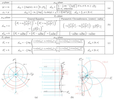
Figure 1. Graphical analysis of the modulus and phase from (a) the ρ-plane to the ρlog-plane — an
example of the curves in Table 1(a) whenφZ0 = 25◦ and (b) from the ρlog-plane to theZn-plane.
3. COMPLEX TRANSFORMATIONS BETWEEN PLANES
Once the log-GSC has been introduced together with the relations betweenρandZnby means of Eqs. (7)
and (6), respectively, the graphical analysis is done by parameterizing the real and imaginary parts, as well as the modulus and phase of each parameter and geometrically studying the resulting curves (the same metodology used in [1] and [5]). The most important transformations may be summarized as follows.
3.1. Analysis of Zn from ρlog
This analysis leads to representingZnalong the TL, studying the reflection coefficient fromρlog instead
of ρ and avoiding the use of Eq. (5). Solvingρlog from Eq. (6),
ρlog =
1 2log
(
1 +ZnejφZ0
1−ZnejφZ0 )
Figure 2. Graphical analysis of the real and imaginary parts from the Zn-plane to the ρlog
-plane conforming the log-GSC.
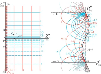
Figure 3. Example of a procedure to relate both theρ- and the ρlog-planes.
and parameterizing the real and imaginary parts ofρlog, leads to the results in Table 1(b) and Fig. 1(b).
The ρ′′log-curves in Fig. 1(b) are π2-periodically overlapped, whereas ρ′log-curves tend to point O when their values decrease. Both are sloped byφZ0 and geometrically connected byφγ in theρlog-plane when
studying them along the TL.
3.2. Analysis of ρlog from ρ
This analysis is carried out parameterizing the modulus and phase ofρas indicated in Table 1(a). Main curves locating points O and A-E in theρ-plane have been transformed into theρlog-plane as shown in
Fig. 1(a). Notice that the ρlog-plane is left-opened when approaching to point O leading to the idea of
being possible to add equal length-scales along the TL.
3.3. Analysis of ρlog from Zn: The log-GSC
Parameterizing the real and imaginary parts of Zn in Eq. (6) leads to the expressions summarized in
Table 1(c) and depicted in Fig. 2. The complexity of the parameterized expressions in Table 1(c) leads to the use of the GSC instead of the log-GSC when composing impedances graphically.
4. EXAMPLES OF USE
Some examples using the log-GSC are presented then in order to remark the usefulness which provide for the analysis of the wave parameters along the TL, operating together with theρ- and Zn-planes.
4.1. Graphical Procedure to Relate ρ- and the ρlog-planes
The convenience of using theρlog-plane instead of theρ-plane has been seen in the analysis of the wave
parameters along the TL.
However, the use of ρlog-plane lacks some facilities provided by the GSC, e.g., the simplicity of
curves — circumferences [1] —- parameterizing impedances from theZn-plane. Thus, a direct graphical
procedure to relate ρ- and ρlog-planes becomes very useful. In this sense, each plane will support the
other emphasizing its own usefulness. In Fig. 3, an intuitive procedure to transformρ- andρlog-planes is
presented in the same graph. Modulus transformations are depicted in red and magenta, whereas phase transformations are coloured in blue and green, and supported by the eye-pattern curves 12log(ρ) and
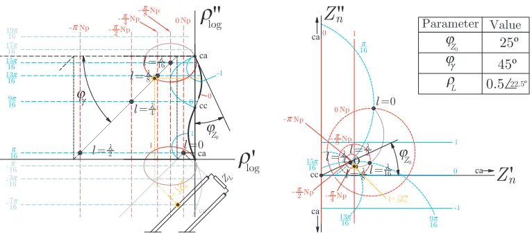
Figure 4. An example of the graphical analysis along the TL using of the ρlog- and Zn-planes.
The example in Fig. 3 shows theρlog-plane usefulness through the characterization ofρalong the TL
leading to adding wavelength scales easily and highlighting some a priori hidden physical interpretations. Notice that the ρlog-plane has been folded, which is possible since φρ ≥ 0 and φρ ≤0 regions do not
overlap each other in theρlog-plane with the exception of their common boundary. Thus, the maximum
and minimum in the folded ρlog-plane (denoted by B’ and C’) are located in the same point. This
compact representation may be useful when trying to relate the log-GSC and the GSC.
4.2. Analysis along the TL
In Fig. 4, the spiral of Eq. (6) in the Zn-plane has been obtained going over the straight line which
represents the TL in the ρlog-plane, as well as adding regular scales in terms of λ. Notice that, since
TL losses are fixed, the curve in the ρlog-plane keeps up the anglesφZ0 and φγ. To the truly physical
realizability of the TL, these angles have to fulfil the following conditions,
0≤φγ+φZ0 ≤ π
2 and 0≤φγ−φZ0 ≤
π
2,
(9)
because of the normalized lossy model proposed [1]. Through the double condition in Eq. (9), the values of r and g are fixed, so the inverse characterization of the TL in terms of the line parameters may be rapidly deduced from theρlog-plane (see the next example concerning matching impedances with lossy
TLs).
4.3. Impedance Matching with Lossy TLs
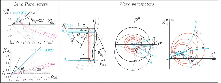
By means of this example, the most practical use of theρlog-plane and lossy TLs matching the impedance ZM from any impedance at the loadZLis pointed out.
The analysis in Fig. 5 follows the procedure: (i) by fixing an arbitraryφZ0 (e.g.,φZ0 = 25◦),ρlogL
and the desiredρlogM are located in theρlog-plane. From this plane, (ii) a straight line representing the
TL length is drawn up linking these points directly, so φγ is obtained (φγ = 63.435◦ in the example).
The phases verify Eq. (9), so the TL is physically realizable assuming the line parameters (r = 0.027 and g= 1.260 in the example). With this parameterization, the analysis in both theρ- and Zn-planes
is completed by transforming the curves from the ρlog-plane (the concrete values of the example are
shown in Fig. 5). It is important to remark how the analysis from theρlog-plane makes the impedance
matching easier by means of a complete graphical process. Notice also that the solution achieved is not unique because of the arbitrary selection of φZ0 and the direct line linking ρlogL and ρlogM, which
provides the shortest TL but not the only one possible. In any case, the analysis in theρlog-plane also
Figure 5. Graphical analysis of the matching procedure from the impedanceZL= 2 + 2j to the real
impedanceZM = 1.5 by using a TL with φZ0 = 25◦ and φγ = 63.435◦.
5. CONCLUSION
A new version of the Smith Chart has been introduced in this paper. The ρlog-plane containing the
log-GSC has demonstrated its usefulness when trying to analyze the wave parameters along the TL. In this sense, some examples of use have been presented taking advantage of the graphical and geometrical analysis along the TL which theρlog-plane gives special emphasis to. Splitting the analysis of lossy TLs
in propagative and evanescent in the ρlog-plane may be specially important in power balance analysis
as well as in the construction of graphical transformations between planes. In addition, by means of the analysis in the ρlog-plane, some practical uses of TLs have been shown taking advantage of the losses
when studying them rigorously, alternative to the classical matching techniques based on lossless TLs.
ACKNOWLEDGMENT
This work has been supported by the Spanish “Econom´ıa y Competitividad” Ministry under projects TEC2014-54005-P and TEC2016-80815-P.
REFERENCES
1. Gago-Ribas, E., Complex Transmission Line Analysis Handbook, Vol. GW-I, “Electromagnetics & Signal Theory Notebooks” series. GR-Editores, Le´on, Spain, 2001.
2. Gago-Ribas, E., P. Vidal-Garc´ıa, and J. Heredia-Juesas, “Complex analysis and parameterization of the lossy transmission line theory and its application to solve related physical problems,”
International Conference on Electromagnetics in Advanced Applications, ICEAA 2015 Proceedings, 141–144, Torino, Italia, September 7–11, 2015.
3. Smith, P. H., “Transmission-line calculator,” Electronics, Vol. 12, 29, 1939.
4. Smith, P. H., “An improved transmission-line calculator,” Electronics, Vol. 17, 130, 1944.
5. Gago-Ribas, E., C. Dehesa Mart´ınez, and M. J. Gonz´alez Morales, “Complex analysis of the lossy-transmission line theory: A generalized Smith Chart,”Turkish Journal of Electrical Engineering & Computer Sciences (Elektrik), Special issue on Electrical and Computer Engineering Education in the 21st Century; Issues, Perspectives and Challenges, Turkey, Vol. 14, No. 1, 173–194, 2006. 6. Wu, Y., Y. Zhang, and Y. Liu, “Analysis of the omnipotent Smith Chart with imaginary
characteristic impedances,”ICMMT 2008 Proceedings, Nanjing, China, April 2014.
7. Wu, Y., H. Huang, and Y. Liu, “An extended omnipotent Smith Chart with active parameters,”