Accurate Evaluation of the Conductor Loss in Rectangular
Microstrip Patch Reflectarrays
Sembiam R. Rengarajan1, * and Richard E. Hodges2
Abstract—In the moment method solution of the integral equations for currents of a rectangular microstrip patch reflectarray, the Leontovich boundary condition is employed to determine the conductor loss. If the basis functions contain edge conditions that approach infinity, the moment matrix elements will have diverging integrals in the Galerkin technique. In this paper, we present a criterion to stop the evaluation of these integrals at a distance before the edge, thereby avoiding the divergence problem. The stopping distance derived here is found to work for a range of values of permittivity, loss tangent, and thickness of the substrate, polarization, angles of incidence of the plane wave source, and also for superstrates. Our computed results are in good agreement with measured results and those computed by HFSS.
1. INTRODUCTION
The design and analysis of reflectarray antennas generally employ an approximate model of an infinite array excited by a plane wave based on local periodicity. The induced currents in the unit cell patch are usually formulated in terms of integral equations and solved by the method of moments (MoM) [1]. A previous work showed that for a rectangular patch, a single basis function with uniform distribution across the current direction and a half sinusoidal variation with an edge condition approaching zero along the current direction in MoM, referred to as MoM1 in this paper, yields good results for the reflection
coefficient [2]. For a very accurate evaluation of the phase of the reflection coefficient, especially for small values of the substrate thickness, a set of basis functions exhibiting even and odd variations and edge conditions approaching zero in the current direction and infinity across the current direction in the MoM solution, referred to as MoM2 here, is required [2]. In both cases, the Galerkin procedure was
employed.
The conductor loss in thin microstrip elements is evaluated in the moment method by using the well-known Leontovich boundary condition wherein one equates the total tangential electric field to the intrinsic impedance of the metal times the surface current [3, 4]. Application of a Galerkin formulation then yields moment matrix elements containing the inner product of identical basis and testing functions, resulting in diverging integrals when edge currents such as those in MOM2 approach infinity. In
prior work, conductor loss could not be incorporated because of these divergent integrals [2]. Lewin encountered similar integrals in analyzing dissipation in microstrip lines with infinite edge currents and was able to circumvent the problem by halting the integral at a distanceδ from the edge and comparing the conductor loss of the thin microstrip line (modeled as a zero thickness line) with that of a finite thickness strip [5]. The procedure for determining the stopping distance δ was generalized to different edge shapes by Barsotti et al. [6]. Following Lewin, to include the conductor loss in MOM2 for more
accurate analysis of reflectarrays, we derive a stopping distanceδ for evaluating the divergent integrals
Received 26 July 2018, Accepted 5 November 2018, Scheduled 11 November 2018
* Corresponding author: Sembiam R. Rengarajan ([email protected]).
1 Department of Electrical and Computer Engineering, California State University, Northridge, CA 91330, USA. 2 Jet Propulsion
by equating the conductor loss calculated in MOM2to that in MOM1The stopping distance thus derived
is found to work for a wide range of parameters of reflectarrays, consisting of rectangular patches in this paper.
2. DIVERGING INTEGRALS
The integral equation for the induced current in a rectangular patch in a unit cell of an infinite array, using the Leontovich boundary condition, is given by
−Es
t +ZmJ=Eti (1)
where E is the electric field, J is the surface current, Zm is the intrinsic impedance of the patch conductor, the subscript t stands for the tangential component and the superscriptss and i stand for the scattered and the incident fields respectively. The scattered field is determined from an integral containing the Green’s function and the patch current [1]. MoM expresses the unknown currents in terms of a set of basis functions and performs the inner product of both sides of (1) with each testing function, which is the same as the basis function in the Galerkin process, thus yielding a set of simultaneous equations. Equations containing the inner product of themth testing function, denoted by the subscript
m, are
−Exs(Jx), Jxm+−Exs(Jy), Jxm+ZmJx, Jxm = Exi, Jxm (2) −Es
y(Jx), Jym+−Eys(Jy), Jym+ZmJy, Jym = Eyi, Jym (3) The basis function for the x-directed electric current in MoM1 is given by
cos(πx/a)[1−(2x/a)2]−1/2 (4)
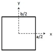
where a is the patch length along x (see Fig. 1). Its width along y is b [2]. The expressions for the
y-directed current has a similar variation with x and a replaced by y and b, respectively. The basis functions for Jx in MoM2 are in the form
cos(mπx/a) sin{(m+ 1)πx/a}
cos(nπy/b) sin{(n+ 1)πy/b}
·[1−(2x/a)2]−1/2[1−(2y/b)2]−1/2 (5)
wherem= 1, 3, 5 etc. andn= 0, 2, 4 etc. It is found that two odd and two even variations along each direction yield excellent accuracy with sixteen unknown coefficients for a non-separable distribution for
Jx. For the y-directed current, the basis functions can be found by replacing x,y,a, andb by y,x, b, and a respectively. In Eqs. (2) and (3) the last term on the left containing the inner product of basis functions and testing functions will diverge for MoM2 whereas it converges for MoM1.
Figure 1. A rectangular patch in the unit cell of an infinite reflectarray.
3. COMPUTED AND MEASURED RESULTS
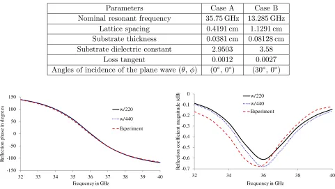
Table 1 shows the parameters of reflectarray antennas discussed in this paper. The stopping distance
Table 1. Reflectarray parameters for two cases.
Parameters Case A Case B
Nominal resonant frequency 35.75 GHz 13.285 GHz Lattice spacing 0.4191 cm 1.1291 cm Substrate thickness 0.0381 cm 0.08128 cm Substrate dielectric constant 2.9503 3.58
Loss tangent 0.0012 0.0027
Angles of incidence of the plane wave (θ,φ) (0◦, 0◦) (30◦, 0◦)
-150 -100 -50 0 50 100 150
32 33 34 35 36 37 38 39 40
R e fl e ct io n ph as e in de g re e s
Frequency in GHz
w/ 220
w/ 440 Experiment
Figure 2. Computed and measured values of the reflection coefficient phase forδ =w/220 and
δ=w/440 (Case A).
-0.7 -0.6 -0.5 -0.4 -0.3 -0.2 -0.1 0
32 34 36 38 40
R e fl ec ti o n c o e ff ic ien t m a g n it u d e ( d B )
Frequency in GHz w/ 220
w/ 440 Experiment
Figure 3. Computed and measured values of the reflection coefficient magnitude forδ =w/220 and
δ=w/440 (Case A).
corresponding result in MoM1. Conductor loss computed by MoM1 has previously been shown to be
accurate [1]. Reflectarray parameters shown in Case A of Table 1 with square patches of side 0.2162 cm were employed in this exercise. The value of δ is found to be w/220, where w, the width is b for Jx and a forJy. Figs. 2 and 3 show the computed values of the reflection coefficient phase and magnitude, respectively, for two different values of δ. The reflection coefficient phase is independent of δ whereas the magnitude decreases withδ. Excellent agreement between computed and measured values is found for the phase in Fig. 2. We found that a value ofδ =w/440 produces a slightly better agreement with experimental results for the magnitude of the reflection coefficient over the frequency band of 32 to 40 GHz in Fig. 3. However, a value of δ =w/220 is used in this work, since it exhibits better results for all cases, including obliquely incident plane waves, discussed later. Theron and Cloete’s calculations for the conductor loss show that the use of Leontovich boundary condition can introduce error, but provides a conservative approximation that is useful in engineering practice [7]. Also, the discrepancy between theory and experiment for the conductor loss is found to be greater than 0.2 dB in [8]. Since the difference between MoM2 and measured or HFSS [9] values of reflection coefficient magnitude is found
to be within 0.1 dB in this work, the conductor loss computed usingδ =w/220 in MoM2 is acceptable
in designs and analyses of reflectarrays. We assumed the ground plane to be a perfect conductor and doubled the surface impedance of the patch, thereby equating the conductor loss in the rectangular patch to that of the ground plane. This simplified procedure, proposed in [3], is justified by the cavity model for a patch antenna [10].
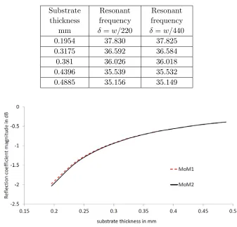
Figure 4 shows the reflection coefficient magnitude at resonance as a function of substrate thickness for Case A. Square patches of side 0.2162 cm were used in this exercise. The resonant frequency given in Table 2 is found to decrease as the substrate thickness increases. A value of δ = w/220 is used in MoM2 in Fig. 4. The magnitude of the reflection coefficient computed by MoM2 is found to be in
Table 2. Resonant frequency in GHz as a function of substrate thickness for two different values of δ (case A in Table 1).
Substrate thickness
mm
Resonant frequency
δ=w/220
Resonant frequency
δ=w/440
0.1954 37.830 37.825
0.3175 36.592 36.584
0.381 36.026 36.018
0.4396 35.539 35.532
0.4885 35.156 35.149
Figure 4. The reflection coefficient magnitude versus substrate thickness for Ka band.
substrate material [2]. The accuracy of MoM1 is known to be poor for thin substrates that exhibit
high values of losses. Computed values of the resonant frequency shown in Table 2 agree to within 0.02% for δ =w/220 and δ =w/440. Reflection coefficient magnitudes computed using δ =w/220 in MoM2 for other values of substrate permittivity, not shown here, also showed good agreement with the
corresponding results of MoM1.
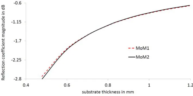
Figure 5 shows the reflection coefficient magnitude at resonance versus substrate thickness for a Ku band reflectarray (Case B in Table 1). The side of each unit cell square patch is 0.542 cm. A TM to z plane wave is incident at an angle ofθ= 30◦ and φ= 0◦.
Experimental results for this reflectarray were used to validate MoM1 and MoM2 for the TE
polarization in a prior work [2]. The value of δ = w/220 used here in MoM2 for oblique incidence
produces very nearly the same values of the reflection coefficient magnitude of MoM1, even though
the stopping distance was determined for normal incidence for the Ka band reflectarray. Figs. 4 and 5 show that the loss increases rapidly as the substrate thickness decreases below approximately 0.066 wavelength in the substrate material since the patches exhibit high quality factor.
Table 3 shows computed results for the resonant frequency and the total loss at resonance for reflectarrays of square patches of side 0.216 cm. All other parameters are specified in Table 1, case A. The results show that the resonant frequencies are independent of the dielectric loss tangent. The total loss computed by the two methods is in good agreement, thereby demonstrating that the stopping distance δ used in MoM2 works for a wide range of values for the dielectric loss tangent as well.
Figure 5. The reflection coefficient magnitude versus substrate thickness for Ku band.
Figure 6. The reflection coefficient magnitude for a reflectarray with a superstrate at normal incidence.
layer of dielectric constant 3.0 and loss tangent 0.001. The square patch size is adjusted to a side length of 0.2025 cm in order to match the 35.75 GHz resonant frequency of the patch without substrate in Fig. 3. MoM2 used withδ =w/220 was also found to provide accurate results in all cases that included
a superstrate. Figs. 6 and 7 show the results for the normal incidence. Figs. 8 and 9 correspond to
θ = 45◦ and φ = 0◦ for TE polarization while Figs. 10 and 11 present the results for θ = 45◦ and
φ= 0◦ for TM polarization. Very good agreement between MoM and HFSS are found for all cases. The
Table 3. Resonant frequency in GHz and total loss in dB as a function of the dielectric loss tangent for reflectarrays (case A in Table 1 with square patches of side 0.216 cm).
Dielectric loss tangent
MoM1 Mom2,δ =w/220
Resonant Frequency
Total loss
Resonant Frequency
Total loss
0.0012 35.92 −0.61 36.03 −0.61
0.005 35.92 −1.20 36.03 −1.18
0.01 35.92 −1.98 36.03 −1.94
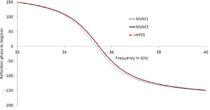
Figure 7. The reflection coefficient phase for a reflectarray with a superstrate at normal incidence.
Figure 8. The reflection coefficient magnitude for a reflectarray with a superstrate for TE polarization at 45◦.
Figure 10. The reflection coefficient magnitude for a reflectarray with a superstrate for TM polarization at 45◦.
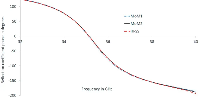
Figure 11. The reflection coefficient phase for a reflectarray with a superstrate for TM polarization at 45◦.
discrepancy between MoM and HFSS for the reflection coefficient magnitude is typically within 0.1 dB in all cases. Results computed using MoM2 are in better agreement with those of HFSS, especially for
the reflection phase.
MoM2 exhibits typically smaller than 0.1 dB lower loss than HFSS for all cases. The resonant
frequencies computed by MoM1 for all cases are within about 0.3% of the value computed by HFSS.
MoM2 is in excellent agreement with HFSS for resonant frequencies. Thus, the choice ofδ =w/220 is
optimum for all cases of substrate thickness, permittivity, dielectric loss tangent, polarization, angles of incident plane waves and for superstrates as well.
4. CONCLUSION
ACKNOWLEDGMENT
The authors wish to thank Dr. Matthew Radway and Dr. Jefferson Harrell for experimental results and Liza Ma for HFSS computations. Dr. Ronald J. Pogorzelski at California State University, Northridge, is thanked for helpful suggestions for the wording of parts of this paper. The research was carried out in part at the Jet Propulsion Laboratory, California Institute of Technology, under a contract with the National Aeronautics and Space Administration.
REFERENCES
1. Pozar, D. M., S. D. Targonski, and H. D. Syrigos, “Design of millimeter wave microstrip reflectarray,” IEEE Trans. Antennas Propag., Vol. 45, No. 2, 287–296, Feb. 1997.
2. Rengarajan, S. R., “Choice of basis functions for accurate characterization of infinite array of microstrip reflectarray elements,”IEEE Antennas Wireless Propag. Lett., Vol. 4, 47–50, 2005. 3. Mosig, J., “Arbitrary shaped microstrip structures and their analysis with a mixed potential integral
equation,” IEEE Trans. Antennas Propag., Vol. 36, No. 2, 314–323, Feb. 1988.
4. Van Deventer, T. E., L. P. B. Katehi, and A. C. Cangellaris, “Analysis of conductor losses in high-speed interconnects,” IEEE Trans. Microw. Theory Techn., Vol. 42, No. 1, 78–83, Jan. 1994. 5. Lewin, L., “A method of avoiding edge current divergence in perturbation loss calculations,” IEEE
Trans. Microw. Theory Techn., Vol. 32, No. 7, 717–719, Jul. 1984.
6. Barsotti, E. L., E. F. Kuester, and J. M. Dunn, “A simple method to account for edge in the conductor loss in microstrip,” IEEE Trans. Microw. Theory Techn., Vol. 39, No. 1, 98–106, Jan. 1991.
7. Theron, I. P. and J. H. Cloete, “On the surface impedance used to model the conductor losses of microstrip structures,” IEE Proceedings on Microwaves Antennas and Propag., Vol. 142, No. 1, 35–40, Feb. 1995.
8. Rajagopalan, H. and Y. Rahmat-Samii, “Dielectric and conductor loss quantification for microstrip reflectarray: simulation and measurements,” IEEE Trans. Antennas and Propag., Vol. 56, No. 4, 1192–1196, Apr. 2008.
9. http://www.ansys.com.