Article
1
Non-Intrusive Load Disaggregation by Linear
2
Classifier Group Considering Multi-Feature
3
Integration
4
Jinying Yu, Yuxin Wu and Chang Su*
5
School of Electric and Electronic Engineering, North China Electric Power University, Changping District,
6
Beijing 102206, China; [email protected] (J.Y.); [email protected] (Y.W.);
7
[email protected] (C.S.)
8
* Correspondence: [email protected]; Tel.: +86-010-61771641 (C.S)
9
Abstract: Non-intrusive load monitoring (NILM) is a core technology for demand response (DR)
10
and energy conservation services. Traditional NILM methods are rarely combined with practical
11
applications, and most studies aim to decompose the whole loads in a household, which leads to
12
low identification accuracy. In this paper, an NILM approach based on multi-feature integrated
13
classification (MFIC) is explored, which combines some non-electrical features such as ON/OFF
14
duration, usage frequency of appliances, and usage period to improve load differentiability. The
15
implementation of MFIC algorithm is consistent with traditional event-based method. The
16
uniqueness of our algorithm is that it designs an event detector based on steady-state segmentation
17
and a linear discriminant classifier group based on multi-feature global similarity. Simulation
18
results using an open-access dataset demonstrate the effectiveness and high accuracy of MFIC
19
algorithm, with the state-of-the-art NILM methods as benchmarks.
20
Keywords: non-intrusive load monitoring; load disaggregation; linear classifier; demand response
21
22
1. Introduction
23
The increased public awareness of energy conservation in recent years motivates electricity
24
consumers to actively participate in energy management [1]. Demand response (DR) is one of the
25
solutions for demand side management, which response to certain conditions by reducing or
26
shifting loads to a different time period. With the advent of smart grid, residential DR has great
27
research potential. Since different types of appliances have different opportunities and ways to
28
participate in DR, it is crucial to study detailed appliance-level power consumption data. In
29
addition, the visualization of detailed consumption of high-power appliances will help customers
30
to replace some inefficient devices, so as to save energy [2].
31
Traditional intrusive load monitoring needs to install large numbers of sensors to acquire
32
signal of each appliance. In the process of sensors’ installation and maintenance, the power supply
33
needs to be temporarily interrupted, causing inconvenience for users. Since the practicability of
34
intrusive method is poor, Hart innovatively proposed the concept of non-intrusive load monitoring
35
(NILM) in the 1980’s [3]. Since its high cost efficiency and less installation effort, NILM is more
36
attractive to customers and utilities. The main idea of NILM is compositing electrical signals at
37
power entrance to track the working status and detailed energy consumption information of
38
individual appliances.
39
Early studies in NILM aim at detecting state-changing event by identifying distinct electrical
40
features of individual appliances, which are called “load signature” and can be divided into two
41
categories: steady-state and transient state. The most common used steady-state signatures are
42
active and reactive power [4-5]. They are effective in identifying high-power devices, but are
43
challenged to separate low-power appliances due to the possibility of power overlap. Later works
44
extended the steady-state signature to many aspects, such as harmonics [6], current and voltage
45
waveforms [7], voltage-current trajectory [8-10], inactive current [11] etc. All of them can effectively
46
disaggregate certain types of appliances. In order to define more accurate load signatures,
47
researchers [12-14] begin to extract features from the period of two stable operations, which is
48
called transient signature. Since transient signatures usually have a relatively shorter duration, the
49
probability of feature overlapping is lower. However, they rely on the samples measured with high
50
rates, so the practicability is limited.
51
With the large-scale deployment of smart meters, NILM approaches that work with lower
52
sampling rate have drawn increasing attention. Most smart meters installed in practical
53
applications measure and transmit the power signals at a relatively low frequency, generally
54
between 1Hz and 1/900Hz [15]. Consequently, the steady-state signatures become a more suitable
55
choice for NILM and have more reality for application. Low-rate NILM methods can be divided
56
into two categories. One is referred as event-based NILM [16], which implements load monitoring
57
by classifying the signatures related to load events. The other is state-based NILM [17], which
58
realizes load disaggregation through pattern recognition.
59
Most of state-based NILM methods are based on Hidden Markov Model (HMM) and its
60
variations [18-21] due to the strong ability in modelling the combination of stationary process with
61
continuous valued data over discrete time. Four different extensions of HMM are presented in [20],
62
but they are likely to converge to a local minimum. To address this problem, Hierarchical Dirichlet
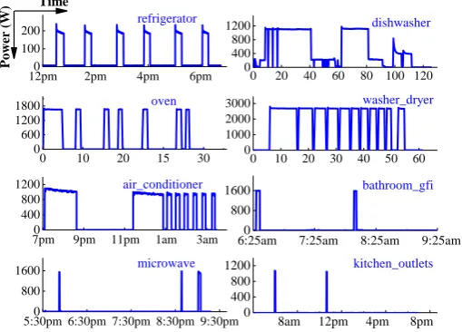
63
Process Hidden semi-Markov Mode (HDP-HSMM) is described in [21]. To extend NILM service to
64
new households without further intrusive monitoring, a model fitting algorithm is designed in [22],
65
which adopts iterative k-means to fit a HMM with only one typical duty cycle of device. The main
66
drawback of HMM is that it is heavily dependent on clean transitions from one state to another,
67
while for continuously varying appliances, the performance is poor. To alleviate this problem, a
68
sparse coding method based on structured prediction is developed [23]. Motivated by the success of
69
deep learning, a deep sparse coding is proposed in [24]. However, a typical shortcoming is that for
70
going deeper, more parameters need to be learned. Additionally, state-based algorithms have a
71
common drawback, i.e., long periods of training and high computational complexity, which makes
72
them difficult to be applied to real-time decomposition.
73
Event-based algorithms have a relatively fixed processing procedure, including event
74
detection, feature extraction and event classification. To obtain accurate identification results,
75
different classification techniques are tried, including k-means [25], k-Nearest neighbour (k-NN)
76
[26], naïve Bayes [27], maximum likelihood [28] and decision tree (DT) [29]. In [28] the maximum
77
likelihood classifier is designed to disaggregate load based on the power profiles, but it only works
78
for single-state loads. Reference [29] relies on graph signal processing (GSP) to perform edge
79
detection, clustering, and pattern matching. However, experimental results show that power
80
fluctuation or close power range of appliances will influence algorithm performance. A novel
81
combined k-means-SVM-based NILM method is developed in [30]. However, event-based methods
82
face a common challenge, that is, most of the existing algorithms only rely on a two-dimensional
83
feature space of active and reactive power for load identification without considering other
84
additional features, such as time and sequence signatures. In addition, the same type appliances in
85
different households have quite different signatures, so it is not suitable to use a unified model to
86
represent them.
87
The existing NILM methods have been focused on detection of all appliances without
88
considering the applicability of load disaggregation in realistic application, that is, there is no
89
definition of an accurate load space related to the actual application. Since the original load space is
90
too complex, it is impractical to identify all devices based on one-dimension aggregate signal.
91
Consequently, in order to jump out of the dilemma of traditional NILM study, it is necessary to
92
combine it with practical application to define a suitable load space.
93
In order to address the difficulty of identifying appliances with similar power, a linear
94
discriminant classifier group considering multi-dimensional features is designed in this paper. It is
95
an event-based method, which can work seamlessly with Smart Meter Infrastructure without
96
provide appliance-level information for DR and energy-saving service, the load space to be
98
monitored can be narrowed down to some controllable and high-power devices.
99
This work formalizes a load identification technique based on the multi-feature integrated
100
classification (MFIC), where the only input is the time-stamped power readings from the smart
101
meter. The major contributions of this paper are 3-fold, which are listed as follows:
102
(1) Considering the different operating habits and inherent electrical characteristics of loads,
103
multi-dimensional features are used to model each appliance and improve the load differentiability.
104
In addition, due to the great difference of appliances signatures in different households, this paper
105
uses proprietary model database to replace the uniform feature database.
106
(2) An event detector based on steady-state segmentation is designed, which has fewer
107
parameters and is independent of the detection window.
108
(3) Based on the overall similarity of multi-features, a linear discriminant classifier for each
109
appliance is designed, which constitutes a linear discriminant classifier group.
110
The structure of this paper is given as follows. Section 2 selects multi-dimensional features for
111
load modelling. In addition, a brief analysis of DR and energy-saving services is made to specific
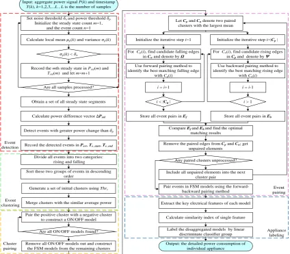
112
the research objective and narrow down the load space. Section 3 elaborates on the problem
113
definition and the complete process of proposed MFIC algorithm. Section 4 presents experiments
114
and their results discussion. The last section concludes the paper and discusses future works.
115
2. Appliance modelling
116
2.1 Appliance Behaviour Modelling
117
The foundation of NILM is to establish an exclusive appliance model library for each user.
118
Therefore, exploiting and defining adequate distinguishable features to model appliance behaviour
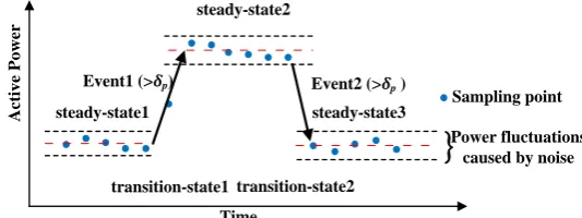
119
is an important preparation work for NILM. Since low-frequency electrical signals contain less
120
detailed features, most of the existing low-rate NILM studies rely solely on power metrics to
121
characterize an appliance. However, the power values of some appliances are very close, so the
122
accuracy is low only using power features to identify. Through the analysis of the concrete
123
operation process of each appliance, some distinguishing features can be found. The power
124
consumption of several typical appliances is shown in Figure. 1.
125
12pm0 2pm 4pm 6pm
100 200
0 20 40 60 80 100 120 0
400 800 1200
0 10 20 15 30
0 600 1200 1800
0 10 20 30 40 50 60 0
1000 2000 3000
7pm0 9pm 11pm 1am 3am 400
800 1200
6:25am0 7:25am 8:25am 9:25am 800
1600
5:30pm 6:30pm 7:30pm 8:30pm 9:30pm0 800
1600
8am 12pm 4pm 8pm --0
400 800 1200
bathroom_gfi air_conditioner
kitchen_outlets microwave
washer_dryer oven
dishwasher
Time
P
o
wer
(
W) refrigerator
126
Figure 1. Load profiles of eight typical appliances
127
Figure.1 presents load profile of the refrigerator between 12pm and 7pm. Refrigerator
128
represents a kind of load with fixed operating period and fixed intermittent time. Without
129
considering the opening of the door, refrigerator operates in a periodic cycle with 15-minutes ON
130
and 51-minutes OFF. A complete operation cycle of the dishwasher can be divided into three main
131
structure. Oven is also an intermittent running load, but unlike refrigerator, the ON-duration and
133
OFF-duration are not fixed. Generally, the operation time of oven is between 15 minutes and 1 hour,
134
depending on the users’ setting. Observing the load profile of washer dryer, it can be found that the
135
first ON time is always the longest, following by several ON/OFF cycles. The number of ON/OFF
136
cycles is related to laundry loads.
137
In this work, we select the following eight features that can be divided into two categories, i.e.,
138
intrinsic features and statistical features. Intrinsic features, also known as electrical features, are
139
generated by the internal structure of appliances. Statistical features reflect users’ habits of using
140
specific appliances, which can be called non-electrical features.
141
Intrinsic features include the following four criteria:
142
Active power change. Note that there is an obvious step change in the load profiles given in
143
Figure.1. It refers to the event brought about by the state transition of appliances, and appears
144
as the rising or falling edge. The typical appliances can be divided into three types: single-state,
145
continuous varying and multi-state. The single-state load has a pair of identical rising/falling
146
edges and constant power consumption between them, such as microwave. However, a
147
continuous varying load such as refrigerator generally has a pair of different rising/falling
148
edges and the power consumption during operation is continuously changing. Besides,
149
multi-state load has more than one working stage, such as dishwasher.
150
On-duration. It refers to the continuous operating time in a periodic cycle. It is mainly applied
151
to the loads with fixed operating periods, such as refrigerator. As abovementioned, the
152
On-duration of the refrigerator is 15 minutes.
153
Off-duration. Similar to the On-duration, Off-duration stands for the continuous standby time
154
in a periodic cycle. For instance, the On-duration of refrigerator is 51 minutes.
155
On times. It means the number of turning on contained in each operation cycle.
156
Statistical features serve to emphasize the user's operating habits for different appliances,
157
including the following four kinds.
158
Switching-time. It refers to the possible switching on/off time, which is related to the function
159
of an appliance.
160
Usage frequency in one day. It is the possible usage count for a day. Notice that there are many
161
appliances operate in an ON/OFF cycle such as oven, air conditioner and washer dryer. When
162
calculating the usage frequency of these loads in a day, it is necessary to ensure that a complete
163
operation process is counted once.
164
Working days in a week. It means the number of days that an appliance may work within a
165
week. A refrigerator is a constant-opening device. But the washing machine is less likely to be
166
used every day.
167
Duration of a complete use process. This feature is used to record the duration of an appliance
168
from start to shut down, including all subsequences ON/OFF cycles. It should be noted that if a
169
load has the habit of operating multiple times in a short time, but their final task is identical, so
170
they can be summed up as a complete operation. For instance, the users may use the stove
171
several times during cooking.
172
2.2 Determine the load space to be monitored
173
As described in the introduction, it is impractical to identify all types of appliances using only
174
one NILM approach, so it is essential to build a reasonable load space according to the specific
175
application of NILM.
176
The opportunities for various appliances to participate in DR are different. They are usually
177
divided into three categories: uncontrollable load (UCL), transferable load (TL) and interruptible
178
load (IL). UCL refers to the load that has no energy storage capacity and may be opened at any time.
179
Its power fluctuation range is small and basically has no capacity to transfer load. However, TL has
180
the ability of load transfer, because its using time is more flexible and the total energy consumption
181
is certain, such as the washing machine and the timed electric rice cooker. Consequently, under the
182
the running time. Air conditioner and water heater are typical IL, which can be interrupted at certain
184
time to reduce the power consumption. Therefore, these loads can usually be interrupted
185
temporarily without resulting in consumer discomfort. In summary, TL and IL can participate in
186
DR, and can be monitored and managed centrally at the control center. On the contrary, the
187
interruption of UCL is likely to affect user’s comfort, so UCL is allowed to be centrally controlled
188
only when emergency occurs.
189
Above analysis specifies the load space that NILM should focus on when providing services for
190
DR. The main research target is to identify the high-power and adjustable loads, while there is no
191
need to track the appliances with small power. The load space that needs to be monitored is
192
narrowed down, only including some controllable loads (IL and TL) or high energy consumption
193
loads without adjustable ability. The final load space to be monitored is reported in Table 1.
194
Table 1. Load space to be monitored.
195
Types Loads
IL or TL
HVAC (Heating, Ventilation and Air Conditioner), Electric Heat loads (water heater, furnace, oven), electric vehicle
charger, washer and dryer, dishwasher, refrigerator
UCL High-power devices
3. Methodology
196
3.1 Load Disaggregation Definition
197
The definition of load decomposition can be expressed as follows: Given the mixed signal
198
collected at the entry point of a house and typical appliance models in it, we need to breakdown the
199
mixed signal into a set of individual components that are attributed to specific appliances.The
200
composite signal is clearly depending on which appliances are switched ON at the given moment,
201
so it is necessary to design a Boolean coefficient an,m(k), which determines whether the mode m of
202
appliance n is ON at the kth sampling point. Mathematically, the observed mixed signal can be
203
formulated as a linear combination of some unknown appliance load profiles.
204
, ,
1 1
( ) N M n m( ) n m( ) ( )
n m
P k
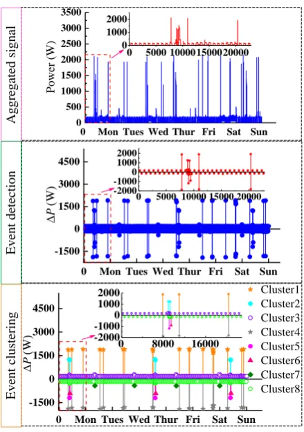
a k p k e k (1)where P(k), k=1,2,3,…,L is the aggregated power signal (L is the number of samples) and pn,m(k)
205
denotes the individual power consumption of appliance n in mode m. N and M are the number of
206
appliances and modes, respectively. e(k) stands for the noise signal and small appliances, including
207
phone chargers, DVD player and laptop computers. In load identification, e(k) is ignored. In other
208
words, the objective in NILM is to decode P(k) and obtain the status of each appliances using a set
209
of appliance models in the house.
210
In existing research, combinatorial optimization is a common method to solve (1), which finds
211
the optimum appliance status by minimizing the difference between the actual aggregate power
212
and the sum of disaggregated appliance powers, subject to some prior information.
213
,
, 1 1 , ,
( )
( ) arg min ( ) ( ) ( )
n m
N M
n m n m n m n m
a k
a k P k a k p k
(2)
3.2. Algorithm overview
214
There will be many uncertainties in reality, because different appliances may perform similar
215
electrical signature “power”. Appliances may not operate at its rated power, because the actual
216
power consumption is proportional to the total load. Therefore, it is difficult to solve the problem in
217
(2) by combinatorial optimization.
218
The actual electric data displays that it is easy to segment the total signal into some
219
steady-state process by clearly step changes. Therefore, an event-based algorithm is designed in this
220
detection and clustering, 2) event paring and key electrical feature extraction and 3) feature
222
matching. In the first step, we make statistics on the significant changes in active power, which
223
represent that some appliances have changed their status. Then, events with similar power should
224
be grouped, i.e., clustering. After the formation of clusters, events in “positive” clusters should be
225
paired with those in negative clusters. Finally, extract the key features from each positive-negative
226
cluster pair, and match with the appliance models. The flowchart is illustrated in Figure.2.
227
Input: aggregate power signal P(k) and timestamp T(k), k=1,2,3,...L , L is the number of samples
Calculate local mean μp(k) and variance σp(k)
Record the mth steady state in Pstd(m) and Tstd(m) and let m=m+1
Are all samples processed? Set noise threshold δn and power threshold δp
Initialize the steady state count m=1, and the event count n=1
Obtain a set of all steady state segments
Calculate power difference vector ΔPstd
Detect events with greater power change than δp
Record the detected events in Pevt, Te_start, Te_end
Divide all events into two categories: rising and falling
Sort these two groups of events in descending order
Generate a set of initial clusters using Thrc
Merge clusters with the similar average power
Pair the positive cluster with a negative cluster to construct a ON/OFF model
Are all ON/OFF models found?
Remove all ON/OFF models out and construct the FSM models from the remaining clusters
σp(k) < δn
Include all unpaired elements into the next cluster pair
Pair events in FSM models using the forward-backward pairing method
Extract the key electrical features of each model
Calculate similarity index of single feature
Label the disaggregated models by linear discriminate classifier group
Output: the detailed power consumption of individual appliance Let CpandCndenote two paired
clusters with the largest mean
For Cp(i), find candidate falling edges in Cnand denote by Ω
Use forward pairing method to identify the best matching falling edge
with Cp(i)
For Cn(i), find candidate rising edges in Cp and denote by Ψ
Remove the paired edges from CpandCn; get
unpaired elements i < |Cp |
Initialize the iterative step i=1
i = i+1
Store all event pairs in Ef Store all event pairs in Eb
Compare Ef and Eb and find the optimal
matching results
Any paired clusters unprocessed?
Initialize the iterative step i=|Cp|
Use backward pairing method to identify the best matching rising edge
with Cn(i)
i = i-1
i > 1
Event detection
Event clustering
Cluster pairing
Event pairing
Appliance labeling
228
Figure 2. Flowchart of the proposed algorithm
229
3.3. Steady-state Segment Based Event Detection
230
One important characteristic of event-based load disaggregation is to detect the significant
231
rising or falling edge in active power, and record the power value and occurrence time of events. A
232
steady-state segment based event detection method is presented. It has two parameters, one is the
233
noise threshold dn, the other is the power threshold dp. The schematic diagram of the event detection
234
is indicated in Figure.3.
235
Each appliance can be represented by two states: 1) steady state, including both ON state and
236
OFF state; and 2) transition state, i.e., the process of switching ON/OFF or changing operation state
237
of multi-state appliance. As long as the steady-state segments have been identified, the duration of
238
the power-on or power-off processes for different appliances can be determined adaptively. Based
239
on the switch continuity principle proposed in [3], we can suppose that load switching is successive,
240
i.e., only one state transition can occur within the sampling time interval. Thus, it is feasible to use
241
Power fluctuations caused by noise steady-state1transition-state1
steady-state3
transition-state2 steady-state2
Event2 (>δp )
Event1 (>δp)
A
c
ti
v
e
P
o
w
e
r
Time
Sampling point
243
Figure 3. Schematic diagram of the event detection
244
On the one hand, the power grid noise exists always in the actual electric environment. On the
245
other hand, the time of state transition can be longer than the sampling interval. Consequently, it is
246
necessary to design an appropriate event extraction method, which is robust to the possible
247
variation of power amplitude due to sampling and noise. We adopt the method of calculating local
248
mean and variance to find steady state. Assuming P(k), k=1,2,3,…,L is a given aggregate power
249
signal and T(k), k=1,2,3,…,L is the corresponding timestamp, two quantities need to be calculated by
250
equation(3) and (4), the former is the local average power and the latter is the local variance.
251
1 1 1
( ) ( )
3
P k i P k i
(3)1 2
1 1
( ) 3 ( ( ) ( ))
P k i P k i P k
(4)Let n2 denote the noise variation in power grid. If p(k)<n, P(k) is considered to be in a steady
252
state and then two new variables Pstd(m) and Tstd(m) are added to record the mth steady state, i.e.,
253
( ) ( )
std P
P m k (5)
( )
std
T m k (6)
After all the steady state segments have been identified, the power difference between two
254
consecutive steady states will be calculated as follows:
255
( ) ( ) ( 1)
std std std
P m P m P m (7)
Given the power threshold p, it is set by users and denotes the events they are interested. For
256
example, if users want to find events with power change greater than 100 W, they will set p=100. If
257
abs(△Pstd(m))> p, it indicates that a new event is detected and the power value and timestamp of
258
this event will be registered as
259
( ) ( )
evt std
P n P m (8)
_ ( ) ( ( 1))
e start std
T n T T m (9)
_ ( ) ( ( ))
e end std
T n T T m (10)
where n represents the nth event. Pevt(n) stands for the power value of the nth event, Te_start(n) and
260
Te_end(n) stands for the start time and end time of the event respectively.
261
3.4. Event Clustering
262
The collection of the registered events Pevt(n), n=1,2,…,Ne is the basis of the event clustering. Ne
263
denotes the number of events detected. Since we assume that each state of appliances has a unique
264
value and only one appliance may have state transition in one sampling interval, it is reasonable to
265
gather events with similar value into one cluster. Ideally, each cluster represents one kind of state
266
In this paper we design a clustering algorithm without prior knowledge, which can adaptively
268
determine the number of clusters. There are two steps in this algorithm.
269
Step 1) Separate the rising and falling edges of the event candidates into two collections of
270
Pevt_up and Pevt_down. Then the rising and falling edges are arranged in descending order according to
271
the absolute value of power respectively. Set a cluster threshold Thrc. When the difference between
272
two consecutive rising or falling edges is greater than Thrc, a new cluster is generated. Here we set
273
Thrc smaller so that the clustering results will be more detailed. However, it is also easy to separate
274
some events with power fluctuation but belonging to one appliance into different clusters. In order
275
to solve this problem, we merge some clusters with the similar average power. The detailed process
276
is illustrated in step 2.
277
Step 2) Calculate the mean power of each cluster, and gain the mean power difference between
278
two adjacent clusters. If the difference is less than a certain value, it can be considered that these
279
two adjacent clusters belong to the same appliance state. Thus, we will merge them together and
280
the new cluster candidates will be formed.
281
3.5. Building Appliance Candidate Model
282
After clustering the events, we get some “positive” clusters containing rising edges and
283
“negative” clusters composed of falling edges. Next, the pairing method is designed to
284
automatically generate appliance candidate models.
285
Most of the existing NILM algorithms only consider the single-state appliances, but in practice,
286
the multi-state appliances are very common. These appliances cannot be described by ON/OFF
287
model, so it is necessary to establish an appropriate model for them. The finite state machine (FSM)
288
[1] is a typical model for these appliances. The sum of power changes in any cycle of state transition
289
is zero, which can be called Zero Loop-Sum Constraint (ZLSC) [1]. Besides, different operating
290
states in an FSM model have different power levels, i.e., Uniqueness Constraint (UC). The two
291
constraints make it possible to construct individual FSM from streams of events.
292
In the following, the method of generating ON/OFF or FSM models is introduced. It includes
293
two main steps, i.e., cluster pairing and event pairing.
294
Step 1) To construct ON/OFF models for the single-state appliance candidates, all we need to
295
do is pairing the “positive” cluster and “negative” cluster with similar absolute average power.
296
However, the construction of FSM models is somewhat complex, which should take advantage of
297
special algebraic properties of events in a complete transition cycle, i.e., ZLSC and UC. In order to
298
reduce the complexity of cluster pairing, the ON/OFF models are built firstly. After all
299
positive-negative cluster pairs have been found, we remove them from the total clusters and search
300
for FSM models from the remaining clusters.
301
Step 2) Following the cluster pairing, some cluster pair candidates for single-state or finite-state
302
appliances will be generated. Then, it is essential to further match the events in each cluster pair.
303
That is to say, looking for the complete state transition processes of each appliance candidate. For
304
example, we need to match each rising edge in the positive cluster with a falling edge in the paired
305
negative cluster, exploiting power difference and time intervals between two events as pairing
306
features. Next we will focus on the event pairing process of ON/OFF models, which is also
307
applicable to the FSM model. In order to increase pairing accuracy, a specialized forward-backward
308
pairing procedure is designed.
309
Let Cp and Cn denote two paired clusters, where |Cp| and |Cn| denotes their cardinality.
310
(a) Forward Pairing
311
The goal of forward pairing is, for each Cp(i)∈Cp, match an optimal falling edge among all
312
elements in Cn according to the order from i=1 to |Cp|-1. Normally, the ON and OFF events appear
313
alternately, that is, using time stamps to sort events that belong to the same appliance will get an
314
ON/OFF/ON/OFF… sequence. Thus, the falling edge paired with Cp(i) must occur after Cp(i) and
315
before Cp(i+1). The subset of Cn that satisfy the above condition is considered as a set of candidates,
316
three cases. Different pairing processes are designed for these cases. Define two vectors Mp and Mt
318
to record the power difference and time intervals between paired events.
319
Case 1: When |Ω|=1, the absolute power difference and time interval between Cp(i) and the
320
only element in Ω are calculated and denoted by Ωp and Ωt respectively. Then the probability of
321
pairing Cp(i) and the element in Ω can be defined as:
322
2 2 2 2
( )( )
p p t t
i
p t p t
m m
c
m m
(11)
Where, mp stands for the mean value of the elements in Mp and mt denotes the median value of the
323
elements in Mt.
324
If ci is larger than a given threshold, the only element in Ω can be considered as the paired
325
falling edge for Cp(i), otherwise they are not match. Then record Ωp and Ωt between paired events in
326
vector Mp and Mt.
327
Case 2: When |Ω|>1, the absolute power differences and time intervals between Cp(i) and each
328
candidate in Ω are calculated and denoted by Ωp and Ωt respectively. Then the probability of
329
pairing Cp(i) and the jth candidate in Ω can be defined as:
330
2 2 2 2
( ) ( )
( )
( ( ) ( ) )( )
p p t t
i
p t p t
j m j m
c j
j j m m
(12)
Find the falling edge Cn corresponding to the maximum value in vector ci. If the maximum
331
value is larger than the given threshold, Cn can be judged to the paired falling edge for Cp(i). Then
332
record the power difference and time intervals between paired events by vector Mp and Mt.
333
Case 3: When |Ω|=0, we think there is no appropriate element in Cn pairing with Cp(i).
334
However, it is not applicable to a special situation, i.e., Cp(i+1) is wrongly cluster. In this case, the
335
accuracy of the results obtained by forward pairing is lower, so backward pairing is proposed.
336
When the forward pairing is complete, all event pairs are stored in matrix Ef.
337
(b) Backward Pairing
338
The goal of backward pairing is, for each Cn(i)∈Cn, match an optimal rising edge among all
339
elements of Cp according to the order from i=|Cn| to 2. According to the analysis in forward pairing,
340
the rising edge paired with Cn(i) must occur before Cn(i) and after Cn(i-1). The subset of Cp that
341
satisfies the above condition is considered as a set of candidates, denoted by Ψ. Let |Ψ| represent
342
the element number of Ψ. The specific realization process is basically the same with the former
343
pairing. However, it is worth noting, that when |Ψ|=0 the accuracy of the results obtained by
344
backward pairing is lower, which needs to be analysed with forward pairing results. When the
345
forward pairing is complete, all event pairs are stored in matrix Eb.
346
Finally, comparing Ef and Eb, we can find the optimal matching results. The event pairs that
347
appear in both Ef and Eb are thought to be matched correctly. If there are some event pairs in Ef and
348
Eb that have the same rising edges but the corresponding falling edges are different, then the
349
pairing results in Ef are considered to be optimal. The essence of this situation is that there are
350
multiple falling edges between two successive rising edges, leading to inaccurate results of
351
backward pairing. Moreover, if there are some event pairs in Ef and Eb that have the same falling
352
edges but the corresponding rising edges are different, then the pairing results in Eb are considered
353
to be optimal. The essence of this situation is that there are multiple rising edges between two
354
successive falling edges, leading to inaccurate results of forward pairing.
355
3.6. Appliance Identification Based on Multi-feature Integrated Classification
356
With the aforementioned process, the raw smart meter recordings are decomposed to a set of
357
appliance candidate models and each model carries unique information that corresponds to an
358
appliance footprint. Next, the key features are extracted to label each candidate model combined
359
3.6.1. Similarity Index of Single Feature
361
Intrinsic features are determined by the internal structure of appliances, which are not affected
362
by the user's behaviour habits, and usually expressed as fixed values without some small
363
fluctuations caused by the grid noise. The similarity indices of these features can be quantified as
364
( )( ) exp
( )
mean
mean v v
S v k
H v v
(13)
max mean
min mean
, Δ 0 (Δ )
, Δ 0
v v v
H v
v v v
(14)
where (·) denotes the intrinsic feature of detection. v represents the detected value of certain feature
365
and vmean is the average value of certain feature recorded in the feature library. Considering the
366
noise in appliances or power grid, there are some small fluctuations in these intrinsic features, so
367
vmax and vmin are used to represent the limits of up and down fluctuation respectively. H(·) is a
368
piecewise function. k is a calibration parameter to ensure that when the detected value v exceeds
369
vmax and vmin, its similarity index is almost 0. In this paper, k=1 is used.
370
Statistical features are expressed as a range rather than a fixed value. The similarity calculation
371
of statistical features is defined as
372
( ) ( )
( ) 1, ( )
0,
x R
S x
x R
(15)
where (·) denotes the statistical feature of detection. x is the statistical value of specific feature. R(•)
373
stands for the range of possible values for a certain feature.
374
3.6.2. Appliance Recognition Based on Linear Discriminant Classifier Group
375
The task of this section is to label each appliance candidate model based on similarity indices.
376
In order to synthetically consider the effects of various features on appliance identification, a linear
377
discriminant classifier is designed for each appliance based on the overall similarity and all of them
378
constitute a linear discriminant classifier group. Overall similarity is calculated by weighted
379
composition. The features of marking different appliances are inconsistent. Therefore, the particular
380
weight vector needs to be set for each linear discriminant classifier separately. It is firstly estimated
381
by observing the identifiability of different features. For instance, knowing refrigerator has specific
382
ON-duration and OFF-duration, these two features will be emphasized. But they are insignificant in
383
lights identification, which can range from a few minutes to a whole day. Generally, the intrinsic
384
features are important than statistical features since statistical features are easily influenced by
385
external environment. For multi-state appliances, the sequence feature is particularly important.
386
After the weight vectors are predefined, it is necessary to adjust their values exploiting the test data
387
in different time and environment, so as to ensure recognition accuracy.
388
The detailed process of labelling appliance candidate models is described below. At first, the
389
intrinsic and statistical features of each model are extracted. Then each unlabeled model will be
390
classified by the linear discriminant classifier group in this particular house. The classification result
391
of the jth classifier is shown as
392
( ) T
j j j j
d S ω S
(16)where ωj is the weight vector of the jth classifier, Sj includes feature similarity indices between the
393
unlabelled model and the jth classifier, and δj represents the judgment threshold of the jth classifier.
394
If d(Sj)>=0, the unlabelled model is determined as the appliance corresponding to the jth classifier;
395
Otherwise not.
396
4. Experiment and result analysis
In order to verify the effectiveness of the proposed algorithm, simulation experiments are
398
carried out using the low-frequency database: REDD [31]. It is one of commonly used database in
399
the field of NILM, so testing our method with it allows better comparison with other approaches.
400
4.1. Performance Metrics
401
In order to evaluate the performance of separated signals and compare existing implemented
402
algorithms, some indices are needed to calculate the performance quantitatively. Since an
403
event-based NILM algorithm is designed in this paper, it is essential to measure the accuracy of this
404
method in predicting what appliance is running in each state. Classification accuracy indices, such
405
as precision, recall, and F-measure, are well suitable for this task. Precision denotes the positive
406
predictive values, i.e., the correct proportion of samples identified as appliance c. Recall represents
407
the true positive rate, i.e., the proportion of samples belonging to appliance c that are recognized
408
correctly. F-measure is harmonic mean of precision and recall. These typical classification metrics
409
can be formulated as follows:
410
/ ( )
c c c c
P TP TP FP (17)
/ ( )
c c c c
R TP TP FN (18)
2 ( ) / ( )
c c c c c
F PR PR (19)
where, the subscript c is used to mark different appliances or states. TPc indicates true positive, i.e.,
411
the correct judgment that appliance c was ON, FPc represents the false positive, i.e., judged
412
appliance c was ON but actually was OFF, FNc denotes false negative, that is, appliance c was ON
413
but was wrongly judged as OFF. Note that these indices (TPc, FPc, FNc) are accumulations over a
414
certain experimental time period.
415
On the other hand, it is important to feedback the detailed power consumption of each
416
appliance to users, so the accuracy based on power estimated also needs to be considered. The
417
frequently used measures to compare the estimated power with the actual power consumption
418
include disaggregation accuracy (DA), disaggregation error (DE) and percentage of contribution in
419
energy consumption (PCEC). The first two metrics provide a global comparison between the
420
estimated power and the ground truth, while PCEC is used to calculate the contribution of each
421
appliance in total power consumption. In this paper, DA and PCEC are exploited to evaluate the
422
ability of different algorithms for reconstructing power profiles.
423
1 1
1 ˆ
| ( ) ( ) | 1
2 ( )
L N
n n
k n
L k
p k p k
DA
P k
(20)where L is the number of disaggregated readings, N denotes the number of appliances in the house,
424
ˆ ( )n
p k represents the estimated power consumption of appliance n at the kth sample, pn(k) is the
425
actual power consumed at the kth sample for appliance n, and P(k) stands for the aggregate power
426
measured at the kth sample.
427
1ˆ ( ) / 1 ( )
L L
n
n
k k
PCEC
p k
P k (21)where PCECn represents the contribution of appliance n to total power consumption.
428
Furthermore, energy usage profile pie graph and comparison curve between disaggregated
429
signals and their ground truth are other means to verify the performance of different algorithms.
430
4.2. Case Study 1
431
Several appliances are selected from House 2, namely refrigerator, microwave and dishwasher.
432
Refrigerator and microwave are used frequently and have high power consumption in this house.
433
depends on some statistical features, the aggregate power signals in one week are selected for the
435
experiment. Figure.4 shows the results from aggregate signal to event detection and clustering.
436
0 Mon Tues Wed Thur Fri Sat Sun
0 500 1000 1500 2000 2500 3000 3500
0 5000 100001500020000 0
1000 2000
0 Mon Tues Wed Thur Fri Sat Sun -1500 0 1500 3000 4500 Cluster1 Cluster2 Cluster3 Cluster4 Cluster5 Cluster6 Cluster7 Cluster8
0 8000 16000
-2000 -1000 0 1000 2000 A g g re g at ed s ig n al E v en t d et ec ti o n E v en t cl u st er in g P o w er ( W ) P ( W )
0 Mon Tues Wed Thur Fri Sat Sun -1500
0 1500 3000 4500
0 5000 10000 15000 20000
-2000 -1000 0 1000 2000 P ( W )
437
Figure 4. Results of event detection and clustering for House 2
438
Figure.4 illustrates the results of event detection and clustering in one week. In order to show
439
the process more clearly, the results in Monday are expanded and reported in Figure.4. Using the
440
steady-state segment based event detection method, the significant changes from aggregate power
441
signal can be detected accurately. After processing all events with the proposed clustering method,
442
eight different clusters are formed, including three “positive” clusters and five “negative” clusters.
443
It can be seen that the elements in each cluster have similar power value.
444
0
MonTuesWedThur Fri Sat Sun
-2000 -1000 0 1000 2000 0
MonTuesWedThur Fri Sat Sun
-200 -100 0 100 200 0
MonTuesWedThur Fri Sat Sun
-300 -150 0 150 300 0
MonTuesWedThur Fri Sat Sun
-1200 -600 0 600 1200
0 Mon Tues WedThur Fri Sat Sun
-1000 -500 0 500 1000 1500 O N /O F F m o d el F S M m o d el
model 1 model 2
model 3 model 4
model 5
445
Figure 5. Results of event pairing for House 2
446
Next, each positive cluster is matched to the magnitude-wise closest negative cluster with the
447
cluster pairing method. Then for each cluster pair, the forward-backward pairing approach is
448
through the remaining unmatched events, until no events can be matched. After each loop, all
450
positive-negative cluster pairs that have completed the matching process will be stored as the
451
ON/OFF models, passed to the following appliance identification step. When all ON/OFF models
452
have been found, we remove them from the set of events and attempt to establish FSM models from
453
the remaining events. Figure.5 presents the results of building appliance candidate models. Four
454
ON/OFF models and one FSM model are established, and their corresponding time profile features
455
are shown in Figure.5. It should be emphasized that although the power values of model 3 and
456
model 4 are close, they can still be separated due to the large difference in the ON duration.
457
Finally, the linear discriminant classifier group of house2 is used to label each candidate model
458
and the results of each classifier are reported in Table 2. It can be seen that the classifier group of
459
house 2 consists of seven appliances, namely kitchen outlets, stove, microwave, high-power state of
460
dishwasher, low-power state of dishwasher, multi-state of dishwasher and refrigerator. They are
461
typical loads with high power consumption or adjustable potential in house2, which are interested
462
by users and registered in feature database. Note that different modes of dishwasher with different
463
operation cycles are treated as separated appliances. Therefore, in the final labelling stage, the
464
models that are identified as appliance 4, 5 and 6 are all labelled as a dishwasher. From the signs of
465
classifier value, model 1 is determined as appliance 3 while model 2 is appliance 4 since their
466
corresponding values are greater than 0. In addition, model 3 and 4 represent appliance 7 and 5,
467
respectively. The disaggregated FSM model 5 corresponds to appliance 6. If there is no positive
468
value for a model, it means that the model is caused by an unregistered appliance in the feature
469
database, which may be a new or low power consumption appliance not interested by users.
470
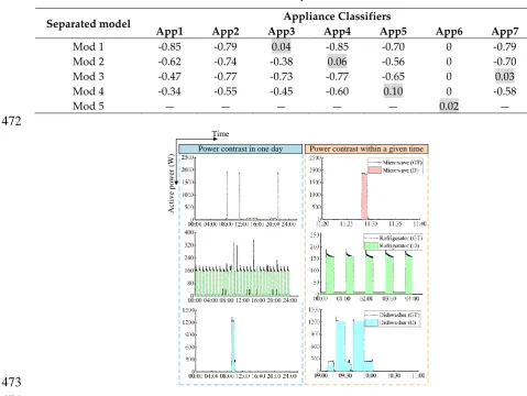
Table 2 Identification results of separated candidate models.
471
Separated model Appliance Classifiers
App1 App2 App3 App4 App5 App6 App7
Mod 1 -0.85 -0.79 0.04 -0.85 -0.70 0 -0.79
Mod 2 -0.62 -0.74 -0.38 0.06 -0.56 0 -0.70
Mod 3 -0.47 -0.77 -0.73 -0.77 -0.65 0 0.03
Mod 4 -0.34 -0.55 -0.45 -0.60 0.10 0 -0.58
Mod 5 — — — — — 0.02 —
472
A
ct
iv
e
p
o
w
er
(
W
) Power contrast in one day Power contrast within a given time
Time
473
Figure 6. Ground truth (GT) and estimated appliances’ power consumption (D) for House 2
474
For a more detailed comparison between the disaggregated models and corresponding
475
predicted label into predictive power consumption. The real and reconstructed power profiles of
477
each appliance are illustrated in Figure.6. The three figures on the left shows the power comparison
478
in one day. It can be seen that the algorithm can accurately identify the operation state of each
479
appliance. The power profiles within an adequate time interval is displayed on the right side. For
480
the single-state load such as microwave, the power signal can be estimated quite accurately.
481
To comprehensively explore the suitability of designed algorithm in solving the signal
482
reconstruction problem and estimate the percentage of contribution of each appliance in the whole
483
home energy consumption, the PCEC values are shown in a schematic pie plot. The idea is to
484
compare how closely the energy contribution of an appliance estimated by our algorithm matches
485
with the ground truth. The results of House 1, 2, 6 during one week are present in Figure.7. Figure.7
486
illustrates that some appliances included in the feature database are OFF during the whole period
487
and the proposed algorithm can detect this pattern accurately. Likewise, there is not any miss
488
identification of an appliance being OFF shown in the disaggregation result. The PCEC values
489
estimated by our method are closer to the ground truth, which further confirms the ability of the
490
proposed algorithm in signal reconstruction. For the three houses, the average absolute differences
491
between the results and the actually measured values are 3.97%, 0.30% and 0.73%, respectively.
492
24.8% 22.5% 4.73% 13.44% 33.39% 1.14% 37.02% 0.67% 8.32% 3.46% 49.69% 0.84% actual kitchen_outlets refrigerator microwave dishwasher stove others 36.39% 0.67% 8.14% 3.36% 50.58% 0.85% 9.38% 1.91% 37.12% 1.99% 46.91%2.69% kitchen_outlets air conditioner bathroom_gfi refrigerator stoveothers 35.63% 1.56%11.8%
1.73%
46.56% 2.71%
estiamted
House1 House2 House6
12.52% 25.15% 5.02% 16.77% 38.92% 1.63% oven refrigerator dishwasher bathroom_gfi washer_dryer others actual actual estiamted estiamted
493
Figure 7. Comparison of actual and estimated PCEC values for House 1, 2, 6
494
4.3. Case Study 2
495
In this section, the main purpose is to compare our results with some existing classification
496
based NILM algorithms. Precision, recall and F-measure are selected as the base measure.
497
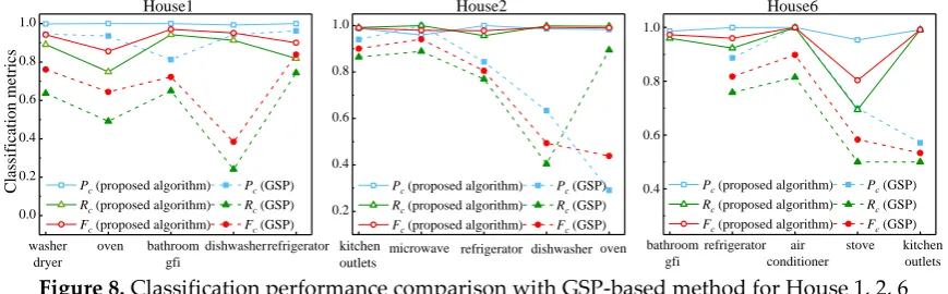
In order to verify the classification accuracy, the results of the proposed algorithm and
498
unsupervised GSP-based approach [29] on house 1, 2 and 6 are represented in Figure.8. It
499
demonstrates that the proposed method provides more accurate classification than GSP-based
500
method for all houses.
501
washer dryer oven bathroom gfi dishwasherrefrigerator 0.0 0.2 0.4 0.6 0.8 1.0Pc (proposed algorithm) Pc (GSP) Rc (proposed algorithm) Rc (GSP)
Fc (proposed algorithm) Fc (GSP)
0.2 0.4 0.6 0.8 1.0 oven dishwasher refrigerator
Pc (proposed algorithm) Pc (GSP)
Rc (proposed algorithm) Rc (GSP)
Fc (proposed algorithm) Fc (GSP) kitchen outlets microwave bathroom gfi refrigerator air conditioner stove kitchen outlets 0.4 0.6 0.8 1.0
Pc (proposed algorithm) Pc (GSP)
Rc (proposed algorithm) Rc (GSP) Fc (proposed algorithm) Fc (GSP)
House1 House2 House6
C la ss if ic at io n m et ri cs
502
Figure 8. Classification performance comparison with GSP-based method for House 1, 2, 6
503
Furthmore, the performance of proposed MFIC algorithm is compared with the state-of-the-art
504
NILM approaches used for low sampling rate and power signals. The MFIC results, FU, are
505
compared with those of the combined k-means/SVM classification [30], FS, the HMM- based method,
506
FH, and the Decision Tree (DT) approach, FDT, as reported in [17]. The results are shown in Table 3.
Table 3 Comparison of four low-rate NILM algorithms using REDD database.
508
Appliance FS FH FDT FU
Air conditioner — 0.12 0.89 99.9
Washer dryer 75.36 0 0.88 94.2
Dishwasher 35.97 0.04 0.32 99.2
Oven 79.13 — — 85.6
refrigerator 94.35 0.90 0.97 97.8 Microwave 25.91 0.47 0.97 97.9
Stove 44.4 0.21 0.33 98.9
House FS FH FDT FU
House 1 77.52 77.06 78.09 92.39
House 2 82.17 82.38 81.41 98.58 House 6 95.58 72.76 75.94 94.53
509
On the one hand, we study the variation of performance with respect to different appliances,
510
mainly including some controllable or high-power loads in REDD database. It can be seen that the
511
MFIC algorithm achieves the best disaggregation in terms of F-measure for all appliances. HMM
512
yields significantly worse results, but it usually performs well identifying refrigerator because the
513
continuity and singleness (i.e., no other devices operates, especially at night) of its operation bring
514
sufficient data for training. The results of k-means/SVM and DT are relatively good but worse than
515
those of MFIC. On the other hand, the average results for three REDD houses are compared. Note
516
that the results of combined k-means/SVM classification and HMM are shown in [30], and the
517
results of DT are reported in [32]. It can be seen that the proposed MFIC algorithm has consistently
518
high performance across all three houses and outperforms other algorithms in both House 1 and
519
House 2. The combined k-means/SVM method shows a higher accuracy for House 6.
520
Moreover, we also use the disaggregation accuracy metric to compare the performance of
521
MFIC algorithm with the Bayesian HMM based technique [21], segmented integer quadratic
522
constraint programming (SIQCP) based algorithm [22], sparse coding (SC), and discriminating
523
sparse coding (discSC) [24].The comparison results are given in Table 4. Obviously, the MFIC
524
algorithm improves significantly compared with the SC-based method from previous work and is
525
slightly superior to the Bayesian HSMM model and SIQCP solver, with the disaggregation accuracy
526
increased by 11.1%, 7.1% respectively.
527
Table 4 Disaggregation accuracy comparison with other methods.
528
Algorithm Disaggregation accuracy (DA)
House1 House2 House6 Mean
MFIC 90.3% 92.0% 95.5% 92.6%
Bayesian HSMM 82.1% 84.8% 77.7% 81.5%
SIQCP 78.4% 86.4% 91.6% 85.5%
SC 57.2% 65.4% 58.1 60.2%
discSC 58.1% 68.3% 53.9% 60.1%
DSC(Greedy) 60.8% 71.1% 61.7% 64.5%
DSC(Exact) 64.3% 74.9% 64.2% 67.8%
5. Conclusion
529
In this paper, a MFIC load disaggregation technique is presented, where the only input is the
530
time-stamped power readings from the smart meter. In order to meet the load monitoring