VLADIMIROV, ANDREY. Modeling Magnetic Field Amplification in Nonlinear Diffusive Shock Acceleration. (Under the direction of Dr. Donald C. Ellison.)
This research was motivated by the recent observations indicating very strong
magnetic fields at some supernova remnant shocks, which suggests in-situ generation of
magnetic turbulence. The dissertation presents a numerical model of collisionless shocks
with strong amplification of stochastic magnetic fields, self-consistently coupled to efficient
shock acceleration of charged particles. Based on a Monte Carlo simulation of particle
transport and acceleration in nonlinear shocks, the model describes magnetic field
ampli-fication using the state-of-the-art analytic models of instabilities in magnetized plasmas
in the presence of non-thermal particle streaming. The results help one understand the
complex nonlinear connections between the thermal plasma, the accelerated particles and
the stochastic magnetic fields in strong collisionless shocks. Also, predictions regarding the
efficiency of particle acceleration and magnetic field amplification, the impact of magnetic
field amplification on the maximum energy of accelerated particles, and the compression
and heating of the thermal plasma by the shocks are presented. Particle distribution
func-tions and turbulence spectra derived with this model can be used to calculate the emission
by
Andrey Vladimirov
A dissertation submitted to the Graduate Faculty of North Carolina State University
in partial fulfillment of the requirements for the Degree of
Doctor of Philosophy
Physics
Raleigh, North Carolina 2009
APPROVED BY:
Dr. James Selgrade Dr. Albert Young
Dr. Donald Ellison Dr. Stephen Reynolds
DEDICATION
This dissertation dedicated to my family. To my mother, whose hard work and
care have made my walk through the early life an easier one. To my father, who, by personal
example, has set the highest standards for me in education and achievement. And to my
treasured wife, whose love, beauty and support has sustained my inspiration and fostered
our happiness. Her patience and understanding in my graduate school years were truly
BIOGRAPHY
I was born in 1982 in the vast and beautiful Eurasian country of Kazakhstan,
which was one of the 15 Soviet Union republics at that time, and now it is an independent
state. By nationality I am Russian, and my native language is Russian.
I earned my B.S. (2002) and M.S. (2004) in physics from St. Petersburg State
Polytechnical University in Russia, where my concentration was physics of space, and I did
my research under Prof. Andrei M. Bykov at the Department of Theoretical Astrophysics
of Ioffe Physical-Technical Institute.
In 2004–2009 I was a graduate student at the Department of Physics of North
Car-olina State University, working on a theoretical research project in the field of astrophysical
ACKNOWLEDGMENTS
I am deeply grateful to my adviser, Prof. Don Ellison, who not only commited
to educating, supervising and directing me in this work, but also was a great source of
encouragement and support throughout my graduate work at NC State University.
This project was carried out in a close collaboration with Prof. Andrei Bykov from
the Ioffe Physical-Technical Institute in Russia. I value very much the priviledge of working
with him and wish to thank him for his participation in this work.
I am also appreciative of the help of the members of the advisory committee, who
agreed to contribute their diverse expertise and time for evaluating this research.
I cannot praise enough many of the NCSU staff members, especially in the
De-partment of Physics and the Office of International Services, who made my graduate school
experience, even in the more complicated situations, stressless and memorable.
Finaly, my heartfelt thanks go to the American and international friends whom I
have met in the past five years in the United States, and whose kindness and hospitality
TABLE OF CONTENTS
LIST OF TABLES . . . vii
LIST OF FIGURES . . . viii
1 Introduction. Interstellar Shocks, Cosmic Rays and Magnetic Fields . . . 1
1.1 Shocks in hydrodynamics . . . 2
1.2 Forward shock of SNRs . . . 3
1.3 The concept of a collisionless shock . . . 6
1.4 Cosmic rays . . . 7
1.5 DSA – test-particle approximation . . . 8
1.6 DSA – nonlinear regime . . . 14
1.7 Magnetic field amplification in shocks . . . 16
1.8 Turbulence . . . 18
2 The Problem of Nonlinear DSA. . . 20
2.1 Analytic models . . . 21
2.2 Particle-in-cell (PIC) codes . . . 23
2.3 Monte Carlo Simulation . . . 26
2.4 Objectives of this dissertation . . . 27
3 Model . . . 29
3.1 Core Monte Carlo . . . 30
3.1.1 Overview . . . 30
3.1.2 Particle propagation, pitch angle scattering . . . 33
3.1.3 Motion of the scattering medium . . . 37
3.1.4 Calculating particle distribution and its moments . . . 42
3.1.5 Introducing particles into the simulation . . . 46
3.1.6 Test particle case of DSA . . . 50
3.1.7 Shock compression ratio in nonlinear DSA . . . 55
3.1.8 Nonlinear structure of the shock precursor . . . 63
3.1.9 Summary . . . 67
3.2 Magnetic Field Amplification . . . 68
3.2.1 Resonant cosmic ray streaming instability . . . 70
3.2.2 Bell’s nonresonant instability . . . 72
3.2.3 Nonresonant long-wavelength instability . . . 73
3.2.4 Evolution of turbulence in a nonlinear shock – other effects . . . 74
3.2.5 Generalized model of magnetic turbulence amplification . . . 81
3.2.6 Analytic solutions for turbulence spectrum . . . 83
3.2.8 Tests of the numerical integrator . . . 96
3.2.9 Turbulence and equations of motion . . . 98
3.3 Particle transport . . . 105
3.3.1 Bohm diffusion limit . . . 105
3.3.2 Resonant scattering by Alfv´en waves . . . 106
3.3.3 Diffusion in short scale turbulent fluctuations . . . 106
3.3.4 Low energy particle trapping by turbulent vortices . . . 107
3.3.5 Implementation of diffusion models in the Monte Carlo code . . . . 109
3.4 Parallel computing with MPI . . . 113
4 Applications of the model. . . 116
4.1 Turbulence growth rate and self-consistent solutions . . . 117
4.1.1 Model . . . 117
4.1.2 Results . . . 118
4.1.3 Discussion . . . 130
4.2 Impact of MFA on the maximum particle energy . . . 132
4.2.1 Model . . . 132
4.2.2 Results . . . 133
4.2.3 Discussion . . . 134
4.3 Turbulence dissipation in shock precursor . . . 138
4.3.1 Model . . . 138
4.3.2 Results . . . 139
4.3.3 Discussion . . . 153
4.4 Bell’s nonresonant instability and cascading in nonlinear model . . . 154
4.4.1 Model . . . 154
4.4.2 Results . . . 156
4.4.3 Discussion . . . 160
4.5 Fits for the nonlinear shock structure . . . 162
4.5.1 Model . . . 162
4.5.2 Results . . . 162
4.5.3 Discussion . . . 163
4.6 Spectrum and angular distribution of escaping particles . . . 168
4.6.1 Model . . . 168
4.6.2 Results . . . 169
4.6.3 Discussion . . . 170
5 Conclusions. . . 171
REFERENCES . . . 174
APPENDICES . . . 187
A. Numerical integrator for model with isotropization . . . 188
LIST OF TABLES
Table 3.1 Test of iterative search of the compression ratio,rtot. . . 60
Table 3.2 Test of performance boost with parallel computing. . . 115
Table 4.1 Summary of Non-linear Simulation in a Cold ISM . . . 144
Table 4.2 Summary of Non-linear Simulation in a Hot ISM . . . 144
Table 4.3 Self-consistent shock parameters forαH = 0.0. . . 165
Table 4.4 Self-consistent shock parameters forαH = 0.5. . . 166
LIST OF FIGURES
Figure 1.1 Tap water in a sink forms a shock. . . 2
Figure 1.2 Schematic structure of an SNR. . . 4
Figure 1.3 The youngest known galactic SNR, G 1.9+0.3. . . 5
Figure 1.4 The all particle spectrum of cosmic rays. . . 9
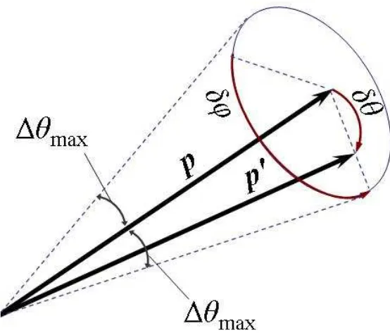
Figure 3.1 Pitch angle scattering diagram. . . 34
Figure 3.2 Particle trajectories calculated in the Monte Carlo code. . . 36
Figure 3.3 Particle diffusion in the Monte Carlo code. . . 36
Figure 3.4 Advection with diffusion. . . 39
Figure 3.5 Particle heating in a compressing flow. . . 41
Figure 3.6 Generation and detection of thermal particle population. . . 47
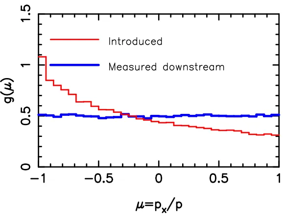
Figure 3.7 Relaxation of particle distribution to isotropy. . . 51
Figure 3.8 Test of introduced particle distribution isotropy.. . . 51
Figure 3.9 Test particle case of DSA.. . . 52
Figure 3.10 Particle trajectories in DSA. . . 54
Figure 3.11 Iterative estimation of compression ratio.. . . 61
Figure 3.12 Momentum and energy conservation illustration. . . 62
Figure 3.13 Search for the self-consistent compression ratio. . . 65
Figure 3.14 Precursor smoothing for momentum and energy conservation. . . 66
Figure 3.15 Effect of flow compression on turbulence spectrum. . . 99
Figure 3.16 Amplification of turbulence spectrum. . . 99
Figure 3.18 Cascading of seed power law spectrum of turbulence. . . 100
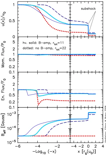
Figure 4.1 Shock structure with and without MFA . . . 120
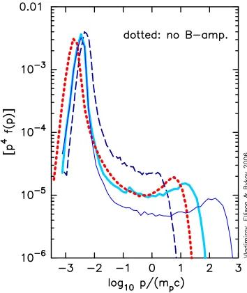
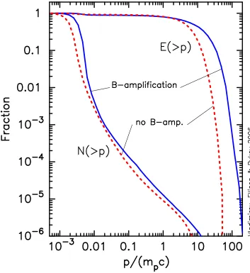
Figure 4.2 Phase space distributions with and without MFA . . . 121
Figure 4.3 Turbulence and particle spectra with MFA . . . 123
Figure 4.4 Acceleration efficiency with and without MFA. . . 124
Figure 4.5 Comparison of shocks with different far upstream fieldsB0. . . 126
Figure 4.6 Shocks with varying falf . . . 127
Figure 4.7 Distribution functions for the shocks shown in Figure 4.6. . . 129
Figure 4.8 Flow structure: unmodified versus nonlinear. . . 135
Figure 4.9 Proton spectra and acceleration times: unmodified versus nonlinear.. . . 136
Figure 4.10 Dissipation effects in unmodified shocks . . . 140
Figure 4.11 Dissipation effects in nonlinear shocks . . . 141
Figure 4.12 Nonlinear shocks with dissipation, cold ISM . . . 147
Figure 4.13 Nonlinear shocks with dissipation, hot ISM. . . 148
Figure 4.14 Particle distribution with dissipation, cold ISM. . . 149
Figure 4.15 Particle distribution with dissipation, hot ISM . . . 150
Figure 4.16 Enlarged subshock region in the hot ISM case. . . 152
Figure 4.17 Shocks with turbulence generation by Bell’s nonresonant instability . . . 156
Figure 4.18 Spectral properties of shocks shown in Figure 4.17 . . . 157
Figure 4.19 Turbulence spectrum at different spatial locations. . . 158
Figure 4.20 Angular distribution of escaping particles . . . 169
Chapter 1
Introduction. Interstellar Shocks,
Cosmic Rays and Magnetic Fields
What happens after a massive star explodes at the end of its life cycle as a
su-pernova (SN)? Why are the rims of susu-pernova remnants (SNRs) so thin and luminous in
the radio, X-ray and gamma ray spectral ranges? Where and how are cosmic rays (CRs)
produced? What does it take to explain the dynamics of matter in the most energetic
sys-tems in space, including the cosmological large scale structure of the Universe? The current
state of affairs in astrophysics makes it clear that, in order to answer these questions, the
phenomenon of shocks must be studied in detail. The low gas densities in many cosmic
environments make the shocks collisionless (see Section 1.3), which gives them properties
different from those of the collisional terrestrial shocks.
Understanding shocks is as important for astrophysicists as describing
electromag-netic waves is for radio engineers. Shocks are born whenever gases or fluids are forced to
move at a supersonic speed. They compress and heat the interstellar matter (ISM),
trans-fer energy and momentum, produce cosmic rays that fill and affect the Universe, and, as
recent observations show, shocks may produce and strongly amplify turbulent magnetic
fields. Electromagnetic radiation from processes in shocks is a powerful diagnostic of the
1.1
Shocks in hydrodynamics
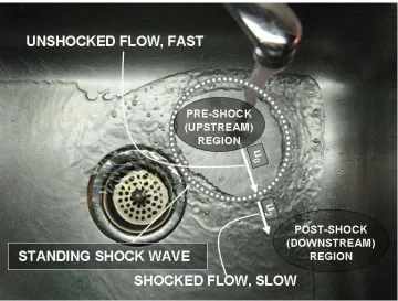
I would like to illustrate shocks with a phenomenon that we encounter on a daily
basis – a standing shell shock in a kitchen sink formed by the quickly running water from
the tap.
Figure 1.1: Tap water in a sink forms a shock.
As seen in Figure 1.1, the falling water hits the bottom of the sink and moves
outward at a speed that exceeds the speed of the surface waves in water of the local depth.
This makes a shock form, a relatively stationary enclosed boundary, at which the speed
of the water flow abruptly drops, and the depth increases. The direction in of the shock’s
apparent motion depends on the choice of the observer’s reference frame, but let us adopt a
convention that unambiguously determines thedirection of shock propagation. I will define
media moves with respect to the unshocked medium. In the case of the shock in a sink, the
unperturbed medium is inside of the circular shell, and it moves outward. Therefore, the
shock is directed inward (i.e., any small arc of the shock boundary is moving towards the
center with respect to the water inside the boundary). The arrows show the velocity of the
water with respect to the shock.
A similar inward-directed shock exists in the Solar System: the Solar wind,
com-posed of fast charged particles emitted by the Sun, moves radially outward and collides with
the cold interstellar material approximately 80-100 AU from the Sun (an astronomical unit,
1 AU≈1.5·1011 cm, is close to the distance between the Sun and the Earth). The so-called termination shock forms there. At this thin boundary, the Solar wind becomes compressed
and heated, and its speed drops by a factor of 2-5. Both Voyager spacecrafts recently passed
through the termination shock on their way out of the Solar System [114, 24, 113, 23].
1.2
Forward shock of SNRs
After a star with an initial mass greater than approximately 8M(M ≈2·1033g
is the mass of the Sun) runs out of its fusion fuel, or a white dwarf accreting mass from
another star in a binary system reaches the critical mass and ignites, an explosion will
occur. This explosion, powered either by gravity, or by thermonuclear fusion, is known as
a supernova, and ejecting up to 1051 ergs in kinetic energy, it can be bright enough to see
with the naked eye thousands of light years away. A remnant of a supernova in our Galaxy
may remain visible to radio, optical and X-ray telescopes for hundreds or thousands of years
after the explosion, as it expands into the interstellar medium, cools and gradually fades.
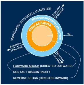
Hydrodynamic simulations and observations show a common structure of flow that
forms in SNRs, as shown in Figure 1.2. The metal-rich material (ejecta) is thrown out from
the star at speeds of several thousand kilometers per second. It ploughs through the
low-density ISM, and eventually forms a strong forward shock in front of it, directed outward.
A contact discontinuity separates the metal-rich ejecta material from the low-metallicity
shocked ISM. Simulations show that a reverse shock, may form in the ejecta. While the
inverse shock is directed inward (i.e., it shocks the material coming from the interior of
the reverse shock boundary), it may be physically moving outward or inward at different
Figure 1.2: Schematic structure of an SNR.
velocities of the unshocked medium with respect to the forward and the reverse shocks. The
dotted lines indicate the expansion of the forward shock in time.
Of particular importance to us is the forward shock, because it can be very strong,
sonic Mach number reaching the values of several hundred. There are two important
differ-ences between the shell shocks in Figure 1.1 and Figure 1.2. First, the shock in the sink is
directed inward (it sweeps up water coming from the interior of the circle), while the SNR
forward shock is directed outward (sweeping up the interstellar matter outside of it). The
second difference is that the sink shock is stationary, i. e., its radius remains constant in
time, but the SNR expands into a stationary unshocked ISM, increasing the radius of the
forward shock.
Figure 1.3: The youngest known galactic SNR, G 1.9+0.3.
as the youngest known supernova remnant in the Galaxy. It was very recently identified
as one by an international team led by NCSU astronomers [102] and [67]. It provides an
illustration of a typical spatially resolved SNR imaged in X-rays. In Figure 1.3 (image
credit: Prof. S. Reynolds, NCSU, [102]), the dotted line maps the approximate location of
the forward shock1, the dotted arrows indicate the direction of the shock movement with respect to the interstellar medium, and the solid arrows indicate the directions and the
relative magnitudes of the velocities of the unshocked (the long arrow) and the shocked
(the short arrow) plasma, with respect to the shock. Note that in the following text we
usually adopt the reference frame in which the shock is at rest, and the plasma is flowing
1
into the shock at a supersonic speed. This approach corresponds to the flow directions
shown in Figures 1.1 and 1.3.
1.3
The concept of a collisionless shock
Generally, gas flowing into a shock gets compressed and heated in a narrow region.
But how narrow can this region be for a shock in an astrophysical plasma? In order to change
the density, bulk speed and temperature, the gas particles must experience a few strong
collisions, and the thickness of the shock can therefore be estimated as the mean free path
of particles between collisions. Indeed, for shocks in dense gases (for example, air) a particle
mean free path is comparable to the shock thickness. However, in an attempt to apply the
same reasoning to interstellar or interplanetary shocks, one runs into a complication.
For a plasma consisting of fully ionized hydrogen, the cross section of Coulomb
collisions between protons is formally infinite [110], but we can roughly estimate the cross
section of collisions that are strong enough to change the energy of the particles significantly.
If by ’significantly’ one means that the change energy due to collision must be comparable
to the thermal energy, then the protons must approach each other within a distancercsuch that
e2 rc
=kBT. (1.1)
Here and in the rest of the equations in this dissertation, the CGS system of units is
adopted. The quantityeis the elementary charge, and the left-hand side of Equation (1.1) is the electrostatic potential energy of two protons separated by the distancerc. The right-hand side is the characteristic thermal energy of protons in a gas of temperatureT (kB is the Boltzmann constant). This gives a rough estimate of the collision cross section
σ =πrc2= πe
4
kB2T2 (1.2)
and of the mean free path
Λ = 1
σn = k2
BT2
πe4n, (1.3)
which means that shocks just do not have room to form in the Solar wind near the Earth.
However, spacecraft observations clearly indicate numerous interplanetary shocks of various
strengths traversing the Solar System. Measurements reveal that the interplanetary shocks
are much thinner then the number above: observed thicknesses are around Λ∼107−1010cm
[107].
These observational data are successfully explained by the theory of collisionless
shocks, which assumes that in the transition region of the shock, particles collide not with
each other, but with inhomogeneities of magnetic fields. This shrinks the thickness of the
transition region down to the scales of (multiple) proton gyroradii (see Section 6.4 of [81]). A
shock in which collisions between particles play a negligible role compared to the dynamics
of the particles in stochastic magnetic fields is called a collisionless shock, and the term
collisionless plasma is widely used to define the systems in which similar conditions exist.
An interesting property of collisionless plasmas is that, due to the absence of
particle-particle collisions, the time scales of thermalization of non-equilibrium energy
dis-tributions of particles are extremely large. This allows for the existence and sustainability
of a superthermal component in the particle distribution (i.e., energetic particles). Present
research, along with other models, shows that the superthermal particles may be not just a
minor admixture to the thermal particle pool, but, on the contrary, they may dominate the
dynamics of a collisionless shock. This assertion is explained in the following two sections.
1.4
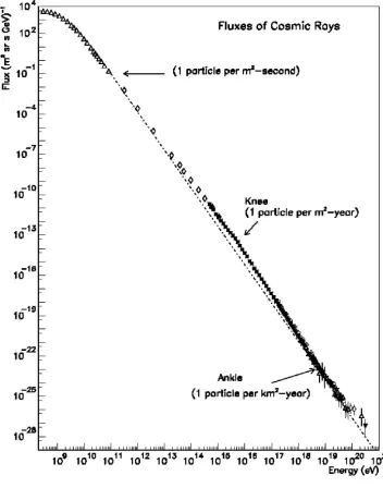
Cosmic rays
Cosmic rays (CRs) are charged particles, first seen as radiation coming from space
in a balloon experiment performed by Victor Hess in 1912, and identified as charged nuclei by
Phyllis Freier and others in 1948 [57]. The spectrum of these particles spans many decades
in particle energy (107 to 1020 eV (!) per nucleus) as well as in flux (from 1 cm−2s−1sr−1
for energies of 1 GeV and above, down to 1 particle per square kilometer per century for
energies over 1020 eV [34]).
From the multitude of observational data on CRs, it is known that the lower energy
CRs come from the Sun, and the higher energy CRs (over 1-10 GeV) are of Galactic origin.
CRs are therefore the second most important source of information about deep space after
compo-sition, temporal variation and directional distribution of CRs is extensive and longstanding.
It requires answering two major questions: how CRs are produced, and what happens to
them en route from the source to the detector on Earth.
The spectrum shown in Figure 1.4 (image credit: S. Swordy, University of Chicago,
[116]) is a compilation of the various measurements. This spectrum cannot be identified
with a single CR source or even multiple CR sources; in fact, it represents a superposition
of the multitude of Galactic CR sources, integrated over a time scale of millions of years,
and convolved with the history of their propagation in the Galactic magnetic fields from all
parts of the Galaxy.
Most researchers these days are convinced that the bulk of the Galactic CRs at
least up to the ‘knee’ of the CR spectrum (i.e., up to the energies of 3·1015eV), are produced
in astrophysical collisionless shocks [19]. While the details of this process may be uncertain
(how much shocks of individual SNRs contribute to the CR production, in comparison with
SNR shock ensembles in the so-called superbubbles, how the interstellar dust is involved,
etc.), the general idea is commonly accepted now.
The process that accelerates the particles to ultra-relativistic energies in shocks is
known as the first order Fermi process2, or diffusive shock acceleration (DSA).
1.5
DSA – test-particle approximation
Diffusive shock acceleration, DSA, also known as the first order Fermi process
(often abbreviated as Fermi-I) was first applied to the problem of cosmic ray production in
shocks by several independent groups and researchers at the end of the 1970s [9, 20, 79, 40].
The best simple mechanical analogy to this process is the acceleration of a rubber ball
elastically bouncing back and forth between two massive walls, as the walls are slowly
moved towards each other. In a shock, the role of the moving walls is played by the bulk
gas flow: the faster-moving unshocked gas and the slower moving shocked gas form an
effectively converging system.
The spectrum of particles accelerated in such a manner may be calculated in
various ways, including a kinetic approach (see, e.g., [79]). Consider a one-dimensional
2
shocked flow, with the shock located atx= 0, and the flow speed
u(x) =
u0, x <0, u2, x >0,
(1.4)
whereu0 is the upstream and u2 < u0 – the downstream speed, and let there be a minor
admixture of energetic particles that move diffusively in the bulk plasma, the diffusion
being isotropic in the plasma frame. Assume that the diffusion coefficient is independent of
momentum and of coordinate (except it may have different constant values upstream and
downstream of the shock):
D(x) =
D0, x <0, D2, x >0,
(1.5)
In a steady state, diffusive propagation of the energetic particles, as they are being advected
downstream by the flow, can be described by the equation
u(x)∂f(x, p)
∂x =D(x)
∂2f(x, p)
∂2x , (1.6)
wheref(x, p) is the particle distribution function, such that f(x, p)dxdydzdpxdpydpz is the number of particles in the phase space volumedxdydzdpxdpydpz, and that f(x, p) does not depend on the direction ofp. Suppose the incoming energetic particles have a distribution
function:
lim
x→−∞f(x, p) =f0(p)≡f0
1
p20δD(p−p0), (1.7)
wherep0 is a momentum such that the corresponding particle speed is much greater than u0, p is the current particle momentum, and δD is the Dirac delta-function. Assume the trivial downstream boundary condition
lim
x→+∞f(x, p)<∞, (1.8)
and define the conditions at the discontinuity pointx= 0:
lim
x→0−f(x, p) = xlim→0+f(x, p), (1.9)
lim x→0−
−D0
∂f(x, p)
∂x −
p
3
∂f(x, p)
∂p
= lim
x→0+
−D2
∂f(x, p)
∂x −
p
3
∂f(x, p)
∂p
The first equation expresses the requirement of continuity of the particle density, and the
second – of particle flux. The general solution of equation (1.6) may be written as
f(x, p) =
A(p) exp
u0x D0
+B(p), x <0
C(p) exp
u2x D2
+E(p), x >0.
(1.11)
Substitution of this form into the boundary condition (1.7) results in
B(p) =f0(p), (1.12)
and using the boundary condition (1.8) gives
C(p) = 0. (1.13)
Now we can use the conditions at x = 0, where the density continuity equation (1.9) can help constrainA(p) andE(p) in (1.11):
A(p) +f0(p) =E(p), (1.14)
and flux continuity condition (1.10), rewritten as
D0 lim
x→0−
∂f(x, p)
∂x
−D2 lim
x→0+
∂f(x, p)
∂x
=−p 3
∂f(0, p)
∂p
, (1.15)
gives
−D0A(p) u1 D0
exp (0)−0 =−p 3
dE(p)
dp (u0−u2). (1.16)
Combining (1.14) and (1.16), we get
p
3
dE(p)
dp (u0−u2) +E(p)u1 =u1 f0 p2 0
δD(p−p0), (1.17)
which can easily be integrated, assumingE(0) = 0, and the solution is
E(p) =E0
p0 p
s
H(p−p0), (1.18)
where
E0 =
3N0u0
p30(u0−u2) (1.19)
s = 3u0
u0−u2
andH(z) is the Heaviside step function:
H(z) =
0, x <0
1, x≥0. (1.21)
Finally, the solution of equation (1.6) with boundary conditions (1.7), (1.8) and the
conti-nuity conditions at the shock (1.9) and (1.9) is:
f(p) =
E0 p0 p s
H(p−p0)eu0x/D0+ f0
p20δD(p−p0)
1−eu0x/D0
, x <0,
E0
p0 p
s
H(p−p0), x >0.
(1.22)
This is the so-called test-particle solution of the problem of diffusive shock acceleration,
meaning that the accelerated energetic particles are implicitly assumed to be a small
ad-mixture in the vast thermal pool. This assumption is likely to fail for strong collisionless
shocks, leading to serious modifications of the solution, on which the present work
concen-trates.
Let us analyze the basic properties of the test-particle solution (1.22).
• It requires that some seed particles be introduced, represented by f0(p), but in real
shocks these seed particles must be produced from the thermal pool (injected, as the
theorists of the particle acceleration field prefer to put it). This model is unable to
predict anything about the injection of particles, and their numberf0and momentum p0 are free parameters of the test-particle model.
• Once the seed particles are introduced, they form a power-law superthermal tail up-ward of the injection momentum p0, with the indexs that depends only on the
pre-shock and the post-pre-shock speed, as given by equation 1.20. That equation can be
re-written in terms of the shock compression ratio r=u0/u2 as
s= 3u0
u0−u2 =
3r
r−1. (1.23)
For the strongest hydrodynamic shocks in a non-relativistic monatomic gas, the
com-pression ratio r = u0/u2 approaches the value of r = 4 (this well known result can
easily be derived from the Hugoniot adiabat presented in Section 3.1.7 in the limit
index of the accelerated particle distributions= 4. A particle distributionf(p)∝p−4
extending to p → ∞ in unphysical, because the internal energy of such distribution diverges logarithmically at p → ∞. This means that, if compression ratios ofr = 4 or greater3 are achieved in space, there must be some process responsible for limiting
the maximum achievable energy. The escape of the highest energy particles from the
system, or a finite time of particle acceleration in a time-dependent calculation may
determine the high-energy cutoff of the particle spectrum. Such processes are not
included in this simplistic model.
• The basic physical assumption that leads to the emergence of the power-law superther-mal tail of f(p) is that the particles are subject to diffusion isotropic in the plasma frame (this is expressed by the equation (1.6)). This implies that we are dealing with
a collisionless shock (otherwise the superthermal particles would have to
thermal-ize through collisions with their thermal counterparts) that has a certain stochastic
magnetic field structure (i.e., turbulence), responsible for particle scattering. The
properties of these stochastic fields are, obviously, beyond the scope of this model,
but they must influence the solution by at least determining the diffusion coefficient
D(x, p). In fact, as will be shown later, the magnetic turbulence that confines the particles to the acceleration site, and allows for the Fermi-I acceleration, is probably
produced by the accelerated particles themselves, which raises the question of solving
the particle acceleration problem consistently with the turbulence production process.
It turns out that all of these properties of the test-particle make it unable to explain some
observations of interstellar collisionless shocks (see the next section), which calls for a better
model.
3
1.6
DSA – nonlinear regime
The example from classical mechanics that illustrates the first order Fermi process
– the rubber ball bouncing between two converging walls – may also be used to understand
the nonlinear aspects of diffusive shock acceleration. The ball in classical mechanics gains
energy at every collision, but only as long as the walls are much heavier than the ball and
continue to move inward despite the ball’s kicks. But what if the ball gains enough energy,
so the recoil of the walls makes them slow down their convergence? In this case we would
have to account for the feedback of the ball on the walls. This makes the problem nonlinear.
Suppose, we put one ball between the walls, and its kinetic energy after N cycles becomes
K. If we were to put not one, but two balls, the their total energy afterN cycles would be less than 2K, because the recoil of the two balls would have slowed the walls down more efficiently than the recoil of one ball. Similarly, in shock acceleration, the energy of the bulk
plasma flow powers the energetic particle acceleration, but once the accelerated particles
gain enough energy to push back on the flow, the situation changes dramatically. Such a
system is called anonlinear, or a multicomponent shock wave, and is the subject of study
of nonlinear diffusive shock acceleration theory.
There is a number of reasons to believe that strong shocks in space accelerate
particles very efficiently, thus operating in the nonlinear regime. I outline these reasons
below, and some of them will be elaborated on further in the dissertation.
1. Energy considerations. The energy density of Galactic cosmic rays at the location of
the Solar System is ε ≈0.6 eV·cm−3, and their characteristic age inferred from the
radioactive nuclei in CRs is of order τcr ≈107 yr. Assuming that the escape of CRs
from the Galaxy has the time scale τcr and that the escape is balanced by the CR
production one can estimate the required power of CR production in the Galaxy as
Pcr= εV
τcr = 3·10
41erg s−1,
whereV is the volume of the Galaxy,V =π(105pc)2·100 pc = 3·1012pc3≈1068cm3. Assuming that all of these cosmic rays are produced by shocks of SNRs, which occur
once in τsn = 100 yrs and release E = 1051 erg as the kinetic energy of the shock
wave, the Galactic energy production in the form of shocks is
Psk= E τsn
Our estimates of the quantities Pcr and Psk are comparable, which means that SN
shocks may easily be required to have an efficiency on the order of tens of percent of
converting the bulk motion energy into the energy of accelerated particles. See also
[19] for a detailed discussion.
2. Numerical simulations (e.g., [43, 89, 74, 22]) predict efficient particle acceleration given
the simplest physically realistic model of particle injection, thermal leakage. The above
mentioned models use different techniques, but all of them predict that in a strong
collisionless shock, the energy density of energetic particles becomes comparable to
the kinetic energy density of the flow, thus making the problem nonlinear.
3. Analysis of the morphology of resolved SNRs indicates high compression ratios at the
forward shock (e.g., [125, 33]) which is consistent with the predictions of nonlinear
particle acceleration theories. There is also observational evidence of the nonlinearity
of DSA that comes from the analysis of nonthermal emission spectra (e.g., [103, 2])
and from spacecraft observations of the Earth’s bow shock (e.g., [51]).
4. Recent observations indicate that magnetic fields in some SNR shocks are much
stronger than the ambient magnetic fields, which makes many researchers believe
that magnetic fields are amplified in situ, i.e. in the shocks, by the shock-accelerated
particles. If that is the case, the energy density of the accelerated particles must be
no less than the energy density of the amplified magnetic fields, and, according to the
observational estimates, the latter is a significant fraction of the dynamical pressure
of the shock flow. This necessitates the nonlinear DSA (see, e.g., [53]).
The nonlinear DSA theory was developed by various researchers in the 1980s.
Although the details of the models may differ, all of them agree on the following: when
the energetic particles gain enough energy to feed back on the flow, the unshocked plasma
slows down and becomes compressed even before it reaches the viscous shock (the latter
is renamed a subshock in context of nonlinear DSA), which means that a shock precursor
forms in the upstream region (x <0); the maximum particle energy must be limited either by the age, or by the size of the shock, and if particles of the highest energies are allowed
1.7
Magnetic field amplification in shocks
Recent observations and modeling of several young supernova remnants (SNRs)
suggest the presence of magnetic fields at the forward shock (i.e., the outer blast wave) well
in excess of what is expected from simple compression of the ambient circumstellar field,
Bism. These large fields are inferred from:
• spectral curvature in radio emission (e.g., [103, 13]) ,
• broad-band fits of synchrotron emission between radio and non-thermal X-rays (e.g., [14, 124], see also [35]),
• sharp X-ray edges (e.g., [121, 6, 124, 45, 32]), and
• rapid variability of nonthermal X-ray emission from bright filaments in SNRs (first reported by [119]).
While these methods are all indirect, fields greater than 500µG are inferred in the supernova remnant Cassiopeia A and values of at least several 100µG are estimated in Tycho, Kepler, SN1006, and G347.3-0.5. If Bism ∼ 3−10 µG, amplification factors of 100 or more may
be required to explain the fields immediately behind the forward shocks and this is likely
the result of a nonlinear amplification process associated with the efficient acceleration
of cosmic-ray ions via diffusive shock acceleration (DSA). The magnetic field strength is
a critical parameter in DSA and also strongly influences the synchrotron emission from
shock accelerated electrons. Since shocks are expected to accelerate particles in diverse
astrophysical environments and synchrotron emission is often an important emission process
(e.g., radio jets), quantifying the magnetic field amplification has become an important
problem in particle astrophysics and has relevance beyond cosmic-ray production in SNRs.
These highly amplified magnetic fields are most likely an intrinsic part of efficient
particle acceleration by shocks. This strong turbulence, which may result from cosmic ray
driven instabilities, both resonant and non-resonant, in the shock precursor, is certain to
play a critical role in self-consistent, nonlinear models of strong, cosmic ray modified shocks.
Although plasma wave instabilities in presence of accelerated particles have been studied in
the context of shock acceleration before (e.g., [9, 82]), it was only recently suggested that
∆B B0 [11]. Since then, new models of plasma instabilities possibly responsible for
efficient magnetic field amplification were proposed [86, 10, 30] and studied in context of
shock acceleration [99, 3, 122, 129].
All these plasma instabilities are assumed to amplify pre-existing waves in a plasma
in the presence of an underlying uniform magnetic fieldB0 parallel to the flow4. The two
models of interest that will be applied to the present work are:
1. Resonant CR streaming instability (see [106, 82] and [11, 3, 122]), in which particles
of a certain momentum amplify Alfv´en waves with a wavenumber equal to the inverse
gyroradius of the particle, and
2. Nonresonant CR streaming instability of short-wavelength modes (suggested by [10]),
which I will sometimes refer to as Bell’s instability, in which the diffusive electric
current of CRs amplifies almost purely growing waves with wavenumbers much greater
than the inverse particle gyroradius.
I should also mention a nonresonant instability that produces long-wavelengths modes and
may also be important in shocks (see [30] and Section 3.2.3), which I am planning to apply
to the modeling of shocks in the future, as well as other possible mechanisms (e.g., [91]).
Amplification of magnetic turbulence has great importance in the process of DSA.
The amplified turbulence provides the stochastic magnetic fields that scatter the
acceler-ated particles, allowing them to participate in the Fermi-I process. The properties of the
particle scattering are therefore dependent on the spectrum of stochastic magnetic fields,
yet the latter are produced by the accelerated particles. This complex connection between
particles and waves in shocks adds to the nonlinear nature of shock acceleration, discussed
in Chapter 2. Therefore, magnetic field amplification affects the observable nonthermal
synchrotron emission from shocks in two ways: it determines the structure and strength of
the magnetic fields in which the emission occurs, and shapes the spectrum of the radiating
energetic particles.
4
1.8
Turbulence
Studying strong magnetic field amplification in interstellar shocks inevitably makes
us face the subject of magnetohydrodynamic (MHD) turbulence. Usually turbulence is
defined as chaotic fluid motion, that is, a motion with a very sensitive dependence on initial
conditions. Chaotic behavior makes turbulent motions effectively non-deterministic, but
they can be studied using statistical methods.
Motions of gases and fluids of high Reynolds number tend to transit to the
tur-bulent regime (see, e.g., [83, 96]), which is encountered on a regular basis in areas ranging
from plasma fusion engineering and race car design to air transport, plumbing, golf and
food processing (e.g., [58, 115, 18, 112]). Driven by the need of applications like
meteo-rology, climate modeling, aerospace engineering, and others, turbulence research has been
conducted for many decades, and is a challenging field of mathematics and physics (e.g.,
[56]). Conducting fluids (plasmas) easily develop and sustain magnetic fields, and the MHD
turbulence regime, occurring in plasmas, is even more complicated by the magnetic field
interactions than its hydrodynamic counterpart [17].
Considering that plasmas constitute a large fraction of all baryonic matter in
space, their properties have pervading importance for astrophysics. Namely, turbulence
in plasmas determines cosmic ray acceleration and propagation, plays a crucial role for
angular momentum transfer in accreting systems and impacts the properties of gravitational
collapse. The list of astrophysical objects affected by MHD turbulence is therefore extensive:
large scale structure of the Universe, quasars, accreting binary systems, forming stars,
supernova remnants, etc.
The primary sources of information about MHD turbulence are spacecraft
obser-vations of interplanetary space and numerical simulations. The former provide real, but
often hard to interpret data, the bottom line of which is that turbulence often consists of
stochastic perturbations of plasma velocities and magnetic fields spanning many decades
of the spatial scales. Oftentimes, the Fourier spectrum of spatial structure of turbulent
fluctuations reveals a power-law distribution of energy in wavenumber space. The
numeri-cal simulations have the advantage of providing data that is easy to analyze and snumeri-cale for
practically applicable theories.
three dominant processes: energy supply, spectral transfer of energy and dissipation.
Con-sider a fluid flow in a pipe, where a large flux of the fluid leads to the development of a
hydrodynamic instability that creates vortices (eddies) breaking the laminar flow. In this
way energy is supplied to the turbulence in the form of large-scale vortices. These eddies
then break down into smaller eddies – this way, spectral energy transfer (cascade) from
large to small scales is realized. As the scale of the turbulent structures due to cascading
becomes smaller, fluid viscosity plays an increasingly greater role, eventually leading to the
dissipation of the smallest eddies into heat.
The MHD turbulence, as mentioned above, is difficult to describe. It was originally
treated and analyzed as a set of small perturbations (i.e., plasma waves) moving in the
large-scale uniform magnetic field and weakly interacting with each other (the so-called
Iroshnikov-Kraichnan approach [70, 78]). However, Goldreich and Sridhar [64]5 point out
that this approach may be inappropriate for MHD turbulence due to its inherent anisotropy
introduced by the magnetic field [55]. The bottom line of their theory and of the subsequent
simulations of MHD is that the magnetic field plays a stabilizing role. The cascading takes
place mostly for wave vectors perpendicular to the uniform magnetic field, while the parallel
cascade is suppressed.
A comprehensive source on classical theory of hydrodynamical turbulence is [96].
Modern advances in the study of MHD turbulence is presented in [17].
5
Chapter 2
The Problem of Nonlinear DSA
The general problem of nonlinear diffusive shock acceleration of charged particles
(DSA) can be formulated as follows: given a supersonic flow with a speed u0 of a plasma
with a number densityn0, temperatureT0 and a pre-existing magnetic fieldB0, and given
the location x = 0 where this flow develops a subshock, find the distribution of particles
f(x,p, t) and electromagnetic fields in the shock vicinity. This problem is complicated by two facts: a) particle acceleration occurs due to complex motions of particles in the
turbulent magnetic field, but the magnetic turbulence itself is dependent upon the motion
of the accelerated particles, and, b) if particle acceleration is efficient, different parts of the
particle spectrum interact with each other (i.e., the accelerated particles push back on and
slow down the flow of the thermal particles).
This problem cannot be practically tackled by particle simulations from first
prin-ciples like Maxwell’s equations and Lorentz force (see Section 2.2), and the most
computa-tionally expensive operations must be performed analytically. Namely, all currently existing
models of nonlinear DSA, including the one discussed in this dissertation, assume that the
accelerated particles propagate diffusively with some diffusion coefficient, or mean free path,
prescription. This allows the models to eliminate the need to describe the complex
inter-actions between particles and waves, and to concentrate on the physical aspects of particle
2.1
Analytic models
In successful analytic models, a one-dimensional steady state shock with a
non-linear precursor is described by the flow speedu(x, t), mass density of the plasma ρ(x, t) and an isotropic distribution function of energetic particles, fcr(x, p, t). The above
men-tioned macroscopic quantities must be consistent with the fundamental conservation laws:
mass, momentum and energy must be conserved. These conditions are expressed with the
following system of equations:
ρu = const, (2.1)
ρu2+Pth+Pcr+Pmag = const, (2.2)
1 2ρu
3+ γth γth−1
Pthu+ γcr γcr−1
Pcru+
3
2Pmagu+Qesc = const. (2.3) and the evolution of the particle distribution is governed by the kinetic equation of CR
transport
∂ ∂x
D(x, p) ∂
∂xf(x, p)
−u∂f(x, p)
∂x + 1 3 du dx
p∂f(x, p)
∂p +Qinj= 0. (2.4)
Equations (2.1), (2.2) and (2.3) represent conservation of mass, momentum and energy
fluxes, respectively. Equation (2.4) is the kinetic equation describing propagation of
cos-mic rays in the diffusion approximation. The expressions above are, essentially, a direct
generalization of the test particle model of shock acceleration demonstrated in Section 1.5,
complemented by the treatment of the flow speed u(x) variability upstream. Let us use the following notation for the flow speed and other quantities at points of interest: u0 is
the far upstream flow speed, u2 is the downstream flow speed, and u1 is the flow speed
just before the subshock. Thus, in the upstream region, x <0, the flow speed varies from
u(x = −∞) = u0 to u(x = −0) = u1 < u0, and then jumps in a viscous subshock to
u(x= +0) = u2 < u1. Let us also define the total compression ratio, rtot =u0/u2 and the
subshock compression ratiorsub=u1/u2.
To close the model, one must describe the evolution of thermal gas pressure, Pth,
define the cosmic ray pressure, Pcr and have a model for determining the magnetic field
pressure, Pmag. The term Qesc representing the energy escape from the system requires
parameter of the model, the diffusion coefficient D(x, p), must be calculated using some simple approximation or using the assumed spectrum of turbulence.
These models were used in [12, 89, 75, 22, 41]. The major advantage of the
analytic models is that they provide a fast solution of the problem, which can be used in
the simulations of objects incorporating shocks, for example, to calculate the spectrum of
electromagnetic emission from an evolving SNR (see, e.g., [16, 97]).
The computation speed comes at the cost of making some important
approxima-tions, as summarized below.
1. Analytic models are limited by the assumptions that go into the analytic description
of the plasma physics. For example, the diffusion coefficient of charged particles in
stochastic magnetic fields can be reliably estimated either in the limit of weak
turbu-lence, or in the simplistic Bohm approximation. Similarly, the analytic description of
the physics of turbulence generation is only valid in the quasi-linear regime, i.e., weak
turbulence.
2. These models adopt a diffusion approximation of particle transport. Hand in hand
with this approximation goes the assumption that the particle distribution function is
isotropic in the plasma frame. Only this way can one define the pressures of thermal
particlesPth(x, t) and cosmic raysPcr(x, t) as moments of particle distribution function f(x, p, t). The isotropy assumption breaks down for relativistic shocks. But even for the non-relativistic shocks that we are discussing in this work, the anisotropy of
particle distribution is important, because it determines the thermal particle injection
process. Therefore, analytic models require additional parameters or assumptions in
order to estimate particle injection.
3. If a strong uniform magnetic field is present in the shock, its strength and orientation
may affect particle injection and transport. Some SNRs may have an asymmetric
appearance due to the variation of the obliquity of magnetic field around the rim [33].
Analytic models are not able to account for this effect due to the isotropy assumption.
4. Including some important physical processes in the analytic models of shock
upstream, nonlinear processes in turbulence generation (such as cascading),
modifi-cations of the diffusion regime by a specific shape of turbulence spectrum, etc.
Despite these limitations, analytic models are very helpful for making qualitative
and quantitative predictions regarding the nonlinear structure of shocks, and are the current
method of choice for modeling the electromagnetic emission of SNRs, where fast simulations
of shocks are required.
2.2
Particle-in-cell (PIC) codes
In principle, the problem can be solved completely with few assumptions and
approximations with plasma simulations. Those fall into two major categories:
particle-in-cell (PIC) simulations (e.g., [108, 98]), and hybrid models that assume that electrons are
not dynamically important (e.g., [127, 61])1.
However, modeling the nonlinear generation of relativistic particles and strong
magnetic turbulence in collisionless shocks is computationally challenging and PIC
simula-tions will not be able to fully address this problem in nonrelativistic shocks for some years to
come even though they can provide critical information on the plasma processes that can be
obtained in no other way. In this section I outline the requirements that a PIC simulation
must fulfill in order to tackle the problem of efficient DSA with nonlinear magnetic field
amplification (MFA) in SNR shocks. The reasoning presented in this section was also laid
down in [123].
There are two basic reasons why the problem of MFA in nonlinear diffusive shock
acceleration (NL-DSA) is particularly difficult for particle-in-cell (PIC) simulations. The
first is that PIC simulations must be done fully in three dimensions to properly account for
cross-field diffusion. As Jones [73] proved from first principles, PIC simulations with one
or more ignorable dimensions unphysically prevent particles from crossing magnetic field
lines. In all but strictly parallel shock geometry,2 a condition which never occurs in strong turbulence, cross-field scattering is expected to contribute importantly to particle injection
1
We must also mention the MHD models (e.g., [10], [130], [129]) that ignore or treat in a simplified way the spectral properties of the particle distribution; while they may be important for describing certain aspects of plasma physics, their application to nonlinear DSA is limited
2
and must be fully accounted for if injection from the thermal background is to be modeled
accurately.
The second reason is that, in nonrelativistic shocks, NL-DSA spans large spatial,
temporal, and momentum scales. The range of scales is more important than might be
expected because DSA is intrinsically efficient and nonlinear effects tend to place a large
fraction of the particle pressure in the highest energy particles. The highest energy particles,
with the largest diffusion lengths and longest acceleration times, feed back on the injection
of the lowest energy particles with the shortest scales. The accelerated particles exchange
their momentum and energy with the incoming thermal plasma through the magnetic
fluc-tuations coupled to the flow. This results in the flow being decelerated and the plasma
being heated. The structure of the shock, including the subshock where fresh particles are
injected, depends critically on the highest energy particles in the system.
A plasma simulation must resolve the electron skin depth,c/ωpe, i.e.,Lcell< c/ωpe, whereωpe = [4πnee2/me]1/2 is the electron plasma frequency andLcell is the simulation cell
size. Here,neis the electron number density, meis the electron mass andcandehave their usual meanings (the speed of light and the elementary charge, respectively). The simulation
must also have a time step small compared toω−1
pe , i.e.,ttstep < ω−pe1. If one wishes to follow the acceleration of protons in DSA to the TeV energies present in SNRs, one must have
a simulation box that is as large as the upstream diffusion length of the highest energy
protons, i.e., κ(Emax)/u0 ∼rg(Emax)c/(3u0), whereκ is the diffusion coefficient, rg(Emax)
is the gyroradius of a relativistic proton with the energy Emax, u0 is the shock speed, and
assuming Bohm diffusion. The simulation must also be able to run for as long as the
acceleration time of the highest energy protons, τacc(Emax) ∼ Emaxc/(eBu20). Here, B is
some average magnetic field. The spatial condition gives
κ(Emax)/u0
(c/ωpe) ∼ 6·1011
Emax
TeV
u0
1000 km s−1
−1 B µG −1 n e cm−3
1/2 f
1836
1/2
, (2.5)
for the number of cellsin one dimension. The factor f =mp/me is the proton to electron mass ratio. From the acceleration time condition, the required number of time steps is,
τacc(Emax) ω−pe1 ∼
6·1014
Emax
TeV
u0
1000 km s−1
−2 B µG −1 n e cm−3
1/2 f
1836
1/2
. (2.6)
One approximation that is often used is a hybrid PIC simulation where the
elec-trons are treated as a background fluid. To get the estimate of the requirements in this case,
we can take the minimum cell size as the thermal proton gyroradius,rg0=c
p
2mpEth/(eB).
Now, the number of cells, again in one dimension,is:
κ(Emax)/u0 rg0 ∼
7·107
Emax
TeV
u0
1000 km s−1
−1
Eth keV
−1/2
. (2.7)
The time step size must be τstep < ωcp−1, where ωcp = eB/mpc is the thermal proton gyrofrequency. This gives the number of time steps to reach 1 TeV,
τacc(Emax) ω−cp1 ∼
1·108
Emax
TeV
u0
1000 km s−1
−2
. (2.8)
These combined spatial and temporal requirements, even for the most optimistic case of
a hybrid simulation with an unrealistically largeτstep, are well beyond existing computing
capabilities unless a maximum energy well below 1 TeV is used.
Since the three-dimensional requirement is fundamental and relaxing it eliminates
cross-field diffusion, restricting the energy range is the best way to make the problem
ac-cessible to hybrid PIC simulations. However, since producing relativistic particles from
nonrelativistic ones is an essential part of the NL problem, the energy range must
com-fortably span mpc2 to be realistic. If Emax = 10 GeV is used, with u0 = 5000 km s−1,
and Eth = 10 MeV, equation (2.7) gives ∼ 1400 and equation (2.8) gives ∼ 4·104. Now,
the computation may be possible, even with the 3-D requirement, but the hybrid
simula-tion can’t fully investigate MFA since electron return currents are not modeled. The exact
microscopic description of the system is not currently feasible.
It’s hard to make a comparison in run-time between PIC simulations and the
Monte Carlo technique used here because we are not aware of any published results of
3-D PIC simulations of nonrelativistic shocks that follow particles from fully nonrelativistic
to fully relativistic energies. A direct comparison of 1-D hybrid and Monte Carlo codes
was given in [47] for energies consistent with the acceleration of diffuse ions at the
quasi-parallel Earth bow shock. Three-dimensional hybrid PIC results for nonrelativistic shocks
were presented in [62] and these were barely able to show injection and acceleration given
the computational limits at that time. As for the Monte Carlo technique, a simulation
typically takes several hours on 4-10 processors. Thus, realistic Monte Carlo SNR models
are possible with modest computing resources.
Despite these limitations, PIC simulations are the only way of self-consistently
modeling the plasma physics of collisionless shocks. In particular, the injection of thermal
particles in the large amplitude waves and time varying structure of the subshock can only
only be determined with PIC simulations (e.g., [98, 108]). Injection is one of the most
important aspects of DSA and one where analytic and Monte Carlo techniques have large
uncertainties.
2.3
Monte Carlo Simulation
The Monte Carlo method of solving the problem of nonlinear DSA was
devel-oped by Ellison and co-workers (see [49, 72, 122] and references therein for more complete
details). This method provides an excellent compromise between the physically realistic,
but computationally limited PIC simulations and fast, but simplified analytic models. The
compromise is achieved by replacing the solution of coupled equations of particle
propa-gation, of conservation laws, and of turbulence generation, with a Monte Carlo simulation
of particle transport that incorporates an iterative procedure that ensures the
simultane-ous consistency of all assumed laws. The Monte Carlo method goes beyond the diffusion
approximation of particle transport and allows the calculation of rates of particle injection
into the acceleration process and of energetic particle escape upstream and/or downstream
of the shock.
In this method, particle transport is described as a stochastic process. Particles
move in small time steps, as their local plasma frame momenta are ‘scattered’ at each step
in a random walk process on a sphere in momentum space. The properties of the random
walk are determined by the assumption of a certain particle mean free path (or diffusion
coefficient), that statistically describes the interactions of particles with the stochastic
mag-netic fields. By assuming that such a description is possible, Monte Carlo methods gets a
speed advantage over the PIC simulations at the cost of relying on theoretical models of the
diffusive properties of the plasma. On the one hand, these models can be rather advanced
and successful, therefore making this approximation justified. On the other hand, ignoring
is the biggest simplification of this model.
Acceleration of particles takes place naturally in this model, as long as a shocked
flow is described. Some shock heated thermal particles are injected into the acceleration
process when their history of random scatterings in the downstream region takes them back
upstream. These particles gain energy and some continue to be accelerated in the
first-order Fermi mechanism. This form of injection is generally called ‘thermal leakage’ and
was first used in the context of DSA in [48] (see also [42]). The number of particles that do
this back-crossing, and the energy they gain, are determined only by the random particle
histories; no parameterization of the injection process is made other than the assumption
of the diffusion coefficient value at various particle energies.
The nonlinearity of the problem is dealt with by employing an iterative scheme
that ensures the conservation of mass, momentum, and energy fluxes, thus producing a
self-consistent solution for a steady-state, plane shock, with particle injection and acceleration
coupled to the bulk plasma flow modification.
An important advantage of the Monte Carlo model is that it was shown to agree
well with spacecraft observations of the Earth’s bow shock [50, 51], interplanetary shocks
[8], and with 1-D hybrid PIC simulations [47].
2.4
Objectives of this dissertation
Hopefully, I have convinced the reader of the far-reaching impact of processes in
shocks on many astrophysical objects. Considering the observations of supernova remnants
that indicate the possibility of strong magnetic field amplifications at shocks in-situ, I would
like to theoretically investigate the physics of shock acceleration in the presence of strong
MHD turbulence generation by the accelerated particles.
I favor the Monte Carlo approach to this problem, because of the growing
complex-ity of the models of nonlinear DSA (which makes the analytic approach less productive),
and because I would like to probe the aspects of NL-DSA that neither the analytic models,
nor the PIC simulations have yet constrained.
The questions that interest me include:
the system? What impact does the generated strong magnetic turbulence have on the
efficiency of particle acceleration?
• How do these results depend on the model of turbulence generation and on the model for statistical description of particle transport?
• What are the consequences of efficient MFA on the maximum momentum of acceler-ated particles and how do they impact the shock structure?
• Highest energy particles must escape upstream of the shock. What are the properties of the escaping particles?
• What does the shock precursor look like (scale, structure, processes)?
• What is the qualitative and quantitative dependence of some observable parameters (i.e., effective magnetic field strength, shocked gas temperature, flow compression
ratio, etc.) on the properties of the shock (shock speed, plasma density and
magneti-zation, etc.)?
Over the past 3 years that the work on this project was being done, we (I, under
the guidance of Prof. Ellison, and with the help of Prof. Bykov’s advice) have successfully
developed the model and obtained results shedding light on most of these questions. Our
results have appeared in several peer-reviewed journal publications.
The purpose of this dissertation is to make a record of the process of developing and
testing the Monte Carlo simulation of NL-DSA with MFA, and to exhibit and summarize
Chapter 3
Model
In the present research, I used the Monte Carlo method developed by Ellison and
co-workers to build a self-consistent model of shock acceleration of charged particles, now
with efficient magnetic field amplification. I wrote the computer code realizing the Monte
Carlo model from scratch, but making a full use of the formerly developed procedures. I also
contributed some essential improvements to the Monte Carlo method, that were necessary
for the implementation of magnetic turbulence amplification models.
In this Chapter, I will discuss the model. In Section 3.1 I will present the
funda-mentals of the Monte Carlo simulation and the tests performed to confirm that my numerical
model reproduces the known analytic results and conforms with the fundamental laws of
physics. Section 3.2 will be devoted to the state-of-the-art models of magnetic turbulence
amplification discussed these days in the astrophysical literature, and to the
implementa-tion of these models in the Monte Carlo code. This part of the model is the essence of my
research project. Another original contribution I made to the model in this project is the
adaptation and incorporation of advanced particle transport techniques into the simulation,
as discussed in Section 3.3. Finally, in Section 3.4 I will discss the realization of parallel
3.1
Core Monte Carlo
This section discusses the techniques that were used in the Monte Carlo simulation
before the incorporation of the magnetic turbulence amplification. Most of them had been
developed before the author of this dissertation began contributing to the model. However,
the tests of the model demonstrated in this section were performed by the computer code
written by me.
3.1.1 Overview
The simulation of nonlinear particle acceleration with the Monte Carlo particle
transport starts by assuming an unmodified shocked flow [u(x <0) =u0, u(x >0) =u2].
One must also assume some scattering properties of the medium, i.e., assign a mean free
pathλ(x, p) to the whole particle energy range, at every point in space.
Then thermal particles are introduced far upstream, and the code propagates these
particles until they cross the subshock atx= 0. Particle propagation is diffusive, according to the chosen mean free path λ(x, p), and it is performed as described in Section 3.1.2. Some of these particles will be advected downstream with the flow u2, and once the code
finds any particle many diffusion lengths downstream of the shock, its propagation may
be terminated. However, the downstream flow speed must by definition be smaller than
the downstream speed of sound (i.e., a thermal particle speed), so a small fraction of the
downstream thermal particles may, in the random walk process, find themselves upstream.
If this happens to a particle, it is said to have beeninjectedinto the acceleration process and
becomes a CR particle (as opposed to having been a thermal one). An injected particle is
much more likely than a thermal one to cross the shock again and again, and eventually gain
a relativistic energy in this process1. The action of the advection with the flow combined with particle diffusion in a non-uniform flow is described in Section 3.1.3.
The particles that have been injected will, due to the flow speed difference across
the shock, find themselves moving at a high speed with respect to the plasma, at least at
the speedv=u0−u2. This completes the first cycle of the Fermi-I process. In a short time,
the accelerated particles will again be advected downstream, but having a greater energy,
1