Modeling CFSE Label Decay in Flow Cytometry Data
Amanda Choi, Tori Huffman, John Nardini, Laura Poag
W. Clayton Thompson and H. T. Banks
Center for Research in Scientific Computation
Center for Quantitative Sciences in Biomedicine
North Carolina State University
Raleigh, NC
December 1, 2012
Abstract
We develop a series of models for the label decay in cell proliferation assays when the intracellular dye carboxyfluorescein succinimidyl ester (CFSE) is used as a staining agent. Data collected from two healthy patients are used to validate the models and also used to compare the models using the Akiake Information Criteria. The distinguishing features of multiple decay rates in the data are readily characterized and explained via time dependent decay models such as the logistic and Gompertz models.
1
Introduction
The use of the intracellular dye carboxyfluorescein succinimidyl ester (CFSE) in proliferation assays has become an essential tool in mapping cellular division histories since its introduction in 1994 [15, 16, 17, 18, 19]-see also the recent surveys in [6, 13, 21]. The dye is first introduced into cell cultures in the minimally fluorescent form of carboxyfluorescein diacetate succinimidyl ester (CFDA-SE) which is able to freely diffuse across cell membranes and is readily taken up by cells. Once inside the cell, enzyme reactions with cellular esterases remove the two acetyl esters from CFDA-SE, forming the markedly fluorescent CFSE (and two “free”acetate molecules) [19, 21, 22]. In this form, the dye is far less membrane permeable and covalently couples carboxyfluorescein (CF) to intracellular molecules (R1 or R2), producing a stable fluorescent label within cells [19]. In vivo, measurable concentrations of the label remain within viable cells, regardless of type or activation, for several weeks, providing uniform labeling with little adverse effects on the cell’s intracellular machinery [21].
With a peak absorption at 491nm and a peak emission at 517nm, CFSE is compatible with standard fluorescein cytometry setups [5, 21]. As such, a flow cytometer can be used to measure the fluorescence intensity (FI) of individual cells. The ability to make such measurements allows for the quantitative analysis of cell division, which has potential applications in areas ranging from cancer to immunosuppression therapies for transplant patients. However, such applications depend on the accurate characterization of the rates at which cells divide, differentiate, and die and, of equal importance, how changing intra- and extracellular conditions influence those rates [5, 21]. To address this issue, biologists and mathematicians have come together to develop experimental procedures that quickly and accurately provide division related information, and to derive mathematical models that describe the data being obtained. Some current mathematical models, such as those presented in [5], estimate proliferation and death rates in terms of a CFSE FI structure variable as a surrogate for division number, so the manner in which CFSE naturally decays directly affects the cell turnover parameter estimates.
Through examination of the chemical properties and biological processes associated with CFDA-SE and its derivatives, namely CFSE, CF-R1, and CF-R2, we attempt to understand and model natural label decay in a cell treated with CFDA-SE. This will allow us to test hypotheses regarding underlying mechanisms and formulate new assumptions about CFSE decay, future data, and the larger biological process of cell division. This also answers to a large extent the question raised in the recent overview [13, p.2695] regarding the need for basic understanding of label decay and appropriate forms for its mathematical representations in general proliferation assay models.
This report begins with an overview of fluorescent label decay, followed by an explanation of the data used. We next describe four main types of differential equation systems used, and then summarize the inverse problem procedure found in [4]. At the present time, this project includes six different biological models to represent fluorescent label decay in a cell. In the first model, the conversions of CFSE to CF-R1 and CF-R2 were assumed to occur at the same rate, an assumption that was later decided to be inaccurate based on general knowledge of chemical reactions. Hence, in the second model, they were treated as separate and independent conversions, yielding much more accurate results in describing the data. To create a model with fewer parameters, the conversion of CFDA-SE to CFSE was assumed to be immediate in the third model, which yielded very similar results to our second model. The fourth and fifth models simplify the whole system down to only two components, with the fourth model consisting of a CFSE term and a general CF-R term, and the fifth having of two CF-R terms. In the final type of biological models tested, we work with a single component of total fluorescence and model it with exponential, logistic, and Gompertz decay mechanism fits, respectively. We then follow this modeling section with a discussion based on a statistical analysis, which includes residual plots and AIC computations for each model.
2
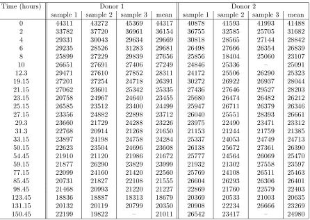
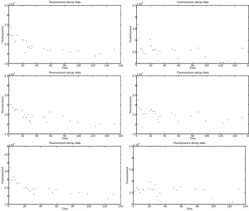
CFSE Data Set
Table 1, and plotted in Figure 1.
Time (hours) Donor 1 Donor 2
sample 1 sample 2 sample 3 mean sample 1 sample 2 sample 3 mean
0 44311 43272 45369 44317 40878 41593 41993 41488
2 33782 37720 36961 36154 36755 32585 25705 31682
4 29331 30043 29634 29669 30818 28565 27144 28842
6 29235 28526 31283 29681 26498 27666 26354 26839
8 25899 27229 29839 27656 25856 18404 25060 23107
10 26651 27691 27406 27249 24846 25336 – 25091
12.3 29471 27610 27852 28311 24172 25506 26290 25323 19.15 27201 27254 24718 26391 30272 26922 26937 28044 21.15 27062 23601 25342 25335 27436 27646 29527 28203 23.15 20758 24967 24640 23455 25680 26474 26482 26212 25.15 26585 23512 23400 24499 25947 26711 26379 26346 27.15 23356 24882 22898 23712 26040 25551 28393 26661 29.3 23660 21729 24288 23226 23975 22490 23471 23312 31.3 22768 20914 21268 21650 21153 21244 21759 21385 33.15 23897 24198 24758 24284 25337 24053 24749 24713 50.15 22623 23504 24696 23608 26138 25672 27361 26390 54.45 21910 21120 21986 21672 25777 24564 26069 25470 59.15 21877 26290 23829 23999 21932 21302 27558 23597 77.15 22099 24160 21420 22560 25769 24108 26511 25463 85.45 20731 21827 22108 21555 26604 26293 26306 26401 98.45 21468 20993 21220 21227 22869 21760 22579 22403 123.45 18836 18887 18313 18679 20369 20533 21003 20635 131.15 20132 20119 20799 20350 20908 22234 26666 23269
150.45 22199 19822 – 21011 26542 23417 – 24980
0 20 40 60 80 100 120 140 160 1.5 2 2.5 3 3.5 4 4.5x 10
4
Time
Fluorescence
Fluorescence decay data
0 20 40 60 80 100 120 140 160
2 2.5 3 3.5 4 4.5x 10
4
Time
Fluorescence
Fluorescence decay data
0 20 40 60 80 100 120 140 160
1.5 2 2.5 3 3.5 4 4.5x 10
4
Time
Fluorescence
Fluorescence decay data
0 20 40 60 80 100 120 140 160
1.5 2 2.5 3 3.5 4 4.5x 10
4
Time
Fluorescence
Fluorescence decay data
0 20 40 60 80 100 120 140
1.5 2 2.5 3 3.5 4 4.5
5x 10 4
Time
Fluorescence
Fluorescence decay data
0 20 40 60 80 100 120 140
2 2.5 3 3.5 4 4.5x 10
4
Time
Fluorescence
Fluorescence decay data
3
Mechanistic Models of Growth and Decay
In the following sections, we examine and explain the characteristic features of four main types of differential equation representations that are frequently used to model growth and decay in dynamical systems of equations. The first is an exponential (also called Malthusian) growth and decay model, for which a population is assumed to grow at a rate proportional to the size of the population at any given time [3, 4, 12, 14, 20]. The second is Michaelis-Menten kinetics, which emulates enzyme mediated kinetics. Finally, we use the Gompertz and logistic (also called Verhulst-Pearl) rate laws, which both involve time dependent growth/decay rates.
3.1
Exponential Growth and Decay
Many of the mechanistic terms used in this paper were formulated using an exponential growth or decay rate. In these systems, the change in population size is directly proportional to the population size at any given time:
dP
dt =kP. (1)
Using separation of variables, the solution to (1) is found to be
P(t) =P0ekt, (2)
where P0 is the concentration of the population at t = 0 (initial population concentration). Although the
exponential model is simple to implement, it poses a problem in the sense that it creates an unbounded solution because of the constant intrinsic or per capita growth/decay rates
dP dt
P =k. (3)
Such rates are unlikely to occur in nature or specifically in a population of cells. To more accurately model the conversion of one molecule to another, Michaelis-Menten kinetic rates can be used. As we shall explain below, one can also turn totime varyingrates where the growth/decay slows as the size of the population grows/decays.
3.2
Michaelis-Menten Kinetics
In a Michaelis-Menten reaction, the rate of product concentration [P] will initially be proportional to the initial concentration of a substrate [S]. However, as the concentration of the substrate increases, the rate will lose this proportionality and approach a maximum velocity,Vmax. The rate equation for this product formation is given
by
d[P(t)]
dt =
Vmax[S] km+ [S]
. (4)
3.2.1 Michaelis-Menten Derivation
dS
dt =−kfES+krC dE
dt =−kfES+krC+kcatC dC
dt =kfEF −krES−kcatC dP
dt =kcatC. (5)
Although not the original derivation of Michaelis Menten kinetics, George Briggs and John Haldane [3, 8, 20] came up with an alternate derivation in 1925 in which they assumed that the rate of change of C was negligible in
comparison to the rate of change of S. Accordingly, they assumed that dC
dt ≈0. Thus,kfES−krC−kcatC≈0,
which implies that
C= kf
kr+kcat
ES, (6)
meaning that dP
dt =kcat
kf kr+kcat
ES
. If we definekm=
kr+kcat kf , then dP dt = kcat km ES. (7)
Thus, we now have an equation for the rate of growth for the product in terms of the concentrations of the enzyme and substrate. However it would be better if we could find the rate in terms of only the concentration of the substrate. To solve for E, we may substitutekmand (6) into the enzyme conservation law
E0=E+C=E+
kf kr+kcat
ES=E
1 + S
km
which yields
E= E0 1 + kSm.
Now that we have a formula for E, we may substitute it into (7), and find that if we defineVmax =kcatE0, we
obtain dP dt = Skcat km E0
1 + S
km
=kcatSE0
km+S
= VmaxS
km+S .
Under the same assumptions, we find dS
dt to be the negative of dP
dt using (6):
dS
dt =−kfES+krC=−Ckr−Ckcat+Ckr=−kcatC
=−kcat
kfES kr+kcat
=−kcatES
km
=−VmaxS
where km is the amount of substrate required for the rate to reach half of Vmax and S is the concentration of
substrate [2, 3, 20]. Note that if km is significantly greater than S, then this equation may approximate the
exponential function, wherek is substituted for Vmax
km
.
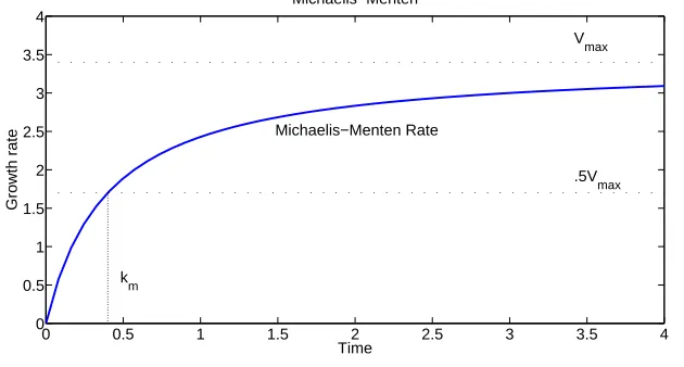
A plot of a Michaelis-Menten reaction is given in Figure 2. Although this may not be applicable for all of the reactions since some are not enzyme-mediated, it may work as a function with a bounded rate and requires only two parameter estimates. Alternatives such as the Gompertz and logistic (Verhulst-Pearl) laws also require only two parameters but, as we shall see next, offer the possible advantages of time-dependent growth/decay rates.
0 0.5 1 1.5 2 2.5 3 3.5 4
0 0.5 1 1.5 2 2.5 3 3.5 4
Michaelis−Menten
Time
Growth rate
V max
.5Vmax
k m
Michaelis−Menten Rate
Figure 2: The rate of a Michaelis-Menten reaction with km= 0.4 andVmax= 3.4.
3.3
Logistic (Verhulst-Pearl) Growth/Decay
Another model that frequently characterizes population growth/decay is the logistic growth formulation. Under this growth assumption, the change in population size at a given time is given by:
dP(t)
dt =αP(t)(1− P(t)
K ), (8)
whereα >0 is the growth/decay rate andK is thecarrying capacityfor the population.
One can readily derive the following properties for logistic models:
• The growth/decay rate (intrinsic or per capita rate) is given by
˙
P P =α
1−P(t)
K
.
• At small values of initial population (i.e., asP0 →0+), we have
˙
P P =α
1−P(t)
K
→α; so initial rates remain bounded!
3.4
Gompertz Growth/Decay
The Gompertz law is again a mathematical model in which the rate of growth/decay is greatest at the start and slowest at the end. The dynamics are given by
dP(t)
dt =αln( K
P(t))P(t) =α[ln(K)−ln(P(t))]P(t), (9) where K is the carrying capacity (upper/lower asymptote) of the population P(t) and α > 0 is the intrinsic growth/decay rate. Either of these forms in (9) can be used in our mathematical modeling. The Gompertz law is often used to model the growth of tumors as well as for population growth, but it has described label loss rate well in previous studies [5, 21], and therefore will be a candidate model for comparison in our investigations. Characteristics for Gompertz rates can summarized by:
• The growth/decay rate (per capita) is
˙
P
P =α[
ln
K−ln
P] =αln
( K P).• The solution is given by
P(t) =Ke(ln(PK0)e
(−αt)) .
• The solution has a flex point at
K e.
• At small values of initial population (i.e., asP0 → 0+), we have
˙
P P = αln
K
P → ∞ ; so initial rates can
approach unbounded values!
4
Modeling
In order to better understand the process of label decay in a cell treated with CFSE, we carried out a series of ordinary least squares (OLS) inverse problems (see [4]). A brief summary of this OLS procedure is given below in Section 4.1, and then is implemented for each of the given models in the subsequent sections. Each of these models is accompanied by a plot of total fluorescence versus time calculated by the model as compared to the data, as well as a plot of the individual mass compartments (versus time) of the components that make up this total. Although we have run the inverse problem on each model with every data set, we have only included here the plots from one data set for each model.
4.1
Overview of Inverse Problems and Model Comparison
Using the given data sets shown in Figure 1, one may carry out inverse problem procedures. This consists of estimating the vector, ~θ, which is composed of each of the unknown parameters involved in the corresponding mathematical model. The following procedure was implemented for all of the given models in order to find the most accurate fit to the data.
The inverse problem begins with a mathematical model based on the biological system. Solving this system of differential equations will produce a solution trajectory of the form~x(t, ~θ) = [x1(t, ~θ), x2(t, ~θ), . . . , xn(t, ~θ)] over
data shown in Figure 1 only gives the overall fluorescence of a population of cells, and not the value for each individual component. For this reason, we made the assumption that the overall fluorescence is composed of the individual components of the system added together. Therefore, we can designate overall fluorescence,f(t, ~θ), as:
f(t, ~θ) = (1 1 · · · 1)~x(t, ~θ). (10)
Every mathematical model requires an accompanying statistical model in order to be accurately compared to data. The statistical model is used as a way to cope with any error present in the scientific procedure, resulting from experimental, measurement, or even mathematical model error. If we assume a constant variance (CV) error, the statistical model is as follows:
~
Yj=f(tj, ~θ0) +E~j, j= 1,2,· · ·, n, (11)
wheref(t, ~θ0) corresponds to the actual solution to our mathematical model (10), andEjare independent random
variables representing the error terms. Several assumptions must hold true for our statistical model to be effective. Primarily, the true parameter, ~θ0, should actually exist. In addition, the expectation of the error terms,E[Ej],
must be zero. These two assumptions together indicate that the mathematical model accurately describes the procedure, but that the sources of error cause the observed data points to deviate from this model. The third assumption is in regards to the type of variance contained in the model. For our problem, this was given in (11) with a constant variance assumption, meaning that all throughout our model, V ar(Ej) =σ2. The error terms,
Ej also must be identically distributed, meaning that each error term is sampled from an identical probability
distribution, and thus can be denoted as identically and independently distributed, or i.i.d.[4]. Verification of this assumption is later checked in Section 5.1, which contains residual plots.
We may solve our system of equations for any value of ~θ, but our goal is to find good approximations for
~
θ0 using the data Yj. Based on the type of situation one is dealing with, there are several ways to estimateθ~0,
Given the random variable Yd
j of observations, the ordinary least squares technique can be used as an
esti-mator forθ~0 by minimizing
J(~θ) =
n
X
j=1
|Yd
j −f(tj, ~θ)|2 (12)
wheref(tj, ~θ) is the model solution at timetj with parameterθ~= k1, k2,· · · , kn. Thus, we have an estimator, ~θOLS, which we are using in hopes of finding an accurate estimate to fit to our data.
~
θOLS = arg min n
X
j=1
|Yjd−f(tj, ~θ)|2 (13)
The data set shown in Figure 1,{yj}nj=1, is then assumed to be a realization of the random variable (11). We can
implement OLS in (13) to find an estimate, ˆθOLS, which best fits our mathematical model to this data set, i.e.,
ˆ
θOLS= arg min n
X
j=1
|yj−f(tj, ~θ)|2. (14)
4.2
Biological Model 1
Due in part to the presence of two acetate esters in its structure, CFDA-SE has a high lipophilicity which allows it to passively diffuse across cell membranes [19], suggesting that both an inflow rate and an outflow rate should be accounted for. However, the data set we are examining is the result of a particular procedure where, after initial exposure to CFDA-SE, the cell culture was flushed with water, eliminating any excess label [21]. Thus, the only source of CFDA-SE inflow would be re-entering CFDA-SE, which the data suggests is insignificant. Therefore, we considered it reasonable to assume that there is no continuing flow of CFDA-SE into the cell, but rather that all CFDA-SE is present inside the cell at the start of the procedure, as depicted in Figure 3.
Once inside the cell, CFDA-SE reacts with intracellular esterases, resulting in the formation of the highly fluorescent carboxyfluorescein succinimidyl ester (CFSE). At this point, our knowledge of the reaction is limited. Nonetheless, we know a great deal about the structure of the product, CFSE. The structure of CFSE lacks the two acetate esters present in CFDA-SE [19, 21, 22]. This absence decreases the lipophilicity of CFSE and renders it less membrane permeable. As before, this knowledge necessitates both inflow and outflow rates, but the data suggests that the mass of re-entering CFSE is insignificant in comparison to the mass of CFSE leaving the cell. Therefore, only the outflow of CFSE from the cell is assumed in our model. Additionally, the succinimidyl ester present in the structure of CFDA-SE is also present in CFSE. This succinimidyl moiety of CFSE is highly reactive with amino groups and can covalently couple 5-6-carboxyfluorescein (CF) to intracellular molecules [19]. Our knowledge of this reaction and its products is currently limited, but we are aware that two types of coupling can occur, yielding two types of products. One type of coupling occurs when CF is bound to a type of intracellular molecule, which we arbitrarily call R1-NH2 that results in the conjugate CF-R1 which is unstable and quickly
exits the cell or is degraded. The second type of coupling occurs when CF is bound to a type of long lived intracellular molecule, which we arbitrarily call R2-NH2 that results in the conjugate CF-R2 that is stable and
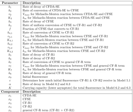
Parameter Description
k1 Rate of decay of CFDA-SE
k2 Rate of conversion of CFDA-SE to CFSE
v2 Vmax for Michaelis-Menten reaction between CFDA-SE and CFSE K2 kmfor Michaelis-Menten reaction between CFDA-SE and CFSE
k3 Rate of decay of CFSE
k4 Rate of uniform conversion of CFSE to CF-R1 and CF-R2
f Fraction of CFSE that converts to CF-R1
k4,1 Rate of conversion of CFSE to CF-R1
v4,1 Vmax for Michaelis-Menten reaction between CFSE and CF-R1 K4,1 kmfor Michaeli-Menten reaction between CFSE and CF-R1
k4,2 Rate of conversion of CFSE to CF-R2
v4,2 Vmax for Michaelis-Menten reaction between CFSE and CF-R2 K4,2 kmfor Michaelis-Menten reaction between CFSE and CF-R2
k5 Rate of decay of CF-R1
k6 Rate of decay of CF-R2
k7 Rate of conversion of CFSE to general CF-R term
v7 Vmax for Michaelis-Menten reaction between CFSE and general CF-R term K7 kmfor Michaelis-Menten reaction between CFSE and general CF-R term
k8 Rate of decay of general CF-R term
x0 Initial fluorescence
c Determines how much initial fluorescence CF-R1 & CF-R2 receive in Model 5.1
α Rate of decay in Model 6.2 and 6.3
K Carrying capacity (lower asymptote) for total fluorescence in Model 6.2 and 6.3 Component Description
x1 CFDA-SE
x2 CFSE
x3 CF-R1
x4 CF-R2
x5 general CF-R term (CF-R1 + CF-R2)
Figure 3: A schematic ofBiological Model 1, representing the serial dilution process of the intracellular dye within a cell.
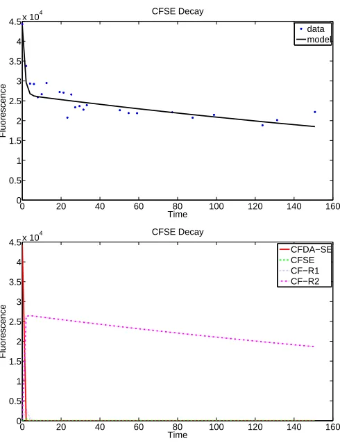
4.2.1 Model 1.1: Exponential Decay
Based on the law of mass action, the following system of equations was created to model the conversion and decay of CFDA-SE in a cell:
d~x dt =
dx1
dt =−k1x1−k2x1 dx2
dt =k2x1−k3x2−k4x4 dx3
dt =k4f x2−k5x3 dx4
dt =k4(1−f)x2−k6x4.
(15)
0 20 40 60 80 100 120 140 160 0
0.5 1 1.5 2 2.5 3 3.5 4
4.5x 10
4 CFSE Decay
Time
Fluorescence
data model
0 20 40 60 80 100 120 140 160
0 0.5 1 1.5 2 2.5 3 3.5 4
4.5x 10
4 CFSE Decay
Time
Fluorescence
CFDA−SE CFSE CF−R1 CF−R2
4.3
Biological Model 2
In the first mathematical model, Model 1.1, the rates at which CF-R1 and CF-R2 are formed from CFSE were assumed to be the same. However, based on our general knowledge of chemical reactions and energy diagrams, we questioned the appropriateness of this assumption. Typically, the rate determining step of a reaction is the step in which the most unstable state is being formed. Applying this notion to the conversion of CFSE, the reaction forming the unstable conjugate would occur much more slowly than the reaction forming the stable conjugate. Therefore, we concluded that the conversion of CFSE to CF-R1 and CF-R2 should be characterized by two different rates instead of one rate in two different proportions.
Figure 5: A schematic of Biological Model 2, with independent reaction rates from CFSE to CF-R1 and CF-R2.
4.3.1 Model 2.1: Exponential Decay
To follow this new biological model, the f parameter was removed, and the reactions of CFSE to CF-R1 and CF-R2 were treated as two completely independent reactions. This change resulted in the system of equations
d~x dt =
dx1
dt =−k1x1−k2x1 dx2
dt =k2x1−k3x2−k4,1x2−k4,2x2 dx3
dt =k4,1x2−k5x3 dx4
dt =k4,2x2−k6x4,
(16)
wherek4,1 andk4,2represent the rates of conversion to CF-R1 and CF-R2, respectively, as given in Table 2. The
plots for Model 2.1 versus the data set are presented in Figure 6.
4.3.2 Model 2.2: Michaelis-Menten Kinetics for the First Conversion
0 20 40 60 80 100 120 140 160 0 0.5 1 1.5 2 2.5 3 3.5 4
4.5x 10
4 CFSE Decay
Time
Fluorescence
data model
0 20 40 60 80 100 120 140 160
0 0.5 1 1.5 2 2.5 3 3.5 4
4.5x 10
4 CFSE Decay
Time Fluorescence CFDA−SE CFSE CF−R1 CF−R2
Figure 6: Top: A plot of Model 2.1 against the first data set from Donor 1; Bottom: the individual components versus time.
to incorporate Michaelis-Menten kinetics into our model. By substituting Michaelis-Menten kinetics for the only enzyme mediated reaction in the system (CFDA-SE to CFSE), we altered Model 2.1 to produce an alternative system given in (17). For simplicity, we have shortened allVmax,i terms tovi, and allkm,i terms will be written
asKi in order to distinguish them from the exponential rate conversion terms. The resulting model plots versus
data are given in Figure 7.
d~x dt = dx1
dt =−k1x1− v2x1
K2+x1
dx2
dt = v2x1
K2+x1−k3x2−k4,1x2−k4,2x2
0 20 40 60 80 100 120 140 160 0 0.5 1 1.5 2 2.5 3 3.5 4 4.5x 10
4 CFSE Decay
Time
Fluorescence
data model
0 20 40 60 80 100 120 140 160
0 0.5 1 1.5 2 2.5 3 3.5 4 4.5x 10
4 CFSE Decay
Time Fluorescence CFDA−SE CFSE CF−R1 CF−R2
Figure 7: Top: A plot of Model 2.2 against the first data set from Donor 1, using Michaelis-Menten kinetics for the enzyme-mediated reaction; Bottom: the different components of the system.
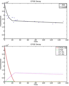
4.3.3 Model 2.3: Michaelis-Menten Kinetics for All Conversions
Although Michaelis-Menten kinetics are meant to be used to describe enzyme-mediated reactions, we thought it might be of interest to see the effects of using these kinetics to describe all three reactions in our system. The simple decay rates remain exponential, as in the previous model. This resulted in the system (18). The plots of Model 2.3 are given in Figure 8.
d~x dt = dx1
dt =−k1x1− v2x1
K2+x1
dx2
dt = v2x1
K2+x1
−k3x2−
v4,1x2
K4,1+x2
− v4,2x2
K4,2+x2
dx3
dt =
v4,1x2
K4,1+x2
−k5x3
dx4
dt =
v4,2x2
K4,2+x2
−k6x4
0 20 40 60 80 100 120 140 160 0
0.5 1 1.5 2 2.5 3 3.5 4 4.5x 10
4 CFSE Decay
Time
Fluorescence
data model
0 20 40 60 80 100 120 140 160
0 0.5 1 1.5 2 2.5 3 3.5 4 4.5x 10
4 CFSE Decay
Time
Fluorescence
CFDA−SE CFSE CF−R1 CF−R2
4.4
Biological Model 3
Upon further consideration, we generated the hypothesis that CFDA-SE is converted to CFSE through the catalyzed hydrolysis of its acetyl esters by acetylesterase. It is generally accepted that intracellular esterases are responsible for the conversion of CFDA-SE to CFSE [19, 22]. These esterases are hydrolase enzymes that cleave the acetyl esters present in CFDA-SE into their parent carboxylic acid, acetate, and an alcohol [10]. The particular esterase which specializes in removing acetyl groups is called acetylesterase [1].
Applying the mechanisms of hydrolysis to CFDA-SE produces the exact structure of CFSE that is described in the literature and Section 4.2 above. Under basic conditions, a reaction known as saponification [10] takes place (see Figure 9). First, the hydroxide, functioning as a nucleophile, attacks the electrophilic C found in the double bond of the ester, breaking the πbond and forming a tetrahedral intermediate. This intermediate then collapses to form a carboxylic acid when the alkoxide leaving group is kicked off and theπbond is re-formed. The alkoxide that was previously lost then functions as a base, quickly deprotonating the carboxylic acid and forming the final products: the parent carboxylic acid (acetate) and an alcohol.
Under acidic conditions, the reverse of Fischer esterification [10] takes place (see Figure 10). To begin with, the ester must be activated since the nucleophile present is weak and the electrophile present is poor. To do this, the oxygen of the carbonyl ester is protonated to make it more electrophilic. The molecule then encounters water, which functions as a nucleophile, attacking the electrophilic C found in the double bond of the ester, breaking the
πbond and forming a tetrahedral intermediate. Another water molecule then deprotonates the oxygen that came from the water molecule, neutralizing its charge. As with the base hydrolysis, the alkoxide needs to leave, but in this case, it is not a good enough leaving group. Therefore, it must first be protonated. Following protonation, the electrons from the adjacent oxygen help push it off, reforming the π bond and creating an alcohol. Yet another water molecule then deprotonates the oxonium ion forming the final products: the parent carboxylic acid (acetate), a regenerated acid catalyst (hydronium), and an alcohol (from the previous step). Such correlation leads us to conclude that the catalyzed hydrolysis of its acetyl esters by acetylesterase (via either mechanism above) is a reasonable explanation for the reactants and products observed in the biological process.
Figure 9: The above shows the mechanism by which the acetyl esters present in CFDA-SE are cleaved to form CFSE under basic conditions. This base hydrolysis of esters is known as saponification [10].
4.4.1 Model 3.1: Exponential decay
Based on the assumption that CFDA-SE is immediately converted to CFSE, our original exponential system was altered to only depend on five rate parameters instead of seven, yielding the system of equations (19). The variables are defined in Table 2, and depicted in the schematic for Model 3 (Figure 11). Plots of the corresponding fits-to-data are given in Figure 12.
d~x dt = dx2
dt =−k3x2−k4,1x2−k4,2x2 dx3
dt =k4,1x2−k5x3 dx4
dt =k4,2x2−k6x4.
(19)
0 20 40 60 80 100 120 140 160
0 0.5 1 1.5 2 2.5 3 3.5 4 4.5x 10
4 CFSE Decay
Time
Fluorescence
data model
0 20 40 60 80 100 120 140 160
0 0.5 1 1.5 2 2.5 3 3.5 4
4.5x 10
4 CFSE Decay
Time
Fluorescence
CFSE CF−R1 CF−R2
4.4.2 Model 3.2: Michaelis-Menten Kinetics
We again consider Biological Model 3 but with Michaelis-Menten kinetics. After applying Michaelis-Menten kinetics to all of the conversion rates and leaving the rates of decay as exponential rates, the system of differential equations (20) was created. The resulting plots versus the data along with component compartments are given in Figure 13.
d~x dt = dx2
dt =−k3x2−
v4,1x2
K4,1+x2
− v4,2x2
K4,2+x2
dx3
dt =
v4,1x2
K4,1+x2
−k5x3
dx4
dt =
v4,2x2
K4,2+x2
−k6x4.
(20)
0 20 40 60 80 100 120 140 160
0 0.5 1 1.5 2 2.5 3 3.5 4 4.5x 10
4 CFSE Decay
Time Fluorescence data model 1 1.5 2 2.5 3 3.5 4
4.5x 10
4 CFSE Decay
Fluorescence
Figure 14: A schematic of Biological Model 4, in which the two CF-R1 and CF-R2 components combined as a single component.
4.5
Biological Model 4
Encouraged by our success in simplifying our model from four to three components, we decided to test this simplicity even further with several two-component systems. The first such system combines both of the CF-R1 and CF-R2 terms together as one single component. A schematic, depicted asBiological Model 4, for this model is shown in Figure 14.
4.5.1 Model 4.1: Exponential Decay
In the first mathematical model for Biological Model 4, we assume an exponential conversion rate between each term. This is given by the differential equation (21). The results of the inverse problem calculations for Model 4.1 is plotted against the third data set from Donor 1, and is given in Figure 15.
d~x dt =
dx2
dt =−k3x2−k7x2 dx5
dt =k7x2−k8x5.
(21)
4.5.2 Model 4.2: Michaelis-Menten Kinetics
In this mathematical model, we assume a Michaelis-Menten conversion rate between CFSE and the general CF-R term, composed of both CF-R1 and CF-R2. Although there is no real biological basis for using a Michaelis-Menten reaction here since there is no enzyme involved in this step, it still provides a nice bounded solution model. The differential equation system created by using Michaelis-Menten kinetics for the conversion rates and exponential decay for the decay rates is given in (22). This model was fit to the third data set from Donor 1, with results given in Figure 16.
d~x dt =
dx2
dt =−k3x2− v7x2
K7+x2
dx5
dt = v7x2
K7+x2 −k8x5.
0 20 40 60 80 100 120 140 160 1
1.5 2 2.5 3 3.5 4 4.5x 10
4 CFSE Decay
Time
Fluorescence
model data
0
50
100
150
0
2
4
x 10
4CFSE Decay
Time
Fluorescence
CFSE
CFRs
0 20 40 60 80 100 120 140 0
0.5 1 1.5 2 2.5 3 3.5 4
4.5x 10
4 CFSE Decay
Time
Fluorescence
data model
0
50
100
150
0
1
2
3
4
x 10
4CFSE Decay
Time
Fluorescence
CFSE
CFRs
Figure 17: Schematic ofBiological Model 5, which only accounts for the fluorescence given by CF-R1 and CF-R2.
4.6
Biological Model 5
We next considered a second two-component system, where we solely assume that fluorescence is composed of the CF-R1 and CF-R2 terms, which are constantly decaying. ThisBiological Model 5 is depicted in Figure 17.
4.6.1 Model 5.1
There is only one mathematical equation for this model, and the differential equation can actually be solved analytically very easily. Accordingly, the equation for the fluorescence is given by
x(t) =cx0e−k5t+ (1−c)x0e−k6t (23)
where the c term, 0≤c≤1, allows both components to receive some of the initial fluorescence, denoted byx0.
0 20 40 60 80 100 120 140 0
0.5 1 1.5 2 2.5 3 3.5 4
4.5x 10
4 CFSE Decay
Time
Fluorescence
model data
0 20 40 60 80 100 120 140
0 0.5 1 1.5 2 2.5 3 3.5 4
4.5x 10
4 CFSE Decay
Time
Fluorescence
CF−R! CF−R2
4.7
Biological Model 6
In order to further test simplification in our models, we decided to carry out the inverse problem for the data sets using models with only one differential equation instead of an entire system. In our previous models, we were able to plot each of the components of CFSE and make predictions about how the mass of each component changes as the dye is converted from one form to another. The models in this section do not allow us to calculate the mass of each component, but they do tell us the rate of change in the total fluorescence in the cell.
4.7.1 Model 6.1: Exponential Decay
Using the exponential decay model, we created the differential equation with only one rate parameter given by
dx
dt =rx. (24)
Initial attempts at fitting the data with a fixed initial condition of the first data point resulted in exponential curves that cut through the middle of the data. We found that adding an additional parameter for estimating the initial condition allowed the exponential curve to fit the data much more smoothly, resulting in a smaller cost function but still not a convincing fit-to-data. This fit can be seen in Figure 19 against two different data sets.
0
50
100
150
0
2
4
6
x 10
4
Time
Fluorescence
CFSE decay
data
model
2
3
4
5
x 10
4
Fluorescence
CFSE decay
dx
dt =αx(1− x
K), (25)
whereαis the decay rate andK is the carrying capacity of the population, as given in Table 2. A plot for Model 6.2 versus the data is given in Figure 20.
0 20 40 60 80 100 120 140 160
0 0.5 1 1.5 2 2.5 3 3.5 4 4.5x 10
4 CFSE Decay
Time
Fluorescence
data model
0 20 40 60 80 100 120 140 160
0 0.5 1 1.5 2 2.5 3 3.5 4 4.5x 10
4 CFSE Decay
Time
Fluorescence
data model
Figure 20: Model 6.2 fit to the second data set from Donor 1 (top) and the third data set from Donor 2 (bottom), using logistic decay and one component.
4.7.3 Model 6.3: Gompertz Decay
We next used the Gompertz model to describe fluorescence decay, which has the same two parameters as Model 6.2. A plot of Model 6.3 against the data is given in Figure 21 with the equation given by
dx
dt =αxlog K
0
50
100
150
0
2
4
6
x 10
4
Time
Fluorescence
CFSE decay
data
model
0
50
100
150
2
3
4
5
x 10
4
Time
Fluorescence
CFSE decay
data
model
5
Statistical Analysis for Model Comparison
In this effort, a total of twelve different models have been introduced, raising several questions: How do we determine which of these is the most efficient fit to the data? Is a model with fewer parameters and a larger cost function better or worse than a model with more parameters and a lower cost function? How certain can one be that the model they find to be the best is actually the best model? The Akaike Information Criterion (AIC) gives an approximately unbiased form of the Kullback-Leibler Distance, or a measure of the distance between a model and the corresponding data. It is valid only for models with independent and normally distributed errors [9]. The form of the AIC measure is given by
AIC=nln J(~θOLS)
n
!
+ 2p, (27)
wherepis the number of parameters used in a model andnis the number of sample points in the data set. The AIC, however, is assumed to only be valid asymptotically and may fail when there is a small ratio of sample points to parameters (usually estimated aroundn/p <40). Since the CFSE decay data only has 24 time points, the AIC is most likely biased in this situation. For this reason, Hurvich and Tsai [9] created a small sample adjustment, labeledAICC given by
AICC=nln
J(~θOLS) n
!
+ 2p+2p(p+ 1)
n−p−1. (28)
Once AICC values have been computed for each model, it is important to find the likelihood that each model
is actually the best fit for the data. It is a general rule that the smallestAICC value corresponds to the model
which most efficiently matches the given data set. It is also important to calculate the likelihood that each of the other models is actually the best. The model with lowestAICC value is denoted asAICC,min. This relative
likelihood that modeliis a better fit than the AICC,min model can be calculated using
RLi=e 1
2(AICC,min−AICC,i). (29)
A more intuitive method for showing how likely each model is to be the most accurate is Akaike weights, in which each model’s relative likelihood is divided by the sum of all the likelihoods, or
wi= RLi
4
P
m=1
RLm
. (30)
5.1
Results
The AIC is a useful tool for selecting the best model approximation from a set of different models, but it is important to note that the AIC should only be used for comparison. One single AIC value has no meaning in itself. If the AIC is used for a set of poorly made models, then it will still choose a poor model as the best fit, so it is crucial for the modeler to ensure that the given models are well founded [9].
The calculated AICc and wi values for each of the six data sets are given in Tables 3 - 8, and the residual
0 20 40 60 80 100 120 140 −3000 −2000 −1000 0 1000 2000 3000 Residual Plot Time
data − model
0 20 40 60 80 100 120 140
−4000 −3000 −2000 −1000 0 1000 2000 3000 4000 Residual Plot Time
data − model
0 20 40 60 80 100 120 140
−3000 −2000 −1000 0 1000 2000 3000 Residual Plot Time
data − model
0 20 40 60 80 100 120 140
−6000 −4000 −2000 0 2000 4000 6000 Residual Plot Time
data − model
0 20 40 60 80 100 120 140
−3000 −2000 −1000 0 1000 2000 3000 Residual Plot Time
data − model
0 20 40 60 80 100 120 140
−4000 −3000 −2000 −1000 0 1000 2000 3000 4000 Residual Plot Time
data − model
0 20 40 60 80 100 120 140 −4000
−3000 −2000 −1000 0 1000 2000 3000 4000
Residual Plot
Time
data − model
0 20 40 60 80 100 120 140
−4000 −3000 −2000 −1000 0 1000 2000 3000 4000
Residual Plot
Time
data − model
0 20 40 60 80 100 120 140
−5000 0 5000
Residual Plot
Time
data − model
0 20 40 60 80 100 120 140
−3 −2 −1 0 1 2 3
x 104 Residual Plot
Time
data − model
0 20 40 60 80 100 120 140
−5000 0 5000
Residual Plot
Time
data − model
0 20 40 60 80 100 120 140
−5000 0 5000
Residual Plot
Time
data − model
Model p J(ˆθOLS) AICC wi
1.1 8 9.988×10⁷ 391.39 0.000
2.1 8 4.940×10⁷ 374.50 0.000 2.2 9 4.923×10⁷ 379.67 0.000 2.3 11 9.232×10⁷ 407.91 0.000 3.1 6 3.0388×10⁷ 354.18 0.9972
3.2 8 4.925×10⁷ 374.43 0.0000 4.1 4 7.069×10⁷ 367.60 0.0012 4.2 5 7.070×10⁷ 370.84 0.0002
5.1 3 7.070×10⁷ 367.61 0.0012 6.1 3 3.728×10⁸ 404.61 0.000 6.2 3 1.217×10⁸ 377.74 0.000 6.3 3 1.095×10⁸ 375.21 0.000
Table 3: Statistical results for the first data set from Donor 1, with best in bold
Model p J(ˆθOLS) AICC wi
1.1 8 5.793×10⁷ 378.32 0.002
2.1 8 5.819×10⁷ 378.43 0.002 2.3 9 5.298×10⁷ 381.43 0.0000 2.3 11 6.0243×10⁷ 397.66 0.000
3.1 6 5.849×10⁷ 369.89 0.0126 3.2 8 5.891×10⁷ 378.72 0.0002 4.1 4 5.774×10⁷ 362.75 0.4483 4.2 5 5.849×10⁷ 366.29 0.0765
5.1 3 5.775×10⁷ 362.75 0.4479 6.1 3 3.836×10⁸ 405.29 0.000 6.2 3 9.454×10⁷ 371.68 0.0052
6.3 3 9.026×10⁷ 370.56 0.0090
Table 4: Statistical results for the second data set from Donor 1, with best in bold
Model p J(ˆθOLS) AICC wi
1.1 8 3.394×10⁷ 365.49 0.0000 2.1 8 4.048×10⁷ 369.72 0.0000 2.2 9 3.000×10⁷ 367.75 0.0000 2.3 11 5.244×10⁷ 382.71 0.0000 3.1 6 3.358×10⁷ 356.57 0.0002
Model p J(ˆθOLS) AICC wi
1.1 8 1.223×10⁸ 396.25 0.0000
2.1 8 1.108×10⁸ 393.89 0.0001 2.2 9 1.075×10⁸ 398.43 0.0000 2.3 11 3.270×10⁸ 438.26 0.0000 3.1 6 1.165×10⁸ 386.44 0.0048
3.2 8 1.096×10⁸ 393.62 0.0001 4.1 4 1.110×10⁸ 378.43 0.2638 4.2 5 1.097×10⁸ 381.37 0.0605
5.1 3 1.110×10⁸ 378.43 0.2634 6.1 3 3.671×10⁸ 404.23 0.000 6.2 3 1.251×10⁸ 378.41 0.2664 6.3 3 1.320×10⁸ 379.69 0.1403
Table 6: Statistical results for the first data set from Donor 2, with best in bold
Model p J(ˆθOLS) AICC wi
1.1 8 1.143×10⁸ 394.64 0.0002
2.1 8 1.221×10⁸ 396.21 0.0001 2.2 9 1.212×10⁸ 401.29 0.0000 2.3 11 4.5191×10⁸ 446.02 0.0000
3.1 6 1.230×10⁸ 387.74 0.0050 3.2 8 1.101×10⁸ 393.73 0.0002 4.1 4 1.167×10⁸ 379.64 0.2862 4.2 5 1.215×10⁸ 383.76 0.0365
5.1 3 1.167×10⁸ 376.43 0.2863 6.1 3 3.765×10⁸ 404.84 0.0000 6.2 3 1.331×10⁸ 379.88 0.2538
6.3 3 1.406×10⁸ 381.19 0.1317
Table 7: Statistical results for the second data set from Donor 2, with best in bold
Model p J(ˆθOLS) AICC wi
1.1 8 8.689×10⁷ 361.24 0.0000 2.1 8 8.481×10⁷ 360.70 0.0000 2.2 9 8.464×10⁷ 366.58 0.0000 2.3 11 8.346×10⁷ 381.67 0.0000 3.1 6 8.651×10⁷ 351.67 0.0025 3.2 8 8.464×10⁷ 360.66 0.0000 4.1 4 7.924×10⁷ 342.49 0.2470
4.2 5 8.461×10⁷ 347.32 0.0220 5.1 3 7.924×10⁷ 342.49 0.2470 6.1 3 2.903×10⁸ 368.03 0.0000 6.2 3 9.515×10⁷ 343.49 0.1494 6.3 3 8.849×10⁷ 341.89 0.3320
6
Concluding Remarks
After careful examination of related chemical processes and biological processes, twelve different mathematical models were formulated and analyzed for the rate of label decay in a cell treated with carboxyfluorescein diacetate succinimidyl ester (CDSA-SE). It is important to note that CFDA-SE was disregarded after Biological Models 1 and 2, based on the assumption that CFDA-SE is converted to CFSE at a quickly catalyzed rate. The esterase reaction was hypothesized to specifically involve the enzyme acetylesterase, which binds to acetic ester and water, giving alcohol and acetate as products. This knowledge led us to incorporate Michaelis-Menten kinetics to support the hypothesis that there is no inflow of CFDA-SE and determine the rate of its conversion to CFSE. Logistic decay and Gompertz decay were also used to model the decay of the total fluorescence. Although no model was the best fit for every data set, our results suggest that Models 3.1, 4.1, 5.1, and 6.3 are the models that most closely match the data. All of these models involve either multiple rates of label leaking/decay or a time dependent rate for the decay of a single label quantity. This project provides a reasonable explanation in support of the multiple decay rates observed in data involving CFSE labeling.
7
Acknowledgements
This research was supported in part by grant number NIAID R01AI071915-09 from the National Institute of Allergy and Infectious Diseases and in part by the Undergraduate Biomathematics grant number NSF DBI-1129214 from the National Science Foundation. The authors are also most grateful to Jordi Argilaguet and Cristina Peligero of the ICREA Infection Biology Lab, Univ. Pompeu Fabra, Barcelona, Spain for generously providing the experimental data used in this study.
References
[1] Acetyl Esterase [Internet]. CPC Biotech S.r.l. 2007-2011. [cited 2012 Jun 07]. Available from: http://www.cpcbiotech.it/EN/c/d/enzyme-portfolio/enzymes/acetyl-esterase-lyophilized
[2] Peter Atkins and Julio De Paula,Physical Chemistry (9th edition), Freeman, New York, 2010.
[3] H.T. Banks, Modeling and Control in the Biomedical Sciences, Lecture Notes in Biomathematics, Vol. 6, Heidelberg, Springer, 1975.
[4] H.T. Banks and H.T. Tran,Mathematical and Experimental Modeling of Physical and Biological Processes, CRC Press, Boca Raton London New York, 2009.
[5] H.T. Banks, Karyn L. Sutton, W. Clayton Thompson, Gennady Bocharov, Marie Doumic, Tim Schenkel, Jordi Argilaguet, Sandra Giest, Cristina Peligero, and Andreas Meyerhans, A new model for the estimation of cell proliferation dynamics using CFSE Data, CRSC-TR11-05, NCSU, August, 2011; J. Immunological Methods,373(2011), 143–160.
[10] F. Carey,Organic Chemistry, 8th edition, McGraw-Hill, New York, 2011.
[11] William W. Chen, Mario Niepel and Peter K. Sorger, Classic and contemporary approaches to modeling biochemical reactions,Genes & Development,24 (2010), 1861–1875.
[12] Gerda de Vries, et al., A Course in Mathematical Biology, SIAM Series on Mathematical Modeling and Computation, Vol.MM12, SIAM, Philadelphia, 2006.
[13] J. Hasenauer, D. Schittler and F. Allg¨ower, Analysis and simulation of division- and label-structured popu-lation models: A new tool to analyze proliferation assays,Bull. Math. Biol., 74(2012), 2692–2732.
[14] M. Kot,Elements of Mathematical Ecology, Cambrodge University Press, Cambridge, UK, 2001.
[15] A. B. Lyons, Divided we stand: tracking cell proliferation with carboxyfluorescein diacetate succinimidyl ester,Immunology and Cell Biology,77 (1999), 509–515.
[16] A. B. Lyons, J. Hasbold and P.D. Hodgkin, Flow cytometric analysis of cell division history using diluation of carboxyfluorescein diacetate succinimidyl ester, a stably integrated fluorescent probe, Methods in Cell Biology, 63(2001), 375–398.
[17] A. B. Lyons and K. V. Doherty, Flow cytometric analysis of cell division by dye dilution, Current Protocols in Cytometry, (2004), 9.11.1-9.11.10.
[18] A.B. Lyons and C.R. Parish, Determination of lymphocyte division by flow cytometry,J. Immunol. Methods, 171(1994), 131–137.
[19] C. Parish, Fluorescent dyes for lymphocyte migration and proliferation studies,Immunology and Cell Biology 77(1999), 499–508
[20] S. I. Rubinow,Introduction to Mathematical Biology, J. Wiley & Sons, New York, 1975.
[21] W. Clayton Thompson, Partial Differential Equation Modeling of Flow Cytometry Data from CFSE-based Proliferation Assays, Ph.D. Dissertation, Dept. Mathematics, North Carolina State University, December, 2011.