ABSTRACT
DIDWANIA, KAUSHAL. Performance Evaluation of Greenplum in VCL Cloud Computing Environment. (Under the direction of Dr. Mladen Vouk.)
Large amounts of data are becoming a way of life. Data is used to make important decisions, and the rate of data acquisition requires not only large amounts of storage, but also an ability to analyze that data, search it and otherwise mine that information. This is true in practically any type of domain health care, science analytics, security, shopping, advertising, etc. Some of the major challenges involve real-time response, storage capacity, processing, network latency (especially for data in the cloud), scalability, etc. The key element in managing this data tsunami is often a high quality high-speed data base, something that may not be readily available to an average user. In fact, an essential component of any cloud is its ability to collect a lot provenance information and store in an easily retrievable way in database(s). This thesis is concerned with integration of high-performance high-capacity databases into a cloud environment - either as part of the cloud system, or as part of end-user applications.
studied the behavior and performance of Greenplum Community edition (free) under a variety of conditions including the number to data servers, number of interconnects, cluster size, etc., and measured its performance and performance of its components (networks, disk I/O, etc.) using standard metrics and benchmarks (such as TPC-H) to identify bottlenecks and issues, as well as solutions.
c
Copyright 2012 by Kaushal Didwania
Performance Evaluation of Greenplum in VCL Cloud Computing Environment
by
Kaushal Didwania
A thesis submitted to the Graduate Faculty of North Carolina State University
in partial fulfillment of the requirements for the Degree of
Master of Science
Computer Science
Raleigh, North Carolina 2012
APPROVED BY:
Dr. Vincent W. Freeh Dr. Rada Y. Chirkova
DEDICATION
BIOGRAPHY
Kaushal Didwania was born in a Kolkata, West Bengal in India. He received his Bachelors in Computer Engineering from Vishwakarma Institute of Technology which is affiliated with Pune University in May 2005. After completion of his Bachelors he pursued his Masters in Computer Science in North Carolina State University from August 2010 to May 2012.
ACKNOWLEDGEMENTS
I thank my parents, my brother and my sister for their unwavering support and rock-steady faith in me. I would not have made it without their constant encouragement and motivation.
I am deeply grateful to my adviser Dr. Mladen Vouk for knowing where my interests lay and for orienting me in those directions. In addition to his many useful suggestions and constant guidance, I cherish the trust he placed in me, and the freedom I was allowed during the course of this work. I would like to thank Dr. Vincent Freeh for making his courses both fun and valuable and Dr. Rada Chirkova for her valuable help and guidance in helping me benchmarking the database & for graciously agreeing to be in the thesis committee. Special thanks are due to Aaron Peeler as well, for helping me to obtain cluster reservations in VCL.
TABLE OF CONTENTS
List of Tables . . . vii
List of Figures . . . viii
Chapter 1 Introduction . . . 1
1.1 Motivation . . . 1
1.2 Data Warehousing . . . 2
1.3 EMC’s Greenplum . . . 3
1.4 Comparison of Greenplum with other Vendors . . . 4
Chapter 2 Background . . . 6
2.1 Study of Greenplum . . . 6
2.1.1 Greenplum Architecture . . . 7
2.1.2 Network Topology . . . 8
2.1.3 Data Distribution and Parallel Scanning . . . 9
2.1.4 Storage and File System . . . 11
2.2 Benchmarking Databases . . . 11
Chapter 3 Experimental Setup . . . 12
3.1 Configuration of Nodes in VCL . . . 13
3.2 Database in a Cloud . . . 13
3.3 Installation of Greenplum . . . 16
3.3.1 Pre-Configuration required in VCL images . . . 16
3.3.2 Setting of Kernel Parameters . . . 16
3.3.3 Installation of Greenplum in Master Host . . . 17
3.3.4 Installation of Greenplum on all hosts . . . 17
3.3.5 Creating Data Storage Areas . . . 18
3.3.6 Synchronizing System Clocks . . . 19
3.3.7 Post-Configuration required in VCL images . . . 19
3.4 System Specifications of Machines Configured . . . 20
3.5 Architecture of Configured System . . . 20
3.5.1 Configuration 1 . . . 21
3.5.2 Configuration 2 . . . 21
3.5.3 Configuration 3 . . . 24
Chapter 4 Experimental Results . . . 25
4.1 Validating installation . . . 25
4.1.1 Validating OS settings . . . 25
4.2 Validating I/O Performance . . . 29
4.3 Storage Models . . . 30
4.4 Performance Analysis . . . 31
Chapter 5 Conclusion and Future Work . . . 35
5.1 Conclusion . . . 35
5.2 Future Work . . . 37
References . . . 38
Appendices . . . 40
Appendix A Loading and Testing Scripts . . . 41
A.1 /etc/init.d/vcl post reserve . . . 41
A.2 testScript.sh . . . 45
Appendix B Run Time Instances . . . 48
Appendix C Results obtained from Greenplum Images . . . 52
C.1 Loading and Execution Results . . . 52
C.2 Network Performance on Private Interface . . . 52
LIST OF TABLES
Table 4.1 Loading and Execution Times . . . 31
Table C.1 Loading and Execution Times for Configuration 1 . . . 53
Table C.2 Loading and Execution Times for Configuration 2 . . . 54
Table C.3 Loading and Execution Times for Configuration 3 . . . 56
Table C.4 Network Performance on Private Interface . . . 58
Table C.5 Network Performance Across Reservations . . . 59
Table D.1 PART Table Layout . . . 61
Table D.2 SUPPLIER Table Layout . . . 62
Table D.3 PARTSUPP Table Layout . . . 62
Table D.4 CUSTOMER Table Layout . . . 62
Table D.5 NATION Table Layout . . . 62
Table D.6 ORDERS Table Layout . . . 63
Table D.7 LINEITEM Table Layout . . . 63
Table D.8 REGION Table Layout . . . 63
LIST OF FIGURES
Figure 2.1 Architecture of Greenplum . . . 8
Figure 2.2 GNet Interconnect . . . 9
Figure 2.3 Automatic hash-based data distribution . . . 10
Figure 3.1 Architecture of VCL Nodes . . . 14
Figure 3.2 Experiment Architecture for Configuration 1 . . . 22
Figure 3.3 Experiment Architecture for Configuration 2 . . . 23
Figure 3.4 Experiment Architecture for Configuration 3 . . . 24
Figure 4.1 Network Performance for Serial Workload on VCL Public interface 27 Figure 4.2 Network Performance for Parallel Workload on VCL Public interface 28 Figure 4.3 Network Performance for Matrix Workload on VCL Public interface 29 Figure 4.4 Loading and Execution Time on different Cluster Size . . . 32
Figure 4.5 Loading and Execution Time on different Configuration . . . 33
CHAPTER
1
Introduction
1.1
Motivation
row-oriented fashion. For queries on vast amounts of data, traditional relational databases such as Oracle, MySQL, or PostgreSQL may not the best choice because most of the relational database management systems were originally designed for on-line transaction workloads and may not represent large-scale analytics workloads. Large-scale analytics workload queries include data attributes which are field oriented compared to general insert or update queries which are record oriented. Because of the difference in workloads, a different architecture, a column-oriented distributed one may be desirable.
1.2
Data Warehousing
1.3
EMC’s Greenplum
To deal with problems mentioned above that arises with large-scale data housed on single instances of a database, we turn to distributed databases. In the latter many distinct database instances cooperate over a single, perhaps redundant, DBMS to form a single logical database that is in reality physically distributed over multiple computers and possibly different sites. Greenplum[3, 4] is such a solution built to support the next generation of data warehousing and large-scale analytics processing. It is a massively parallel processing (MPP) database which is based on a shared nothing architecture. By shared nothing architecture, it means that when data is loaded into the segments, it is divided based on a distributer function and hence, each of its segment servers contains only a part of the entire data. Each segment acts as a self-contained database and is only responsible for the part of data it stored. Now, when a query is to be executed, it is executed simultaneously on all of its segments decreasing the execution time by the number of nodes on which data is kept and thus, making Greenplum a shared nothing architecture.
Some additional features provided by Greenplum are complex query optimization, parallel data loading, fault tolerance, workload management, administration and mon-itoring, etc. Quoting from Greenplum’s White Paper titled Critical Mass Innovation ”Its is conceived, designed, and engineered to allow customers to take advantage of large clusters of increasingly powerful, increasingly inexpensive commodity servers, storage, and
Ethernet switches. Greenplum customers can gain immediate benefit from deploying the
1.4
Comparison of Greenplum with other Vendors
Of course, Greenplum is not the only distributed database. Some of the popular ones are Teradata from Teradata[5], Exadata from Oracle[6], Aster Database from Aster Data[7], etc.
Unlike Teradata, Greenplum provides a software only solution. It means we can get only the software of Greenplum and install it in the machines we have and configure it accordingly to run based on available processing speed. Greenplum integrates the interconnect network from Cisco, and storage servers from EMC and the processing power from Intel, so they don’t have to spend a lot of money in the R&D to enhance their configuration. It also makes Greenplum very flexible in choosing the products they want to install. However, their initial cost is high since everything has to be brought from different companies and installed. Teradata is a highly tightly coupled system which means they design their entire interconnect, their storage servers and the processors which needs to be embedded inside. Although it makes their initial cost less compared to Greenplum but they spends a lot on their R&D continuously to enhance their technologies.
architecture and keeps the storage and the database server in one compute node. Also, Exadata does not provide a software only solution which is provided by Greenplum.
Aster database is another interesting database when compared to Greenplum since both of them provide software-only solutions, both partner with hardware vendors and manufacture an appliance with their software installed on it, both use shared-nothing architecture and both use PostgreSQL as their underlying database. The difference between them is that Greenplum has made significant modifications to the PostgreSQL code-base while Aster Data has kept most of the original code of PostgreSQL and treats database as a black-box.
CHAPTER
2
Background
2.1
Study of Greenplum
Quoting from Greenplum’s White paper ”Greenplum Database is a software solution built to support the next generation of data warehousing and large-scale analytics processing.
Supporting SQL and Map-Reduce parallel processing, the database offers industry-leading
2.1.1
Greenplum Architecture
Since the workloads of Business Analytics queries is fundamentally different from OLTP based queries, the design of the database for managing Business Intelligence(BI) workloads should be different than Relational Database Management Systems(RDBMS) which were designed for OLTP transactions. Hence, Greenplum database utilizes a shared-nothing, massively parallel processing (MPP) architecture designed to achieve highest levels of parallelism and efficiency for Complex BI and analytical processing.
architecture can be found in Greenplum’s white paper[3].
Applications
Network Interface Master and Standby master
Segment Segment
External Data Sources Layer 1
Layer 5 Layer 4 Layer 3 Layer 2
Figure 2.1: Architecture of Greenplum
2.1.2
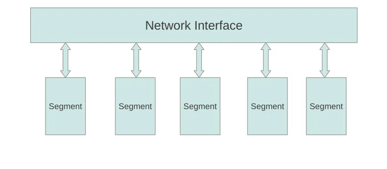
Network Topology
By default, the interconnect uses UDP (User Datagram Protocol) to send messages over the network. This, of course, is an unreliable (if fast) way of moving data and so fault-tolerance is done by Greenplum itself. The Greenplum software does the additional packet verification and checking not performed by UDP, so the reliability is equivalent to TCP (Transmission Control Protocol).
Network Interface
Segment Segment Segment Segment Segment
Figure 2.2: GNet Interconnect
2.1.3
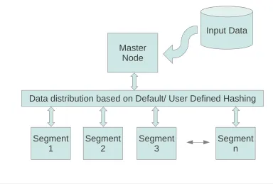
Data Distribution and Parallel Scanning
In order to maximize efficiency, data is divided and stored in the segments, based on a distribution function. While creating the tables, the function can can be user defined if distribution of data based on a certain field is required or user can use by default hashing distribution which allows all the segments to contain equal amount of data.
Once the data is loaded in the system, the process of scanning a table is dramatically faster than in other architectures because no single node needs to do all the work. All segments work in parallel and scan their portion of the table, allowing the entire table to be scanned in a fraction of the time of sequential approaches. Users aren’t forced to use aggregates and indexes to achieve performance. They can simply scan the table and get answers in unmatched time.
Input Data
Master Node
Data distribution based on Default/ User Defined Hashing
Segment
1 Segment2 Segment3 Segmentn
2.1.4
Storage and File System
Greenplum is optimized to use XFS file system. XFS is particularly proficient in handling large files and at offering smooth data transfers. However, other file systems like ext3 may be used in Greenplum depending on the architecture of the machines on which Greenplum is installed.
2.2
Benchmarking Databases
There are variety of benchmarking products like TPC[8](not to be confused with network-ing TCP protocol), Open Source Benchmarknetwork-ing, SysBench, Benchmark Factory, available in market to benchmark databases. However, distributed databases for Data Warehousing, Data Mining, etc. are benchmarked differently from traditional relational databases be-cause of their unique design and different workloads. TPC-H is one such ad-hoc, decision support benchmark which can be used to benchmark Greenplum database.
There are two executable files provided by TPC-H which are dB-Gen and q-Gen. dB-Gen is used for generating data for 8 tables namely nation, region, part, supplier, orders, lineitem, partsupp and customer and q-Gen is used for executing 22 queries provided by the benchmark for decision support. To get information on columns and datatypes of these tables and the queries which are executed refer to Appendix D.
CHAPTER
3
Experimental Setup
and then configure for their desired usage.
3.1
Configuration of Nodes in VCL
To reserve a machine a user must log in to http://vcl.ncsu.edu and then request the type of resource they want to use. For more information on reserving a machine refer to http://vcl.ncsu.edu[11]. Once the machine is reserved, it is connected through two network interfaces. A public network which is of the form 152.x.x.x through which users can access the system and perform their task. In a Linux environment, this is typically the eth1 interface. In most of the VCL-gp resources interconnects are 1Gbps cable. On the VCL HPC side there are resources that are 10Gbps Ethernet capable or Infiniband enabled. The other network is private. It is primarily used to manage resources and load images out of band. Typically it is the eth0 interface in Linux, the subnet is in the 10.x.x.x space and it is atleast 1Gbps cable. A high level view is shown if Fig 3.1. For details VCL refer to [9, 10, 12].
3.2
Database in a Cloud
One of the major challenges faced while integrating Greenplum into a Cloud environment is deciding how the end user can reserve and use Greenplum because it highly depends on the kind of Cloud environment available in terms of what resources it can leverage. Some of the methods of integrating it are:
Node eth0
eth1
Management Node Private N/w
Public N/w 152.x.x.x 10.x.x.x
function can be written to allow the users to create a different database per user and for security. Using this architecture there will be no wait time for the user because Greenplum will already be configured and available but the resources may go underutilized. It have a high cost and energy consumption.
• A loosely coupled system in which the user can take the Master Segment and the Child Segments separately and run a script to configure Greenplum. This configuration definitely has an advantage of only using the machines when it is required but it can highly effect the performance which is not desirable. Since the reservations will be taken separately, they can be allocated from anywhere in the Cloud. If the machines are allocated from different data centers, it will add a considerable amount of network delay.
• Third way of integrating Greenplum was having a flavor of both the above described methods. Having a fixed IP for the master and when the end user needs reservation. He can log into the master and initiate the number of Greenplum Segments required by him. VCL provides XMLRPC API’s which the Master Segment can leverage and take the number of reservations and Greenplum in them.
3.3
Installation of Greenplum
Following are the steps taken to install Greenplum in VCL. The steps might be different if installing in different machine or different architecture. For detailed explanation and installation on different machine refer to Greenplum installation Guide[13].
3.3.1
Pre-Configuration required in VCL images
The following steps are to be performed before installing on the images of master, standby master and segment server of Greenplum:
• A user named ’gpadmin’ with password as ’greenplum’ was created.
• An rsa key is generated in for the user ’gpadmin’.
3.3.2
Setting of Kernel Parameters
The following Linux kernel properties needs to be set in /etc/sysctl.conf file in CentOS 5.x:
kernel.sem= 250 512000 100 2048 kernel.shmmax= 500000000 kernel.shmmni= 4096 kernel.shmall= 4000000000 kernel.sem= 250 512000 100 2048 kernel.sysrq= 1
kernel.msgmni= 2048 net.ipv4.tcp syncookies= 1 net.ipv4.ip forward= 0
net.ipv4.conf.default.accept source route= 0 net.ipv4.tcp tw recycle= 1
net.ipv4.tcp max syn backlog= 4096 net.ipv4.conf.all.arp filter= 1
net.ipv4.conf.default.arp filter= 1
net.ipv4.ip local port range= 1025 65535 net.core.netdev max backlog= 10000 vm.overcommit memory= 2
3.3.3
Installation of Greenplum in Master Host
Greenplum can be downloaded from the Greenplum website and the installer can be launched using the following command:
# /bin/bash greenplum-db-4.1.x.x-PLATFORM.bin
Greenplum will be installed in /usr/local/greenplum-db-4.1.x.x/. It will create folders in the directory containing the required documents, demo, python scripts, header files, sample configuration files, the shared files for Greenplum e.t.c.
3.3.4
Installation of Greenplum on all hosts
• Log in to the master host as root:-• Source the path file from your master hosts Greenplum Database installation directory:
# source /usr/local/greenplum-db/greenplum path.sh
• Create a file called hostfile exkeys that has the machine configured host names and host addresses (interface names) for each host in your Greenplum system (master, standby master and segments). This file is need by the Greenplum Master
to configure itself with the Greenplum Segments.
• Run the gpseginstall utility using hostfile exkeys which is created.
# gpseginstall -f hostfile exkeys -u gpadmin -p P@$$word
3.3.5
Creating Data Storage Areas
Every host in Greenplum will need a storage space to load and store data. In the master a location was created and data was stored in that location. In the master as root a directory is created at /data/master/ and then gpadmin is made the owner of the directory.
For all the segment hosts the following commands are executed to create and make gpadmin as the owner. Additional steps have to be taken to create directory for the standby master or mirror segment servers. hostfile gpssh segonly is created containing the domain names of only the segment servers.
# gpssh -f hostfile gpssh segonly -e ’mkdir /data/primary’
3.3.6
Synchronizing System Clocks
Greenplum recommends using NTP (Network Time Protocol) to synchronize the system clocks on all hosts that comprise your Greenplum Database system. NTP on the segment hosts should be configured to use the master host as the primary time source, and the standby master as the secondary time source. On the master and standby master hosts, configure NTP to point to your preferred time server. Since the machines on which Greenplum images are loaded comes from same management node, this step can be avoided as the time of all the machines are synchronized.
3.3.7
Post-Configuration required in VCL images
The following steps are to be performed after greenplum is installed in the master, standby master and the segment images. The script is located at /etc/init.d/vcl post reserve. The script can also be referred from Appendix A.
• The ssh configuration files for public and private network are modified to allow root login and password less ssh.
• The same key which was saved in all the images is copied from user ’gpadmin’ to root.
• Restart the ssh to start the modified ssh files.
• Allow firewall to accept connections from segment images.
• IP addresses and their hostnames are added in /etc/hosts file to allow machines to accepts to connections.
• Hostfiles to configure greenplum are created in /usr/local/greenplum-db/hostfiles/ using information of ip addresses and domain names.
• Owner of all the hostfiles are changed to ’gpadmin’
• gpinitsystem command is issued as ’gpadmin’ to configure the new master and seg-ments. su gpadmin -c ’gpinitsystem -c /usr/local/greenplum-db/gpinitsystem config -h /usr/local/greenplum-db/hostfile gpinitsystem’ If all the steps are performed
correctly, the greenplum image is ready for the user to work.
3.4
System Specifications of Machines Configured
Greenplum was installed and evaluated in the following configuration: - 2 Intel(R) Xeon(TM) CPU 3.00GHz
- 4GB of RAM - 2MB cache size - ext3 file system
- 18GB Hard-disk space
3.5
Architecture of Configured System
were created in VCL. All the images are created to run Greenplum-db with different configurations.
The images work as a cluster where Greenplum Master(CentOS), Greenplum Master Node v2 and Greenplum Master Node v3 act as parent images and Greenplum Seg-ment(CentOS) and Greenplum Segment with Mirror act as child images. Greenplum was installed with three different configurations depending on the the network interfaces they use or if the data needs to be mirrored in the nodes. The user can load the data through the master compute node or using the gpload command which allows the Greenplum Segments to access data directly from another server.
3.5.1
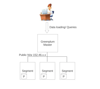
Configuration 1
The first configuration was made with images using Greenplum Master (CentOS) and Greenplum Segment (CentOS). It is configured with only one public network interface and data mirroring is not configured to protect against failures. Figure 3.2 gives a logical view of the configuration.
3.5.2
Configuration 2
Greenplum Master
Segment Segment Segment
Public N/w 152.46.x.x
Data loading/ Queries
P P P
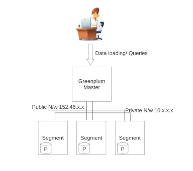
Greenplum Master
Segment Segment Segment
Public N/w 152.46.x.x
Data loading/ Queries
P P P
Private N/w 10.x.x.x
3.5.3
Configuration 3
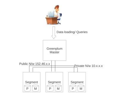
The third configuration was made with images using Greenplum Master Node v3 and Greenplum Segment with Mirror. It is configured with two network interfaces, the 152.46.x.x public interface and 10.x.x.x private interface. In this configuration data was also mirrored in the segments to provide fault tolerance. Figure 3.4 gives a logical view of the configuration. Data mirroring is done on different network interfaces if available allowing protection and access to data in case of link failures as well.
Greenplum Master
Segment Segment Segment
Public N/w 152.46.x.x
Data loading/ Queries
P P P
Private N/w 10.x.x.x
M M M
CHAPTER
4
Experimental Results
4.1
Validating installation
Greenplum provides gpcheck and gpcheckperf functions to validate the configuration and performance of Greenplum database. These utilities validates the OS setting and Hardware performance respectively.
4.1.1
Validating OS settings
A file hostfile gpcheck was created containing the hostnames of all the machines in which greenplum is installed which consists of master, standby master and all segment servers(one per line) and then gpcheck utility is executed using the following command:
After installing Greenplum in VCL and executing the command, the following was the result obtained:
gpcheck:bn18-94:root-[INFO]:-dedupe hostnames
gpcheck:bn18-94:root-[INFO]:-Detected platform: Generic Linux Cluster gpcheck:bn18-94:root-[INFO]:-generate data on servers
gpcheck:bn18-94:root-[INFO]:-copy data files from servers gpcheck:bn18-94:root-[INFO]:-delete remote tmp files
gpcheck:bn18-94:root-[INFO]:-Using gpcheck config file:$GPHOME/etc/gpcheck.cnf gpcheck:bn18-94:root-[ERROR]:-GPCHECK ERROR host(bn17-239.dcs.mcnc.org): on device (sda) IO scheduler ’cfq’ does not match expected value ’deadline’
gpcheck:bn18-94:root-[INFO]:-gpcheck completing...
The error obtained was because of the file system which was being used. Greenplum’s preferred file system is XFS but the machines in which it was installed in VCL contains ext3. Since the scheduler of ext3 and XFS, we receive an error but Greenplum is still functional.
4.1.2
Validating Hardware Performance
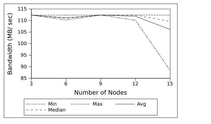
3 6 9 12 15
Number of Nodes
85 90 95 100 105 110 115
Bandwidth (MB/ sec)
Min Max Avg
Median
Figure 4.1: Network Performance for Serial Workload on VCL Public interface
master will transfer data to all the segments at the same time and matrix workload where all the segments transfer data to each other in a parallel fashion. This utility uses netperf tool to evaluate the network performance and reports the minimum, maximum, average and median network transfer rates in MB/ sec. Reading were taken with 3 times on different reservations taken at different times, to view the entire reading refer to Table C.5 in Appendix C.
Figure 4.1 displays the network bandwidth of the system for serial workload when a cluster reservation of Greenplum with 3, 6, 9, 12 and 15 segments are reserved. As the figure displays, the bandwidth to each of the system is close to 100 MB/ sec regardless of the number of machines configured in Greenplum. Since data is transferred in a serial fashion, there is no congestion in the network because of the other segments and every segments operates on the maximum bandwidth available to them.
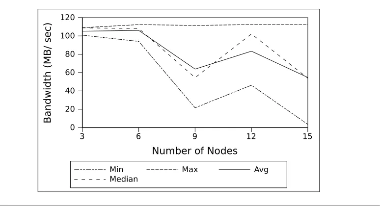
3 6 9 12 15 Number of Nodes
0 20 40 60 80 100 120
Bandwidth (MB/ sec)
Min Max Avg
Median
Figure 4.2: Network Performance for Parallel Workload on VCL Public interface
figure shows, the bandwidth of the system decreases with the addition of segments to the cluster. Since the number of segments which take part in the communication increases and the bandwidth of the system is bound to decrease.
Figure 4.3 displays the network bandwidth of the system for matrix workload when a cluster reservation of Greenplum with 3, 6, 9, 12 and 15 segments are reserved. As the figure shows, the bandwidth of the system decreases with the addition of segments to the cluster because of the increased communication intensity among all the segments. The decrease in effective bandwidth per segment due to matrix workload is higher than in the case of parallel workload since in matrix workload case communication takes place among the segments as well.
3 6 9 12 15
Number of Nodes
0 10 20 30 40 50 60
Bandwidth (MB/ sec)
Min Max Avg
Median
Figure 4.3: Network Performance for Matrix Workload on VCL Public interface
during your next reservation.
Results for the network bandwidth on private 10.x.x.x network was also taken with the same number of segments. The results observed were the same since the private network is also connected with 1Gig-E switch.
4.2
Validating I/O Performance
$ sudo /sbin/hdparm -tT /dev/sda /dev/sda:
Timing cached reads: 3400 MB in 2.00 seconds = 1699.34 MB/sec Timing buffered disk reads: 174 MB in 3.03 seconds = 57.38 MB/sec
However, since the machines are reserved in Cloud, users don’t have control in the actual I/O rate they want. It can change depending on the kind of hardware you receive during a reservation.
4.3
Storage Models
Greenplum provides heap or column oriented storage model depending on the kind of queries to be executed. OLTP transactions provides a better performance using heap storage model since insertion, deletion or updation on small number of rows takes place so it makes sense to store data in row-oriented format. On the other hand, OLAP transactions which are field oriented have fewer fetches from the disk if data is stored in column-oriented format.
Since the amount of data to be stored is huge ranging in terabytes or even petabytes, Greenplum also allows two kinds of compression which could be done on data, Quicklz and Zlib. There are 9 compression levels for Zlib if higher compression ration is desired. However, greater the compression ratio greater would be the time to execute the queries as well.
Table 4.1: Loading and Execution Times
Storage model Compression Loading time Execution time Heap None 16m 50.07s 3m 20.221s Column None 14m 16.63s 2m 36.578s Column Quicklz 13m 44.82s 2m 50.788s Column ZLib level= 5 13m 38.94s 2m 51.065s
Greenplum is optimized for Data Warehousing where desired storage model is Column-oriented, time taken to store data using Heap storage model is higher compared to time taken using Column storage model. Moreover loading time decreases as if compression is applied. However, if the compression time is more than the time taken to load the data, these time may be higher in some cases depending on the configuration of the machines as well. Column oriented storage model with no compression gives the best execution time, since there is no overhead in decompressing the data which is fetched from the database. Time taken for heap storage model is high because TPC-H benchmark is used which is suitable benchmark for OLAP type queries where Column-oriented storage model is desired too.
4.4
Performance Analysis
1 3 6 9 12 15 Number of Nodes
0 200 400 600 800 1000
Time in Seconds
Execution Time Load COPY
load GPLOAD
Figure 4.4: Loading and Execution Time on different Cluster Size
which were used as Extract Transform Load(ETL) servers from where data was loading in the machines. Loading was performed in two ways. The first method used COPY command provided by PostgreSQL which loaded the data from Greenplum Master to respective segments. The second method used GPLOAD command which loaded data from ETL servers into the cluster to utilize parallel loading feature provided by Greenplum. However, using gpload data could only be loaded using public network interfaces, so the private network interface in Configuration 2 and 3 was not utilized since they were not accessible from machines outside the cluster. For more information on gpload, refer to Greenplum’s Administrative Guide[14]. Some of the analysis are described below. To get the exact reading please refer to Appendix C and to see the individual execution time of all the queries executed refer to Table D.9.
Config 1 Config 2 Config 3 Type Of Configuration
0 50 100 150 200 250 300 350 400 450
Time in Seconds
Execution Time Load COPY load GPLOAD
Figure 4.5: Loading and Execution Time on different Configuration
network interfaces and contains only the primary segment. As observed, with the increase in number of segments, execution time of the Benchmark decreases by a considerable time. Loading time using GPLOAD is higher compared to COPY command with smaller nodes because of the initial time taken to create external tables and to start gpfdist on the machines. Moreover it is utilizing only one network interface while COPY command utilized both network interfaces. But as the number of nodes increase, time taken using GPLOAD rapidly decreases because of its parallel loading features. It however becomes constant at one point on reaching the maximum parallelism it can perform. The ETL servers has a data reading rate of 30 MB/sec so while using 2 ETL serves, the maximum bandwidth achieved is around 57MB/sec.
configuration 2 since only one network interface is used. Between configuration 2 and 3, loading time for configuration 3 is higher because data needs to be mirrored as well. By using GPLOAD command to load data, time remains constant almost in all the configuration because only one network interface is used between all the configurations, but the overall loading time is less than using COPY command stating Greenplum’s loading feature is faster. Time taken to execute TPCH benchmark is reduced by a factor of 2 between configuration 1 and 2 because of addition of one more network interface allowing faster data movement. The execution time remains same between configuration 2 and 3 since the same data is used.
CHAPTER
5
Conclusion and Future Work
5.1
Conclusion
This thesis is concerned with an assessment of the capabilities and issues that arise when an a high-performance data base intended for high-end analytics work is instantiated in a general purpose cloud environment. In this case, the environment was NC States VCL-gp cloud, and the data base was Greenplum.
re-sults since general cloud environments typically are not designed to deliver HPC/HPD performance. VCL is in some sense an exception since it does cater to both GP and HPC applications but the user needs to explicitely map an application on to appropriate hardware and topology.
Our experiments confirm that operation of Greenplum in a VCL-gp environment tends to be limited by the computational, networking and storage infrastructure on which Greenplum operates. When it operates on adequate infrastructure and when it is properly configured it outperforms many other solutions[3]. However, when its software-only solution is used in a typical VCL-gp cloud setting, the character of the provisioned hardware plays a major role. These results are presented in this thesis. In addition, we observe that it does take considerable expertise to tune Greenplum in a VCL-gp environment.
5.2
Future Work
REFERENCES
[1] A special report on managing information: Data, data everywhere. The Economist, February 2010. URL: http://www.economist.com/node/15557443.
[2] Hector Garcia-Molina. Database Systems : The Complete Book. Pearson Prentice Hall, Upper Saddle River, N.J., 2nd edition, 2009.
[3] EMC. Greenplum database: Critical mass innovation. Architecture White Paper, August 2010. URL: http://www.emc.com/collateral/hardware/white-papers/
h8072-greenplum-database-wp.pdf.
[4] EMC. Pursuing the agile enterprise: How a unified analytics strategy can drive business value. Greenplum UAP White Paper, 2012. URL: http://www.greenplum.
com/sites/default/files/UAP_whitepaper_0.pdf.
[5] Teradata. Teradata solution technical overview. Architecture White Paper, July 2012. URL: http://www.teradata.com/brochures/
Teradata-Solution-Technical-Overview-eb3025/.
[6] Oracle. A technical overview of oracle exadata database ma-chine and exadata storage server, January 2012. URL: http://www. oracle.com/technetwork/server-storage/engineered-systems/exadata/
exadata-technical-whitepaper-134575.pdf.
[7] Aster Systems Data Inc. A revolutionary approach for advanced analytics and big data management. Architecture White Paper, 2011. URL: http://www.asterdata.
com/wp_Aster_Data_Applications_Within/index.php?ref=rhs.
[8] TPC BENCHMARK H. Transaction Processing Performance Council (TPC), San Francisco, CA, 2.8.0 edition, September 2008. URL: http://www.tpc.org/tpch/
spec/tpch2.8.0.pdf.
[9] H.E. Schaffer, S.F. Averitt, M.I. Hoit, A. Peeler, E.D. Sills, and M.A. Vouk. Ncsu’s virtual computing lab: A cloud computing solution. Computer, 42(7):94 –97, july 2009. ISSN 0018-9162. doi: 10.1109/MC.2009.230.
[11] VCL. How do i get started. General Information, March 2012. URL: http://vcl.
ncsu.edu/help/general-information/how-do-i-get-started.
[12] Borko Furht. Handbook of Cloud Computing. Springer, New York, September 2010. ISBN 9781441965233.
[13] EMC. Greenplum Database 4.1 Installation Guide, a02 edition, 2010. URL: http://media.gpadmin.me/wp-content/uploads/2011/02/GPInstallGuide-4.
0.4.0.pdf.
[14] EMC. Greenplum Database 4.1- Administrator Guide, a03 edition, 2011. URL:http:
//media.gpadmin.me/wp-content/uploads/2011/05/GP-4100-AdminGuide.pdf.
[15] Marcus Collins. Hadoop and mapreduce: Big data analytics. Gartner burton it1 research note g00208798, Gartner, January 2011. URL:http://www.gartner.com/
id=1521016.
[16] EMC. Advanced cyber analytics with greenplum database. White Paper, July 2011. URL: http://www.greenplum.com/sites/default/files/EMC_Greenplum_
Adv%20Cyber%20Analytics_WP.pdf.
APPENDIX
A
Loading and Testing Scripts
There were two important scripts which were written for the configuring of Greenplum and to run loading and execution tests on the configuration:
A.1
/etc/init.d/vcl post reserve
The following is the script which is to be written in /etc/init.d/vcl post reserve and is executed as root by the management node. This script has two parts. The first part is to be written in every machine, the segments and the master node. The second part is written only in the master node.
# Configure external ssh
mv -f ./temp /etc/ssh/external sshd config
sed ’s/PermitRootLogin no/PermitRootLogin yes/’</etc/ssh/external sshd config>temp mv -f temp /etc/ssh/external sshd config
sed ’s/#PermitEmptyPasswords no/PermitEmptyPasswords yes/’ </etc/ssh/external -sshd config>/etc/ssh/temp
mv -f /etc/ssh/temp /etc/ssh/external sshd config /etc/rc.d/init.d/ext sshd stop
sleep 2
/etc/rc.d/init.d/ext sshd start
# Configure Internal ssh
sed ’s/AllowUsers .*/AllowUsers */’</etc/ssh/sshd config >/etc/ssh/temp mv -f /etc/ssh/temp /etc/ssh/sshd config
sed ’s/PermitRootLogin no/PermitRootLogin yes/’</etc/ssh/sshd config>/etc/ssh/temp mv -f /etc/ssh/temp /etc/ssh/sshd config
sed ’s/#PermitEmptyPasswords no/PermitEmptyPasswords yes/’ </etc/ssh/sshd config >/etc/ssh/temp
mv -f /etc/ssh/temp /etc/ssh/sshd config /etc/rc.d/init.d/sshd stop
sleep 2
/etc/rc.d/init.d/sshd start
## Copy the RSA keys to the root ssh files to ssh without password cp /home/gpadmin/.ssh/id rsa /root/.ssh/
cat /home/gpadmin/.ssh/authorized keys >>/root/.ssh/authorized keys
## Stop the firewall /etc/init.d/iptables stop
## Change the read ahead value /sbin/blockdev –setra 16384 /dev/sda
## Add gpadmin to the list of sudoers chmod 640 /etc/sudoers
echo gpadmin ALL= NOPASSWD: ALL>>/etc/sudoers chmod 440 /etc/sudoers
The following part is to be appended only in the master node.
## Create the files required for initializing greenplum
while read line; do
line=$(echo $line |tr -d ” ”)
values=$(echo $line |tr ”=” ”\n\\”) if [[ $values == *parent* ]]
then
set – $values
IP0=$(/sbin/ifconfig eth0 |grep inet |awk ’print $2’ |awk -F: ’print $2’) IP1=$2
echo $mhname>>/usr/local/greenplum-db/hostfiles/hostfile exkeys echo $IP0 >>/usr/local/greenplum-db/hostfiles/hostfile exkeys echo $IP1 >>/usr/local/greenplum-db/hostfiles/hostfile exkeys fi
done <”/etc/cluster info”
rm -f /usr/local/greenplum-db/hostfiles/hostfile gpinitsystem rm -f /usr/local/greenplum-db/hostfiles/hostfile gpssh segonly
while read line; do
line=$(echo $line |tr -d ” ”)
values=$(echo $line |tr ”=” ”\n\\”) if [[ $values == *child* ]]
then
set – $values IP1=$2
IP0=$(ssh -n $IP1 ifconfig eth0 |grep inet |awk ’print $2’ |awk -F: ’print $2’) hname=$(ssh -n $IP1 hostname)
echo $hname >>/usr/local/greenplum-db/hostfiles/hostfile exkeys
echo $hname >>/usr/local/greenplum-db/hostfiles/hostfile gpssh segonly echo $IP0 >>/usr/local/greenplum-db/hostfiles/hostfile exkeys
echo $IP1 >>/usr/local/greenplum-db/hostfiles/hostfile exkeys echo $IP0 >>/usr/local/greenplum-db/hostfiles/hostfile gpinitsystem echo $IP1 $hname>>/etc/hosts
fi
## Change the ownership of greenplum files to user gpadmin
chown gpadmin /usr/local/greenplum-db/hostfiles/hostfile gpinitsystem chown gpadmin /usr/local/greenplum-db/hostfiles/hostfile gpssh segonly chown gpadmin /usr/local/greenplum-db/hostfiles/gpinitsystem config
## Configure and Start Greenplum as user ’gpadmin’ cd /home/gpadmin/
su gpadmin -c ’gpinitsystem -c /usr/local/greenplum-db/hostfiles/gpinitsystem config’
A.2
testScript.sh
This scripts is placed in the directory of TPCH benchmark and is executed after generating the data and queries which needs to be executed using dbgen and qgen programs provided by the benchmark.
runCmd() {
COMMAND=”$1” declare RETVAL
printf ”\nRunning command \”%s\” ...” ”$COMMAND” bash -l -c ”$COMMAND” >& sysout
RETVAL=$?
if [ $RETVAL -ne 0 ]; then
printf ”\nError running command %s\nExiting...\n” ”$COMMAND” printf ”\nOutput is in file %s\n” ‘pwd‘/sysout
printf ”done.\n” rm -f sysout fi
}
export PGDATABASE=lukelonergan hostname=$(hostname)
for i in 1g 10g 20g do
for j in 1 2 3 4 do
printf ”==========================>Test Data $j\n” cp -f ./dss$j.ddl ./dss.ddl
runCmd ”psql -d postgres -c ’drop database if exists $PGDATABASE’” runCmd ”createdb $PGDATABASE -E UTF8”
runCmd ”psql -f dss.ddl” totTime=0
for file in nation.yml region.yml part.yml supplier.yml partsupp.yml customer.yml orders.yml lineitem.yml
do
sed ”s/HOST:.*/HOST: $hostname/” ./yml/$i/$file>temp.yml t=$(gpload -f temp.yml |grep seconds |cut -f4 -d’ ’)
printf ’Loading table... %s\t %f\n’ $file $t done
printf ’\n\n\n\n’ done
done
APPENDIX
B
Run Time Instances
This appendix will give a layout of the machines when cluster of 3 images were reserved, 1 Master and 2 Greenplum segments. The environment and performance may change because the instances you receive in cloud may change. Below are some of the features observed in this reservation.
• /etc/cluster info parent= 152.46.17.99 child= 152.46.16.240 child= 152.46.18.119
• /usr/local/greenplum-db/hostfiles/hostfile exkeys bn17-99.dcs.mcnc.org
152.46.17.99
bn16-240.dcs.mcnc.org 10.25.2.213
152.46.16.240
bn18-119.dcs.mcnc.org 10.25.2.214
152.46.18.119
• /usr/local/greenplum-db/hostfiles/hostfile gpinitsystem 10.25.2.213
152.46.16.240 10.25.2.214 152.46.18.119
• /usr/local/greenplum-db/hostfiles/hostfile gpssh segonly bn16-240.dcs.mcnc.org
bn18-119.dcs.mcnc.org
• Network Layout: Figure B.1 displays the layout of the machines reserved. As observed, the machines were reserved on the bus so that they can communicate with each other without reaching the switch. The public IP addresses are given by the the DHCP server and the private IP addresses are managed by the management node.
Network Bus
Greenplum Segment 152.46.16.240
10.25.2.213
Greenplum Segment 152.46.18.119
10.25.2.214 Greenplum Master
152.46.17.99 10.25.2.191
Figure B.1: Machine Layout with with 2 Greenplum Segments
$ /sbin/arp
Address HWtype Hwaddress Flags Iface 10.25.2.213 ether 00:14:5E:BE:39:24 C eth0 bn18-119.dcs.mcnc.org ether 00:14:5E:BE:39:B1 C eth1 bn16-240.dcs.mcnc.org ether 00:14:5E:BE:39:25 C eth1 10.25.2.214 ether 00:14:5E:BE:39:B0 C eth0
• PING Results: ping command was used between machines to check delay in com-munication between two machines. The results are as follows:
$ ping 152.46.16.240
— 152.46.16.240 ping statistics —
3 packets transmitted, 3 received, 0% packet loss, time 2000ms rtt min/avg/max/mdev = 0.124/0.140/0.168/0.023 ms
$ ping 152.46.18.119
PING 152.46.18.119 (152.46.18.119) 56(84) bytes of data. 64 bytes from 152.46.18.119: icmp seq=1 ttl=64 time=0.143 ms 64 bytes from 152.46.18.119: icmp seq=2 ttl=64 time=0.121 ms 64 bytes from 152.46.18.119: icmp seq=3 ttl=64 time=0.119 ms — 152.46.18.119 ping statistics —
APPENDIX
C
Results obtained from Greenplum Images
C.1
Loading and Execution Results
Results were taken with 3 different configurations. To know the detail of each configuration refer to Section 3.4. Tests to calculate the loading time and execution time for 1, 10 and 20 GB of data was calculated on running the benchmark on Greenplum cluster images with 1, 3, 6, 9, 12 and 15 segments. The results of the test may vary sometimes depending on the type of machine reserved and the network interface received on the images. Tables C.1, C.2 and C.3 below depicts the results obtained. The units for LD COPY, LD GPLOAD and execution time is in seconds.
Table C.1: Loading and Execution Times for Configuration 1
Nodes Data Storage Compression LD COPY LD GPLOAD Exec time
1
1 GB
Heap None 276 NA 158
Column
None 75 NA 139
Quicklz 78 NA 165
ZLib(5) 140 NA 164
10 GB
Heap None 2495 NA 7546
Column
None 908 NA 1833
Quicklz 923 NA 1805
ZLib(5) 1461 NA 1803
3
1 GB
Heap None 105 127 57
Column
None 33 72 49
Quicklz 31 68 60
ZLib(5) 49 84 58
10 GB
Heap None 1046 1095 1302
Column
None 402 572 512
Quicklz 405 513 582
ZLib(5) 508 710 590
20 GB
Heap None 2174 2321 4961
Column
None 860 1083 1171
Quicklz 854 1008 1197
ZLib(5) 1005 1346 1196
6
1 GB
Heap None 52 79 33
Column
None 31 45 29
Quicklz 28 45 33
ZLib(5) 31 50 33
10 GB
Heap None 672 623 288
Column
None 354 240 255
Quicklz 389 237 297
ZLib(5) 395 267 293
20 GB
Heap None 1399 1377 1280
Column
None 849 536 540
Quicklz 832 432 602
ZLib(5) 829 501 609
9
1 GB
Heap None 40 55 24
Column
None 29 35 22
Quicklz 31 35 25
ZLib(5) 30 38 25
10 GB
Heap None 602 465 193
Column
None 380 195 173
Table C.1 Continued
Nodes Data Storage Compression LD COPY LD GPLOAD Exec time
9 20 GB
Heap None 1241 858 410
Column
None 934 358 348
Quicklz 924 365 404
ZLib(5) 896 421 402
12
1 GB
Heap None 35 48 19
Column
None 30 35 17
Quicklz 30 31 20
ZLib(5) 30 32 20
10 GB
Heap None 555 422 148
Column
None 378 205 130
Quicklz 436 186 151
ZLib(5) 463 184 152
20 GB
Heap None 1090 742 297
Column
None 924 361 266
Quicklz 915 347 306
ZLib(5) 894 351 308
15
1 GB
Heap None 35 40 16
Column
None 31 31 14
Quicklz 30 30 16
ZLib(5) 32 31 16
10 GB
Heap None 557 361 120
Column
None 378 186 109
Quicklz 407 179 129
ZLib(5) 394 179 125
20 GB
Heap None 1009 612 238
Column
None 830 339 279
Quicklz 807 335 247
ZLib(5) 789 332 250
Table C.2: Loading and Execution Times for Configuration 2
Nodes Data Storage Compression LD COPY LD GPLOAD Exec time
1 1 GB
Heap None 163 275 88
Column
None 44 98 77
Quicklz 43 95 91
Table C.2 Continued
Nodes Data Storage Compression LD COPY LD GPLOAD Exec time
1 10 GB
Heap None 1504 2281 5840
Column
None 459 954 1049
Quicklz 450 807 960
ZLib(5) 732 1085 946
3
1 GB
Heap None 67 131 33
Column
None 28 60 31
Quicklz 32 57 32
ZLib(5) 33 65 32
10 GB
Heap None 794 1018 1299
Column
None 371 399 301
Quicklz 386 293 325
ZLib(5) 408 395 335
20 GB
Heap None 1591 1954 4833
Column
None 853 715 695
Quicklz 815 536 690
ZLib(5) 803 774 675
6
1 GB
Heap None 43 56 19
Column
None 32 39 17
Quicklz 33 37 20
ZLib(5) 34 41 19
10 GB
Heap None 594 469 179
Column
None 351 214 142
Quicklz 340 194 165
ZLib(5) 318 206 165
20 GB
Heap None 1281 981 1263
Column
None 786 490 326
Quicklz 819 375 348*
ZLib(5) 814 382 345
9
1 GB
Heap None 42 56 13
Column
None 33 40 12
Quicklz 32 35 14
ZLib(5) 34 39 14
10 GB
Heap None 594 408 109
Column
None 372 197 90
Quicklz 413 184 129
ZLib(5) 410 184 124
20 GB
Heap None 1087 714 252
Column
None 854 371 206
Quicklz 847 347 219
Table C.2 Continued
Nodes Data Storage Compression LD COPY LD GPLOAD Exec time
12
1 GB
Heap None 42 53 11
Column
None 32 37 10
Quicklz 34 35 11
ZLib(5) 33 36 11
10 GB
Heap None 520 298 86
Column
None 379 181 78
Quicklz 445 179 87
ZLib(5) 421 180 86
20 GB
Heap None 1006 546 167
Column
None 864 346 142
Quicklz 889 344 164
ZLib(5) 895 339 176
15
1 GB
Heap None 41 50 11
Column
None 32 36 10
Quicklz 32 34 10
ZLib(5) 34 34 10
10 GB
Heap None 488 270 71
Column
None 361 180 65
Quicklz 406 179 72
ZLib(5) 408 179 73
20 GB
Heap None 943 506 137
Column
None 825 347 126
Quicklz 820 341 137
ZLib(5) 814 331 138
Table C.3: Loading and Execution Times for Configuration 3
Nodes Data Storage Compression LD COPY LD GPLOAD Exec time
1 1 GB
Heap None 270 NA 102
Column
None 55 NA 78
Quicklz 47 NA 91
ZLib(5) 77 NA 91
3
1 GB
Heap None 91 148 38
Column
None 35 81 32
Quicklz 33 75 37
Table C.3 Continued
Nodes Data Storage Compression LD COPY LD GPLOAD Exec time
3
10 GB
Heap None 1019 1249 1395
Column
None 406 397 301
Quicklz 456 310 322
ZLib(5) 455 431 324
20 GB
Heap None 2030 2560 3834
Column
None 934 817 696
Quicklz 901 628 670
ZLib(5) 883 815 658
6
1 GB
Heap None 58 94 19
Column
None 35 52 18
Quicklz 34 48 21
ZLib(5) 35 50 20
10 GB
Heap None 747 797 190
Column
None 395 236 168
Quicklz 415 202 168
ZLib(5) 409 220 169
20 GB
Heap None 1440 1382 1932
Column
None 972 483 322
Quicklz 949 381 340
ZLib(5) 928 410 339
9
1 GB
Heap None 54 55 13
Column
None 34 48 12
Quicklz 34 42 14
ZLib(5) 34 45 14
10 GB
Heap None 656 471 134
Column
None 413 188 114
Quicklz 473 194 116
ZLib(5) 464 189 119
20 GB
Heap None 1107 856 268
Column
None 961 420 202
Quicklz 933 349 232
ZLib(5) 912 348 229
12 1 GB
Heap None 50 64 12
Column
None 35 48 10
Quicklz 35 43 11
Table C.3 Continued
Nodes Data Storage Compression LD COPY LD GPLOAD Exec time
12
10 GB
Heap None 550 378 98
Column
None 357 190 81
Quicklz 391 190 90
ZLib(5) 408 179 92
20 GB
Heap None 1010 691 200
Column
None 857 353 156
Quicklz 825 342 171
ZLib(5) 819 341 171
Table C.4: Network Performance on Private Interface
Workload Nodes Min(MB/sec) Max(MB/sec) Avg(MB/sec) Median(MB/sec)
Serial
3 112.32 112.36 112.34 112.36
6 111.33 112.36 112.07 112.33
9 111.8 112.4 112.2 112.35
12 111.99 112.4 112.27 112.31
15 111.53 112.41 112.31 112.36
Parallel
3 54.91 107.97 81.95 107.61
6 112.31 112.37 112.34 112.36
9 21.99 111.63 64 58.36
12 11.63 112.38 68.75 83.19
15 4.57 112.42 76.57 111.58
Matrix
3 33.02 48.52 41.19 45.22
6 3.52 25.49 13.27 14.87
9 1.34 47.04 9.58 7.53
12 0.76 47.28 6.69 3.8
Table C.5: Network Performance Across Reservations
Nodes Workload Characteristics Reservation 1 Reservation 2 Reservation 3
3
Serial
Min 112.35 112.33 112.33
Max 112.36 112.37 112.41
Avg 112.36 112.35 112.36
Median 112.35 112.35 112.37
Parallel
Min 100.85 94.86 90.63
Max 109.01 98.14 98.51
Avg 105.18 96.22 94.59
Median 108.85 96.76 97.39
Matrix
Min 25.8 19.36 14.25
Max 45.18 60.34 53.78
Avg 34.38 37.56 32.05
Median 39.71 32.96 27.64
6
Serial
Min 110.22 112.32 112.35
Max 112.36 112.38 112.35
Avg 111.18 112.35 112.35
Median 110.94 112.36 112.35
Parallel
Min 94.01 84.15 25.39
Max 112.35 112.36 111.27
Avg 106.92 105.14 74.42
Median 108.08 108.94 86.95
Matrix
Min 2.01 3.94 2.71
Max 45.05 44.13 38.06
Avg 14.21 14.55 15.53
Median 9.11 15.4 18.82
9
Serial
Min 112.35 112.33 112.33
Max 112.38 112.4 112.4
Avg 112.36 112.36 112.36
Median 112.36 112.35 36.112
Parallel
Min 4.47 25.89 15.12
Max 112.39 100.65 112.35
Avg 88.69 58.53 87.86
Median 112.21 56.09 109.3
Matrix
Min 2.16 1.82 2.1
Max 37.82 36.49 39.87
Avg 9.28 9.03 10.1
Table C.5 Continued
Nodes Workload Characteristics Reservation 1 Reservation 2 Reservation 3
12
Serial
Min 112.34 112.35 112.33
Max 112.42 112.41 112.41
Avg 112.37 112.36 112.36
Median 112.36 112.25 112.35
Parallel
Min 28.55 41.95 11.02
Max 112.42 112.41 70.02
Avg 67.59 69.5 37.27
Median 61.48 56.28 36.49
Matrix
Min 1.11 1.28 0.68
Max 35.26 39.05 53.42
Avg 7.16 6.92 6.47
Median 3.62 3.24 4.03
15
Serial
Min 88.4 112.26 110.83
Max 112.36 112.4 112.37
Avg 106.11 112.35 112.23
Median 109.63 112.35 112.35
Parallel
Min 3.54 5.09 6.71
Max 112.25 105.08 112.41
Avg 54.65 39.08 56.13
Median 53.94 28.37 55.15
Matrix
Min 0.61 0.44 0.54
Max 41.03 43.65 50.74
Avg 5.59 5.09 5.07
APPENDIX
D
Specifications of TPC-H Benchmark
The following are the structure for the tables used by TPC-H benchmark. It generates data for 8 tables namely Part, Supplier, PartSupp, Orders, Lineitem, Customers, Region and Nation. The layout of all the tables are depicted below:
Table D.1: PART Table Layout
Column Name Datatype Requirement Comments P PARTKEY identifier Primary Key P NAME variable text, size 55
P MFGR variable text, size 25 P BRAND fixed text, size 10 P TYPE variable text, size 25
P size integer
P CONTAINER fixed text, size 10 P RETAILPRICE decimal
Table D.2: SUPPLIER Table Layout Column Name Datatype Requirement Comments S SUPPKEY identifier Primary Key S NAME fixed text, size 25
S ADDRESS variable text, size 40
S NATIONKEY Identifier Foreign Key to N NATIONKEY S PHONE fixed text, size 15
S ACCTBAL decimal
S COMMENT variable text, size 101
Table D.3: PARTSUPP Table Layout Column Name Datatype Requirement Comments
PS PARTKEY Identifier Foreign Key to P PARTKEY PS SUPPKEY Identifier Foreign Key to S SUPPKEY PS AVAILQTY integer
PS SUPPLYCOST Decimal
PS COMMENT variable text, size 199
Table D.4: CUSTOMER Table Layout Column Name Datatype Requirement Comments C CUSTKEY Identifier Primary Key C NAME variable text, size 25
C ADDRESS variable text, size 40
C NATIONKEY Identifier Foreign Key to N NATIONKEY C PHONE fixed text, size 15
C ACCTBAL Decimal
C MKTSEGMENT fixed text, size 10 C COMMENT variable text, size 117
Table D.5: NATION Table Layout Column Name Datatype Requirement Comments N NATIONKEY identifier Primary Key N NAME fixed text, size 25
Table D.6: ORDERS Table Layout Column Name Datatype Requirement Comments O ORDERKEY Identifier Primary Key
O CUSTKEY Identifier Foreign Key to C CUSTKEY O ORDERSTATUS fixed text, size 1
O TOTALPRICE Decimal O ORDERDATE Date
O ORDERPRIORITY fixed text, size 15 O CLERK fixed text, size 15 O SHIPPRIORITY Integer
O COMMENT variable text, size 79
Table D.7: LINEITEM Table Layout Column Name Datatype Requirement Comments
L ORDERKEY identifier Foreign Key to O ORDERKEY L PARTKEY identifier Foreign key to P PARTKEY L SUPPKEY Identifier Foreign key to S SUPPKEY L LINENUMBER integer
L QUANTITY decimal L EXTENDEDPRICE decimal L DISCOUNT decimal
L TAX decimal
L RETURNFLAG fixed text, size 1 L LINESTATUS fixed text, size 1 L SHIPDATE date
L COMMITDATE date L RECEIPTDATE date
L SHIPINSTRUCT fixed text, size 25
Table D.8: REGION Table Layout
Column Name Datatype Requirement Comments R REGIONKEY identifier Primary Key R NAME fixed text, size 25
There is a total of 22 queries which gets executed in TPC-H Benchmark. To get the full syntax of TPC benchmark queries, refer to the TPC H Benchmark manual[8]. The following are high level meaning of the queries which are executed:
• Pricing Summary Report Query(1):This query reports the amount of business that was billed, shipped, and returned.
• Minimum Cost Supplier Query(2): This query finds which supplier should be selected to place an order for a given part in a given region.
• Shipping Priority Query(3): This query retrieves the 10 unshipped orders with the highest value.
• Order Priority Checking Query(4): This query determines how well the order priority system is working and gives an assessment of customer satisfaction.
• Local Supplier Volume Query(5): This query lists the revenue volume done through local suppliers.
• Forecasting Revenue Change Query(6): This query quantifies the amount of revenue increase that would have resulted from eliminating certain company-wide discounts in a given percentage range in a given year. Asking this type of ”what if” query can be used to look for ways to increase revenues.
• Volume Shipping Query(7): This query determines the value of goods shipped between certain nations to help in the re-negotiation of shipping contracts.
• Product Type Profit Measure Query(9): This query determines how much profit is made on a given line of parts, broken out by supplier nation and year.
• Returned Item Reporting Query(10): The query identifies customers who might be having problems with the parts that are shipped to them.
• Important Stock Identification Query(11): This query finds the most impor-tant subset of suppliers’ stock in a given nation.
• Shipping Modes and Order Priority Query(12): This query determines whether selecting less expensive modes of shipping is negatively affecting the critical-priority orders by causing more parts to be received by customers after the committed date.
• Customer Distribution Query(13): This query seeks relationships between customers and the size of their orders.
• Promotion Effect Query(14): This query monitors the market response to a promotion such as TV advertisements or a special campaign.
• Top Supplier Query(15): This query determines the top supplier so it can be rewarded, given more business, or identified for special recognition.
• Parts/Supplier Relationship Query(16): This query finds out how many sup-pliers can supply parts with given attributes. It might be used, for example, to determine whether there is a sufficient number of suppliers for heavily ordered parts.
of certain parts. This may reduce overhead expenses by concentrating sales on larger shipments.
• Large Volume Customer Query(18):The Large Volume Customer Query ranks customers based on their having placed a large quantity order. Large quantity orders are defined as those orders whose total quantity is above a certain level.
• Discounted Revenue Query(19): The Discounted Revenue Query reports the gross discounted revenue attributed to the sale of selected parts handled in a particular manner. This query is an example of code such as might be produced programmatically by a data mining tool.
• Potential Part Promotion Query(20): The Potential Part Promotion Query identifies suppliers in a particular nation having selected parts that may be candidates for a promotional offer.
• Suppliers Who Kept Orders Waiting Query(21):This query identifies certain suppliers who were not able to ship required parts in a timely manner.
• Global Sales Opportunity Query(22): The Global Sales Opportunity Query identifies geographies where there are customers who may be likely to make a purchase.
Table D.9: Execution Time of Individual Queries Query Number Execution Time(Seconds)
1 102.99
2 4.33
3 9.64
4 6.73
5 9.65
6 5.63
7 37.40
8 9.21
9 32.96
10 10.43
11 2.45
12 7.22
13 12.64
14 6.02
15 14.10
16 5.65
17 10.33
18 38.93
19 8.18
20 14.62
21 27.16
22 7.03