Preface: Focus on imaging methods in granular physics
Axelle Amon, Philip Born, Karen E. Daniels, Joshua A. Dijksman, Kai Huang, David Parker, Matthias Schröter, Ralf Stannarius, and Andreas Wierschem
Citation: Review of Scientific Instruments 88, 051701 (2017); doi: 10.1063/1.4983052
View online: http://dx.doi.org/10.1063/1.4983052
View Table of Contents: http://aip.scitation.org/toc/rsi/88/5
REVIEW OF SCIENTIFIC INSTRUMENTS88, 051701 (2017)
Preface: Focus on imaging methods in granular physics
Axelle Amon,1 Philip Born,2 Karen E. Daniels,3 Joshua A. Dijksman,4 Kai Huang,5
David Parker,6Matthias Schr¨oter,7Ralf Stannarius,8and Andreas Wierschem9 1Institut de Physique de Rennes, UMR UR1-CNRS 6251, Universit´e de Rennes 1, 35042 Rennes, France
2Institut f¨ur Materialphysik im Weltraum, Deutsches Zentrum f¨ur Luft- und Raumfahrt, 51170 Cologne, Germany
3Department of Physics, North Carolina State University, Raleigh, North Carolina 27695, USA
4Physical Chemistry and Soft Matter, Wageningen University and Research, Wageningen, The Netherlands
5Experimentalphysik V, Universit¨at Bayreuth, 95440 Bayreuth, Germany
6School of Physics and Astronomy, University of Birmingham, Birmingham B15 2TT, United Kingdom
7Institute for Multiscale Simulation, Friedrich-Alexander-Universit¨at Erlangen-N¨urnberg (FAU),
91052 Erlangen, Germany
8Institut f¨ur Experimentelle Physik, Otto-von-Guericke-Universit¨at, 39106 Magdeburg, Germany
9Institute of Fluid Mechanics, Friedrich-Alexander-Universit¨at Erlangen-N¨urnberg (FAU), 91058 Erlangen,
Germany
(Received 16 January 2017; accepted 7 April 2017; published online 25 May 2017)
[http://dx.doi.org/10.1063/1.4983052]
I. CURRENT CHALLENGES
To see a world in a grain of sand, and a heaven in a wild flower.
The poemAuguries of Innocenceby William Blake illus-trates one of the complexities of granular physics: Each grain of sand is unique1 and the entirety of particle-particle inter-actions in a sand pile is unpredictable.2 While walking on a
beach, one intermittently experiences the transition between a rigid, solid-like state and a fluid-like state. One leaves behind the stress loading history in the form of footprints.3,4Stepping
into the water, one recognizes the sediments are looser in com-parison to the partially wet sand on the beach and susceptible to the surrounding fluid flow, leading to sand ripples.5
Continuum descriptions based on empirical assumptions can successfully describe rapid flows and sufficiently dilute granular gases.6–8 However, continuum approaches fail to describe slow dense flows or critical behavior such as intermit-tent flows, jamming, and pattern formation.9,10These systems are governed by phenomena which are hard to model in con-tinuum descriptions: strong dissipation at the contacts between the grains due to friction,11inelastic deformation,12and cohe-sion,13etc. Moreover, the athermal nature of the system does
not allow for the use of statistical physics to connect the micro-scale to the macro-scale.
One of the major issues in modeling granular materials arises from the fact that what happens at the scale of a single grain can impact the response of the whole material. In static piles and dense flows, the distribution of stress is governed by force chains.14 Those force chains sensitively depend on the individual contacts between the grains, and the history of loading those contacts.15,16Consequently, local properties of the contacts, such as their typical orientation or the nature of the frictional contacts, can modify the mechanical behavior of the system. For example, anisotropy in the orientation of those contacts,17arising due to shear, can have a major impact on the macroscopic response.
On an intermediate scale between the size of the grains and the sample as a whole, it has been shown that the non-affine motion of the system, at the scale of clusters of
typically ten grains, plays a non-negligible role in the mechan-ical response of the system.18This non-affine motion seems to control numerous features of amorphous materials such as the thickness of shear bands19or the eddy-like structures in dense flows.18Several nonlocal effects have been observed, particu-larly in confined flows. For example, it has been demonstrated that shear bands generate mechanical noise even deep into the seemingly static phase.20,21
Therefore, it is of paramount importance for a descrip-tion of granular matter to be able to make observadescrip-tions on many length scales: from the grain or contact scale, through the mesoscopic effects such as nonlocality and shear banding, which appear on the∼10 grain scale, even up to the scale of a full sample that may contain billions of grains.
At the grain scale, there are two generic issues making it difficult to extract data with any imaging technique. First, our most advanced imaging technologies have been developed to act as extensions for our eyes, which operate in the visible spectrum. However, most granular materials are opaque in this range of wavelengths. Even if the particles were transparent, their refractive index would not generically match that of the most common interstitial fluids (air or water), leading to mul-tiple scattering. Second, a large volume of raw data is required to analyze a complete granular system: even just a simple sugar cube contains on the order of 105individual grains. To identify
the center of mass and orientation of each of these grains, it is necessary to identify its spatial extent using several thou-sand voxels (3D pixels). As a consequence, several gigabytes of data need to be collected to analyze a single static packing of grains. Moreover, trying to describe any kind of dynamics will compound the problem by requiring a sufficiently high frame rate to collect those data.
There are a number of ways to address the opacity issue, even with visible light. A common technique is to perform quasi-two-dimensional (Q2D) experiments, allowing the com-plete tracking of particle positions22,23as well as the
particle-particle interactions.24 Another option is to restrict the data
collection to the surface of the granular system, with the dis-advantage that bulk properties can differ significantly from the
behavior at the surface.25–30If the volume fraction of the par-ticles is sufficiently low, stereo-camera or volumetric methods can be used to capture three-dimensional (3D) dynamics.31–33
If the particles are optically transparent, there exist two addi-tional options. Where the interstitial liquid can be chosen freely, index matching provides a means to acquire 3D data.34
Alternatively, it is possible to embrace the multiple scatter-ing effects and use coherent light to gather information from the resulting speckle pattern.35 Finally, we can abandon the range of visible light entirely and instead use penetrating radi-ation to obtain the data from the bulk of the sample. A variety of such methods are extensively covered in this focus edi-tion, covering terahertz electromagnetic radiaedi-tion,36radar,37 positron emission,38nuclear magnetic resonance,39and X-ray tomography.40
Several solutions also exist for the data-bandwidth issue, which are common to the various methods. Limiting the anal-ysis to 2D or the surface of a 3D system is an effective way to decrease the number of particles under analysis, at the expense of ignoring the bulk behavior. To access the bulk, it is possi-ble to restrict the analysis to quasi-static systems in which the driving is stopped during each cycle to take a snapshot. This will reduce the necessary frame rate to zero, eliminating problems with bandwidth. Alternatively, the experiment can be constructed so that only a subset of tracer particles is visi-ble to the image acquisition system, or to take depth-averaged signals, in order to retain the dynamics.
The present focus issue mainly covers imaging with elec-tromagnetic waves. Nevertheless, acoustic waves can also be used to measure local velocities of particles in dilute flows41,42 or elastic properties of the effective medium for dense sys-tems.43A problem is that multiple scattering prevents spatial
resolution with acoustic waves in dense granular piles. Another difficulty when using acoustic waves is the intrusiveness of the probe that acts at the level of the contacts between the grains. This overview article, as well as the following focus issue on imaging granular particles, aims to provide guidance and orientation concerning the experimental techniques which help to face all these challenges.
II. ACQUIRING PARTICLE POSITIONS, ORIENTATIONS, AND SHAPES
To acquire particle positions, orientations, and shapes, a two-step process is necessary. First, an image is made of a particle and its immediate surroundings. Second, the required
particle information is extracted through data analysis of those images. For both steps, there are multiple methods to chose from (TableI); in this Focus Issue, we discuss both steps in some detail.
To image a particle, some contrast between the particle and its surrounding medium is required. The most obvious method to detect particles is to use the visible part of the elec-tromagnetic spectrum. In this range, it suffices to use standard cameras to obtain digital images of a collection of particles. The only difference between 2D and 3D imaging is whether each configuration is represented as a single 2D image or as a stack of 2D slices. Due to both absorption and scatter, however, the visible spectrum has limited penetration into most materials. Since the time of the first packing experiments by Bernal,45one solution has been to create 3D images by phys-ically disassembling the packing and taking an image at each step. This method is still used in the present day for sufficiently slow flows.46
To avoid such destructive methods, and considerably improve the data collection rate, modern experiments com-monly use transparent granular media. For optical transmission through a pile of transparent glass marbles, however, scatter remains a significant limitation in going deeper than a few par-ticles inward from the boundary. The solution is to reduce the scatter by immersing the solid particles in an index-matched medium. To obtain the necessary image contrast, at least one of the two phases must be stained with a fluorescent dye. Thus, by illuminating a cross section of the medium with a sheet of light (usually via a laser), the fluorescent response of the dyed material within the sheet is captured by the cam-era. By moving the light sheet with respect to the sample and recording a series of slices, a 3D image of the medium can be created.
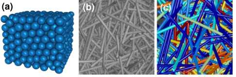
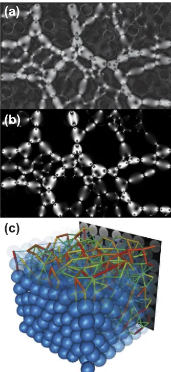
In the resulting 3D image, computerized-post process-ing algorithms can then be used to track particles, measure flow velocities, or identify shapes. This technique of Refrac-tive Index Matched Scanning (RIMS) has been covered by several review articles.47,48 The RIMS article in this Focus Issue will explore the application of RIMS34to hydrogel par-ticles in particular. These are soft elastic solids with a refractive index close to that of water. The softness of hydrogels provides a key feature: they deform significantly under modest loads. The presence of deformations at each contact makes it pos-sible to quantify individual contact forces on hydrogels, as is discussed in Sec.IV. The central challenge is to find the non-spherical contour of the particle. An example can be seen in Fig.1(a).
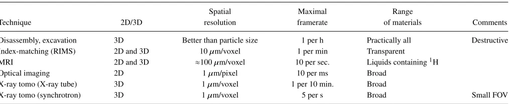
TABLE I. Techniques for obtaining particle coordinates, typical values.
Spatial Maximal Range
Technique 2D/3D resolution framerate of materials Comments
Disassembly, excavation 3D Better than particle size 1 per h Practically all Destructive Index-matching (RIMS) 2D and 3D 10µm/voxel 1 per min Transparent
MRI 2D and 3D ≈100µm/voxel 10 per sec. Liquids containing1H
Optical imaging 2D 1µm/pixel 10 per ms Broad
X-ray tomo (X-ray tube) 3D 1µm/voxel 1 per 10 min. Broad
051701-3 Amonet al. Rev. Sci. Instrum.88, 051701 (2017)
FIG. 1. 3D imaging of granular particles. (a) Compressed hydrogel spheres with 2 cm diameter (Educational Innovations), imaged by laser sheet scanning in an index-matched liquid. Particle deformations in a compressed packing of soft spheres are clearly visible, for example, in the flattening of spheres at the top. Such deformations are measurable at each particle-particle contact and yield information about contact forces. (b) Rendering of the volume data obtained by X-ray tomography, the particles are cylinders with 40 mm length and 1.4 mm diameter (Spaghettini Barilla N. 3). An animated version of similar raw data can be found at Ref.44. (c) Rendering of the same volume as in the last panel, but after the detection of all cylinder positions and orientations. The particles are color coded with their contact number. Images b and c by courtesy of Cyprian Lewandowski.
For non-transparent materials, Magnetic Resonance Imaging (MRI) can obtain contrast-rich images within the bulk.39MRI reveals the edges of particles by mapping the dis-tribution of NMR-active nuclei in liquids (or, in exceptional cases also in gases) within a sample. Two requirements have to be met. First, it is necessary to have a liquid constituent within the sample, since solids typically do not yield useful MRI signals. Second, the liquid needs to have NMR-active nuclei. There are a large number of NMR-active isotopes. While phos-phorus, fluorine, or13C enriched carbon would work in princi-ple, in practice all commercial MRI scanners work at the proton resonance frequency, i.e., they are tuned to detect the1H nuclei
in the sample. For this reason, the most common methods for achieving contrast are to use water- or oil-containing particles (e.g., seeds or synthetic capsules) or to coat/embed solid par-ticles in a hydrogen-containing fluid. In these cases, a conven-tional tomograph can achieve submillimeter spatial resolution. Samples of several dozen centimeters can be handled by large MRI tomographs, medical scanners, or wide-bore scanners.
Just as for RIMS, MRI can provide a 3D image or tomo-gramof a sample, from which particle orientations and shapes may be retrieved. In some situations, it suffices to record a single 2D slice of the sample in order to track the dynamics. If so, both RIMS and MRI can provide single slices at a faster data-collection rate (kHZ).
Another technique we discuss in this Focus Issue is X-ray tomography.40 Its advantages are superior spatial resolution
and the ability to work with a much more diverse set of mate-rials, including even pasta (see Figs.1(b)and1(c)). In contrast to visible light, X-rays will penetrate most granular samples with an intensity that decays exponentially with distance into the material. For a broad range of materials, the X-ray contrast is large enough to provide images. A major drawback is that the acquisition of even a simple cross-sectional view in general requires the same amount of time as the full 3D image. This makes the technique comparatively slow. A compromise is to take 2D transmission images (radiograms) by placing the gran-ular sample between an X-ray source and a camera equipped with a scintillator. In this case, the X-ray signal is integrated across the full sample.
In computed tomography (CT), a large number (typically
√
2 times the width of the image in pixels) of radiograms are collected while rotating the sample around an axis perpendicu-lar to the beam direction. From this sequence of images, a 3D representation of the sample is reconstructed using an algo-rithm called the inverse Radon transformation.49 Each voxel
represents the X-ray absorption coefficient within a volume element at the corresponding location in the sample. Since different materials have different absorption coefficients, this information can serve as the contrast to detect the boundaries of particles and thus allows identifying the position, shape, and orientation of all granular particles within the tomogram.40
The time needed to acquire an X-ray tomogram depends on the photon flux from the source. There are two types of sources: classical X-ray tubes and synchrotrons. X-ray tubes are comparatively low cost, allowing the production of turnkey, tabletop tomography setups with resolutions down to the sub-micron range. Such setups can even be assembled by scientists themselves.50However, X-ray tubes provide a low photon flux
and thus require 10 min to several hours to generate a sin-gle 3D image. Synchrotrons are several orders of magnitude brighter than X-ray tubes, thus allowing the acquisition of tomograms at rates up to several per second. However, because they are large user facilities, they require significant lead time starting with an application for beam time. Moreover, their field of view (FOV) is typically limited to less than a cubic centimeter.
All of the imaging methods discussed above provide a 2D or 3D image of a granular sample. The algorithmic anal-ysis steps required to quantify particle properties from such images are in principle generic and can in many cases be applied to images of any imaging method. However, since every imaging method comes with its own specific noise and artifacts, an algorithmic analysis of image data usually begins with a method-dependent step for denoising and removing artifacts.
Even with perfect image denoising and artifact removal, there remain significant fundamental challenges in image anal-ysis. A denoised image will be a 2D or 3D set of gray values. The gray value of each pixel/voxel can variously represent the amount of directly reflected light, the concentration of excited fluorescent dye, a density of spins, or an X-ray absorption coefficient. This could be measured for either the particle or for its surrounding medium. Either way, the number of pix-els/voxels is limited, and the gray values are drawn from a bounded set of integers. Thus, both the spatial resolution and the image contrast gradients are always finite. This limita-tion yields a fuzziness on the precise contour of every imaged particle. This is especially detrimental in images of dense par-ticulate media: the fuzziness limits our ability to recognize where particles are exactly located, whether two neighboring objects are touching, or even whether they are in fact separate entities.
addition, there are a number of post-processing methods to detect the location of a particle surface, for which the shape does not have to be knowna priori.34,51
After the extraction of detailed shape information about the location of the outer boundary of each particle, further analysis of the experimental data becomes possible. Com-mon techniques include examining nearest neighbor distribu-tions,40particle tracking and velocimetry (see Sec.III), contact force measurements (see Sec.IV), and more intricate measures that characterize the packing structure, such as Minkowski tensors.40
III. MEASURING PARTICLE DISPLACEMENTS AND VELOCITIES
Measuring velocities starts with first measuring the dis-placements of objects or patterns between two snapshots sepa-rated by a time interval. These measurements can then be accu-mulated into either a velocity field (for a Eulerian viewpoint) or particle-trajectories (Lagrangian viewpoint), according to the needs of the researcher.
In making displacement measurements, two fundamen-tal limitations must be considered. First, the precision with which the position of the objects is known, to be improved according to the techniques described in SectionII. Second, what choice of frame rate can be obtained using the chosen particle-finding method, and whether this time scale is suffi-ciently well-separated from the dynamics of interest. Several key sources of error inherent in these choices are reviewed in Ref.52.
The frame rate depends on parameters such as the desired resolution (number of pixels/voxels) and the exposure time needed for a sufficient signal-to-noise ratio. Depending on the specific questions of interest, different experimental strategies can be chosen. Innovative methods are often custom-designed for a particular situation. Performance indicators of the dif-ferent displacement/velocity methods discussed in this Focus Issue are summarized in TableII.
A straightforward method for obtaining the Lagrangian trajectories of well-identified particles is to start from a tem-poral sequence of their successive positions, and from these deduce their full velocities. High-precision particle position measurements play a key role in the success of this method, and identifying single particles is not trivial on its own. One way to track individual particles is to tag a small number of tracers
which can be easily distinguished. This can be done with either one or several cameras, to increase spatial or dimensional coverage. Tracking the centers of the particles is sufficient for studying translational motion. Rolling or sliding particle motion can be identified only by taking into account further characteristics of the extended particle, like form, intensity distribution, tracking marks or patterns on the particles, which will be discussed further in an article of this Focus Issue.53
For particles which are opaque or not index-matched with the surrounding media, velocity measurements are restricted to near-surface flows or to low particle concentra-tions. Refractive-index matching between fluid and particles allows the study of deeper layers in granular matter, a tech-nique discussed in one of the articles of the Focus Issue.34 Other techniques for tracking within the bulk include Positron Emission Particle Tracking (PEPT),38microwave radar
track-ing,37X-ray radiography,54or Magnetic Resonance Imaging
(MRI).39Tracer particles (single radioactively labeled in the
case of PEPT, high dielectric constant for radar tracking, steel spheres for X-ray radiography, or NMR-active nuclei for MRI) are then embedded inside the material (or spin-labeled in MRI) and the system is imaged while subjected to some excitation or loading. The knowledge of the complete trajectory of one or a few particles in 3D is then possible. In such methods, slow frame rates are not an impediment to the tracking of par-ticles as the parpar-ticles are well-separated in space. In the case of MRI, magnetization relaxation of labeled tracers may limit the total duration of the dynamics studied. Using PEPT38 a single particle can be followed almost indefinitely, and a well-mixed system can provide representative information on the entire phase space of this type of particle. In other systems, the trajectory of a single tracer is not always a representative of the whole velocity field, so that full-field methods are preferred.
In order to follow an assembly of indistinguishable grains, particle tracking velocimetry (PTV) can be achieved by matching particle positions across sequential images.55–57
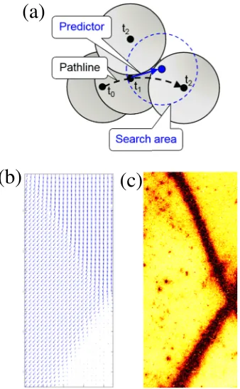
To discriminate identical particles in subsequent images, the displacement must be smaller than typically half of the spac-ing between particle centers, which requires that the frame rate is sufficiently large compared to the dynamics of the parti-cles.52For particle-matching between different frames, various algorithms can be employed. The principle behind tracking algorithms is shown in Figure2(a)and an example of a dis-placement field obtained using PTV is shown in Figure2(b). An important issue is obtaining sufficiently accurate positions
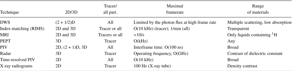
TABLE II. Techniques for obtaining particle velocities and displacements.
Tracer/ Maximal Range
Technique 2D/3D all part. framerate of materials
DWS (2 + 1/2)D All Limited by the photon flux at high frame rate Multiple scattering, low absorption Index-matching (RIMS) 2D and 3D Tracer or all O(10 kHz) (tracer); 1/min (all) Transparent
MRI 2D and 3D Tracers or all ≈10/s Only liquids containing1H
PEPT 3D Tracer O(kHz) Any
PIV 2D, (2 + 1)D, 3D All Interframe time: O(100 ns) Broad
Radar 3D Tracer Operating frequency, O(GHz) Contrast of dielectric constant
Time-resolved PIV 2D All O(10 kHz) Broad
051701-5 Amonet al. Rev. Sci. Instrum.88, 051701 (2017)
FIG. 2. (a) Sketch for particle matching in PTV using a predictor from previ-ous displacement. This method allows a more accurate tracking of the particles than a mere nearest-neighbor algorithm. The same displacement field obtained by two different methods ((b) and (c)) during a biaxial test after the failure of the material. (b) Displacement field obtained by tracking the reflection of the glass beads at the surface of the sample (PTV). (c) Deformation field obtained by computing correlation between two successive speckle images obtained from the coherent light backscattered by the material (DWS). Yellow: low deformation (.10−5), black: large deformation (&10−4). A description of the experiment and results can be found in Ref.35.
to identify displacements, while still operating at high enough frame to capture the dynamics. This trade-off is made dif-ferently for different systems. In general, 3D scans are used for studying slower dynamics, while fast dynamics require fast cameras aimed at a single slice of the material or a Q2D system. Where it is not possible to identify individual parti-cles, it is still possible to measure mean displacements (or velocity/deformation fields) using cross correlation techniques like particle image velocimetry (PIV).31–33These techniques work by subdividing individual frames into small interrogation areas. For these areas, the mean displacement is determined by cross correlation between subsequent frames. A sub-pixel resolution can be achieved by an appropriate choice of imag-ing conditions and the size of the interrogation area. Usimag-ing more than one camera, stereoscopic or volumetric studies can be carried out.
Two entirely different classes of methods allow the mea-surement of velocities without the step of identifying particles. The first is MRI, for which a useful variant utilizes a time-varying magnetic field as a probe. This allows the velocities of the MRI-active particles to be deconvolved from the response signal.58 The second class of methods is all based on the scattering of waves, as described next.
One variant of the second class is to identify the phase shift of the scattered wave with radio detection and rang-ing (radar) systems because it is determined by the relative
distance between the scatterer and the observer. Radar methods can be implemented using electromagnetic wavelengths from visible light (LIDAR) through microwave and radio waves (>10 m) depending on the applications.59Tracers with a good
contrast to the dielectric constant of the surrounding particles are then needed. For a moving target, a radar system com-pares the phase shift of the microwave being transmitted-to and scattered-from the object to get the position (moving tar-get indicator radar). Alternatively, it uses the Doppler effect to obtain the velocity (Doppler radar).60The main advantage of radar particle tracking is the good time resolution. For continuous wave radar systems, the time resolution is only limited by the analog-to-digital converter. Methods for using this technique to obtain the displacement and consequently the instantaneous velocity of a tracer are described in an article of this Focus Issue.37
The other variant is to embrace the multiple-scattering limit, which leads to a loss of the information contained in the propagating wave.36Terahertz methods are not yet capable of
measuring displacements or velocities. In the case of visible light and transparent grains, multiple scattering is unavoid-able. Nevertheless, for illumination using coherent light, rela-tive displacements can be obtained from the resulting speckle images arising from the interference of the numerous waves which have performed random walks in the system, a method called Diffusing-Wave Spectroscopy (DWS).61,62As with any interferometric method, minute relative displacements can be detected and typically deformations of the order of 105 can be obtained. In the case of back-scattering, most of the paths explore only a small volume in the vicinity of the illumi-nated plane. This means that spatially resolved displacement maps, with a resolution of typically a few bead diameters, can be obtained as a representation of the deformation field in a thin layer close to the plane of visualization. An example of a map of deformation obtained by this method is shown in Figure2(c). These techniques are reviewed in an article of this Focus Issue.35
Finally, as discussed in the introduction, acoustic echo42 or Doppler measurement41can be used to measure velocities in the limit of single scattering of the acoustic waves. The useful-ness of such methods is rapidly limited by multiple scattering in granular piles.63 Still, velocity fields have been recently obtained in dense suspensions using high-speed ultrasound imaging.64
IV. MEASURING INTER-PARTICLE FORCES
While rheological measurements67can provide the
FIG. 3. (a) Image of force chains obtained using darkfield photoelastic mea-surements in the setup described in Ref.65. The bright areas indicate the regions where contact forces modulate the photoelastic response of the disks. The quantitative extraction of contact forces works by finding the best set of contact forces to “fit” the bright pattern. (b) A computer generated fit to the data shown in (a). (c) Image of 3D interparticle forces obtained on frictionless hydrogel particles, from the experiment described in Ref.66.
not only particle positions but also interparticle forces. There-fore measuringforces between particlesbecomes necessary to completely understand particulate materials.
The requirement to measure forces between particles in such particulate materials presents the experimentalist with great challenges. While Debye theory can predict heat capac-ities by making simplifying assumptions about the number of modes in a crystal lattice and a Lennard-Jones interaction potential suffices to predict the elastic behavior of most solids, granular materials require a more detailed model. First, the interaction laws between particles are generically dissipative, hysteretic, rate dependent, and not pairwise additive.69,70 Sec-ond, the disordered nature eliminates the concept of linear response, such that “small deformation” analyses are of little use in understanding realistic materials.
Although it has been possible to obtain stress information at the boundary of a 3D system,71,72true understanding only comes if the spatiotemporal distribution of contact forces is also measured in the bulk of a particulate material, as it is often inhomogeneous and anisotropic. The complex distribution of
interparticle forces thus requires the experimentalist to mea-sure not only the already-complex interaction forces between particles but also their spatial structure in generally opaque or at highly scattering media. The daunting task of performing complex force measurements in the bulk of a particulate mate-rial was steadily solved by the work of successive generations of physicists and engineers.
Photoelasticity, the change of the polarization state of light due to the stresses inside a birefringent material, has a century-old history14,73,74of measuring stress and strain distributions within both solids and granular materials. However, until the pioneering work of Behringeret al.16in which both normal and tangential interparticle forces were first measured, photoelas-tic studies were limited to the study of stress fields, and not the interparticle contact forces themselves. The quantitative photoelastic method has evolved tremendously and is now in advanced development across multiple labs around the world. These modern, quantitative methods are described here in a Focus Issue article,24as well as in the original theses.75,76A
remaining challenge is that these methods are only suitable for Q2D studies if quantitative information is required.
Building on the development of conventional confocal microscopy tools, Brujicet al.77showed that it was possible to measure contact forces in the bulk of a 3D microemulsion (frictionless droplets) using fluorescent dyes. Since then, the emulsion measurement technique has grown to include a range of 3D force measurement techniques, including at larger gran-ular length scales for frictionless particles.66,78,79In all cases, the central challenge is to measure the size of the contacts, which proceeds using similar techniques to those described in SectionII. As described in a Focus Issue article,34such
mea-surements are now possible while simultaneously performing mechanical tests under realistic strains. Due to the experimen-tal and computational complexity of such studies, we present an overview of (partly published) experimental and compu-tational methods used in the study of packings of hydrogel spheres. Similarly, X-ray tomography of non-transparent, fric-tional particles can provide normal forces for sufficiently soft particles.80
In addition, several other techniques not covered by the Focus Issue deserve mention since they provide contact force measurements for hard, frictional particles for which defor-mations are not directly observable. Using a combination of x-diffraction and X-ray tomography, Hurleyet al.81have suc-cessfully measured inter-particle forces for a small sample of non-transparent particles under compression, and at the single-particle level. Chenet al.82have shown that it is possible to use
two-photon excitation to make pressure measurements within single ruby particles, based on shifts in the fluorescence spec-trum. It is an area of future research to use these methods to understand frictional responses through both the normal and tangential forces.
V. ACQUIRING OTHER PROPERTIES
051701-7 Amonet al. Rev. Sci. Instrum.88, 051701 (2017)
or structural measures. The analysis of large quantities of particles in order to calculate size distributions or pack-ing structures is limited by the generic issues discussed in Sec.I. When further investigations do not require positions and shapes of the individual particle, investigation methods directly sensitive to such intensive material properties can be an effective alternative. We restrict the discussion to methods which are used in the statistical physics analysis of granular media. Methods that were developed for process technologies like sieving or elutriation are beyond the scope of this Focus Issue.
A. Mean size and size distribution
The fundamental task is to provide a measurement of the spatial extent of the particles in the system. This can be done by imaging a sufficiently large number of particles, with sufficient resolution, using any of the methods listed in Sec. II. However, it may take an excessively long time to image the ensemble and process the data (separating, identi-fying, and fitting each one) using one of the imaging methods optimized for opaque 3D materials.40Specialized automated setups can image and process tens of thousands of particles in seconds, if disassembly of the sample andex situ character-ization of the particles are possible.83Particle sizes between a few micrometers and a few millimeters can be resolved by imaging.
An alternative to imaging is small-angle light scattering. This method relies on the multiple-scattering of light inten-sity by particles in a well-collimated light beam. The relative intensity changes are sensitive to the particle size, but only when the particles are not much larger than the wavelength of the light used. Consequently, specialized instruments are required to resolve the intensity changes by such scattering.84 Recently, terahertz radiation with 87µm wavelength has been applied to macroscopic granular particles, which has lowered the instrumental demands to a manageable range.85
In general, scattering methods can be applied to any par-ticle material. Mean parpar-ticle size and parpar-ticle size distribu-tions can be determined from single measurements on particle ensembles. Nonetheless, the samples must be disassembled
and heavily diluted in order to reach the independent-scattering regime. In practice, this leads to measurement times no faster than the automated imaging setups, and only radii of equiv-alent spheres are obtained.84Particles sizes between hundred
nanometers and roughly a millimeter can be analyzed with scattering.
B. Packing density and packing structure
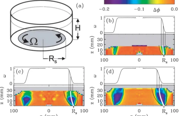
For some imaging methods which are sensitive to an extensive property of the sample, it is possible to use them in a way that reports the average packing density. For exam-ple, in X-ray radiography the intensity decreases exponentially with the number of particles in the beam path. Other exam-ples include index matching and MRI (compare Sec.II). For index-matched and fluorescent-dyed samples, the intensity of the signal is proportional to the number of particles containing fluorescence markers (or inversely proportional, if the liquid contains the fluorescence molecules). For MRI, the signal is proportional to the number of particles containing NMR-active liquids. This means that these methods can switch to a mode which records packing density, even when the resolution would be insufficient to resolve individual particles. In each case, the signal is normalized by a sample volume to obtain the packing density. These techniques have allowed X-ray radiograms to be used to study density variations in flowing sand,86,87
dila-tancy during fast shear,54,88,89or the formation of a jet after
a sphere impact into a granular medium.90,91MRI has been
further used to quantify the evolution of the local particle den-sity, e.g., in colloid transport,92during sedimentation,93–96or
in smooth granular shear97(see Fig.4).
Conventionally, methods that are directly sensitive to the packing structure rely on measuring scattering patterns. The scattering pattern is sensitive to the packing structure only for samples which exhibit single scattering of a certain wave.98 This is frequently the case for colloidal and atomic systems and light or X-ray scattering, but packing density and scatter-ing efficiency of granular media are too large for this technique to work.36One novel approach which moves the field towards direct structure sensitivity is presented in this Focus Issue. In Ref. 36, we show that the spectroscopic transmission of
terahertz radiation through granular materials reveals the posi-tion of the structure factor peak (the strongest correlaposi-tion length in the sample). This approach requires that the particle diameter is within the spectral range of the wavelengths used, and that the particle material does not absorb the radiation too much.
C. Particle contact stability
The local stability and the statistics of particle contacts in consolidated packings can be qualitatively probed with sound. Sound waves propagate within granular media along the force chains formed by the discrete particle contacts99and the
veloc-ity of the acoustic wave gives indication on the structure of the granular pile.100Scattering and dissipation of the wave occurs at each contact, leading to diffusive transmission of sound and high attenuation. Simulations have shown that the scattering losses are sensitive to the degree of disorder in the contact network.101 Intensity losses by dissipation are sensitive to friction at the contacts.43Time-of-flight measurements allow separating the contributions to attenuation by scattering and dissipation.43 The momentum and kinetic energy associated with the sound wave are often sufficient to induce rearrange-ments in granular media with low confining pressures, which can itself be used to probe rigidity and local unjamming in granular media.102,103Further investigations of the individual
contributions of dissipation, scattering, order, and mechanical impact by sound waves might lead to new methods to probe statistics of the contact network in granular media without having to image individual contacts.
VI. CONCLUSION AND OUTLOOK
This Focus Issue reviews methods for acquiring micro-scopic particle properties and for connecting them to the macroscopic physics of granular media. A variety of methods are presented, utilizing electromagnetic waves ranging fromγ -rays to radio waves. These methods provide information in the form of images, scattering, tomographic reconstruction, and the tracking of phase shifts. Each approach and probe has spe-cific demands on sample material, instrumental investments, and computational efforts and offers different sensitivities and spatiotemporal resolutions. This introductory article aims to assist the reader in selecting the most appropriate techniques for their particular research.
To consider the success of these methods, it is only neces-sary to return to the question raised in the initial paragraph of this paper: how do individual grains contribute to the intermit-tent flow of sand while walking on the beach? In spite of the latest advances in methods presented here, a comprehensive answer to such a question remains beyond reach of even the most advanced contemporary techniques.
As such, the methods presented here demand future devel-opments to improve both quality and precision. The contin-ued closing of the gap between the lab and beach can be deduced from the remaining limitations discussed in this paper. We expect most beneficial improvements will arise in the following area: (1) efficient tracking of both the translation (easier) and rotation (harder) of particles; (2) techniques for
investigating packings of irregular particles; (3) reconstructing 3D force distributions; (4) improved computational capabil-ity and efficiency. In particular, the simultaneous tracking of rotational motion of many particles is still in its infancy. Working with irregular particles may move studies away from the “spherical cow” paradigm towards more realistic sand grains. The development of low-cost 3D printers is already fostering rapid interest in more-complex shaped particles.104 Approaches to the reconstruction of forces in 3D packings of hard particles have been demonstrated by fluorescence imaging and X-ray diffraction.
Item (4) is particularly noteworthy, as it might seem that Moore’s law will take care of this problem without interfer-ence from granular scientists. However, each of the other three items on the list significantly increases the amount of data to be handled. Tracking rotation and translation at the same time doubles the amount of data per particle, working with irregular particles requires better shape detection algorithms and keep-ing track of more descriptive variables, and the reconstruction of 3D force distributions requires new detection and fitting algorithms as well as an increase in the number of parameters (contacts and force vectors) stored in the final dataset. As the spatiotemporal resolution of tomographic methods improves, the amount of data grows as a cubic function. As such, data science initiatives and algorithmic advances will be key to the success of the field.
1G. Greenberg,A Grain of Sand: Nature’s Secret Wonder(Voyageur Press, St. Paul, MN, 2008).
2J. Duran,Sands, Powders and Grains an Introduction to the Physics of
Granular Materials, 1st ed. (Springer-Verlag, New York, 2000). 3J. Geng, D. Howell, E. Longhi, R. P. Behringer, G. Reydellet, L. Vanel,
E. Cl´ement, and S. Luding, “Footprints in sand: The response of a granular material to local perturbations,”Phys. Rev. Lett.87, 035506 (2001). 4S. Herminghaus,Wet Granular Matter: A Truly Complex Fluid(World
Scientific, Singapore, 2013).
5F. Charru, B. Andreotti, and P. Claudin, “Sand ripples and dunes,”Annu.
Rev. Fluid Mech.45, 469–493 (2013).
6J. T. Jenkins and S. B. Savage, “A theory for the rapid flow of identical,
smooth, nearly elastic, spherical particles,”J. Fluid Mech.130, 187 (1983). 7I. Goldhirsch, “Rapid granular flows,”Annu. Rev. Fluid Mech.35, 267
(2003).
8G. D. R. MiDi, “On dense granular flows,”Eur. Phys. J. E14, 341 (2004).
9A. J. Liu and S. R. Nagel, “The jamming transition and the marginally
jammed solid,”Annu. Rev. Condens. Matter Phys.1, 347 (2010). 10I. S. Aranson and L. S. Tsimring,Granular Patterns(Oxford University
Press, 2009).
11S. Luding, “Granular materials under vibration: Simulations of rotating
spheres,”Phys. Rev. E52, 4442 (1995).
12N. Brilliantov and T. P¨oschel,Kinetic Theory of Granular Gases(Oxford University Press, Oxford, New York, 2004).
13T. M¨uller and K. Huang, “Influence of the liquid film thickness on the
coefficient of restitution for wet particles,”Phys. Rev. E93, 042904 (2016). 14P. Dantu, “Contribution l’´etude m´echanique et g´eom´etrique des milieux
pulv´erulents,” in Proceedings of the Fourth International Conference on Soil Mechanics and Foundation Engineering(Butterworths Scientific Publications, London, 1957), pp. 144–148.
15J. Geng, E. Longhi, R. Behringer, and D. Howell, “Memory in
two-dimensional heap experiments,”Phys. Rev. E64, 060301 (2001). 16T. S. Majmudar and R. P. Behringer, “Contact force measurements and
stress-induced anisotropy in granular materials,”Nature435, 1079–1082 (2005).
17F. Radjai, D. E. Wolf, M. Jean, and J.-J. Moreau, “Bimodal character
of stress transmission in granular packings,”Phys. Rev. Lett.80, 61–64 (1998).
18F. Radjai and S. Roux, “Turbulentlike fluctuations in quasistatic flow of
051701-9 Amonet al. Rev. Sci. Instrum.88, 051701 (2017)
19P. Schall and M. van Hecke, “Shear bands in matter with granularity,”
Annu. Rev. Fluid Mech.42, 67–88 (2010).
20K. Nichol, A. Zanin, R. Bastien, E. Wandersman, and M. van Hecke,
“Flow-induced agitations create a granular fluid,”Phys. Rev. Lett.104, 078302 (2010).
21K. A. Reddy, Y. Forterre, and O. Pouliquen, “Evidence of mechanically
activated processes in slow granular flows,”Phys. Rev. Lett.106, 108301 (2011).
22P. M. Reis, R. A. Ingale, and M. D. Shattuck, “Crystallization of a
quasi-two-dimensional granular fluid,”Phys. Rev. Lett.96, 258001 (2006). 23K. Huang, “1/f noise on the brink of wet granular melting,”New J. Phys.
17, 083055 (2015).
24K. E. Daniels, J. E. Kollmer, and J. G. Puckett, “Photoelastic force
measure-ments in granular materials,” Rev. Sci. Instrum. e-printarXiv:1612.03525 (2017).
25W. Zhang, K. E. Thompson, A. H. Reed, and L. Beenken,
“Relation-ship between packing structure and porosity in fixed beds of equilateral cylindrical particles,”Chem. Eng. Sci.61, 8060–8074 (2006).
26A. V. Orpe and A. Kudrolli, “Velocity correlations in dense granular flows
observed with internal imaging,”Phys. Rev. Lett.98, 238001 (2007). 27M. Jerkins, M. Schr¨oter, H. L. Swinney, T. J. Senden, M. Saadatfar, and
T. Aste, “Onset of mechanical stability in random packings of frictional spheres,”Phys. Rev. Lett.101, 018301 (2008).
28K. W. Desmond and E. R. Weeks, “Random close packing of disks and
spheres in confined geometries,”Phys. Rev. E80, 051305 (2009). 29S. G. K. Tennakoon, L. Kondic, and R. P. Behringer, “Onset of flow in
a horizontally vibrated granular bed: Convection by horizontal shearing,” EPL45, 470 (1999).
30A. Raihane, O. Bonnefoy, J. M. Chaix, J. L. Gelet, and G. Thomas,
“Anal-ysis of the densification of a vibrated sand packing,”Powder Technol.208, 289–295 (2011).
31R. J. Adrian and J. Westerweel,Particle Image Velocimetry(Cambridge University Press, 2011), Vol. 30.
32M. Raffel, C. Willert, S. Wereley, and J. Kompenhans,Particle Image
Velocimetry, Experimental Fluid Mechanics (Springer, Berlin, 2007), Vol. 10, pp. 978–983.
33C. Cierpka and C. K¨ahler, “Particle imaging techniques for
volumet-ric three-component (3D3C) velocity measurements in microfluidics,”J. Visualization15, 1–31 (2012).
34J. A. Dijksman, N. Brodu, and R. P. Behringer, “Refractive index matched
scanning and detection of soft particles,” Rev. Sci. Instrum. e-print arXiv:1703.02816(2017).
35A. Amon, A. Mikhailovskaya, and J. Crassous, “Spatially-resolved
mea-surements of micro-deformations in granular materials using DWS,” Rev. Sci. Instrum. e-printarXiv:1701.06422(2017).
36P. Born and K. Holldack, “Analysis of granular packing structure by
scatter-ing of THz radiation,” Rev. Sci. Instrum. e-printarXiv:1703.01802(2017). 37F. Ott, S. Herminghaus, and K. Huang, “Radar for tracer particles,” Rev.
Sci. Instrum. e-printarXiv:1603.08784(2017).
38D. Parker, “Positron emission particle tracking and its application to
granular media,”Rev. Sci. Instrum.88, 051803 (2017).
39R. Stannarius, “Magnetic resonance imaging of granular materials,” Rev.
Sci. Instrum. e-printarXiv:1703.01211(2017).
40S. Weis and M. Schr¨oter, “Analyzing x-ray tomographies of granular
packings,” Rev. Sci. Instrum. e-printarXiv:1612.06639(2017). 41Y. Takeda, “Velocity profile measurement by ultrasound doppler shift
method,”Int. J. Heat Fluid Flow7, 313–318 (1986).
42S. Manneville, L. Bcu, and A. Colin, “High-frequency ultrasonic speckle
velocimetry in sheared complex fluids,” Eur. Phys. J. Appl. Phys.28, 361–373 (2004).
43X. Jia, “Codalike multiple scattering of elastic waves in dense granular
media,”Phys. Rev. Lett.93, 154303 (2004).
44See https://www.youtube.com/watch?v=76Z1Bbj7CtQ for an animated
version of Fig. 1(b) (2011).
45J. Bernal and J. Mason, “Packing of spheres: Co-ordination of randomly
packed spheres,”Nature188, 910–911 (1960).
46D. Fenistein, J.-W. van de Meent, and M. van Hecke, “Universal and wide
shear zones in granular bulk flow,”Phys. Rev. Lett.92, 094301 (2004). 47S. Wiederseiner, N. Andreini, G. Epely-Chauvin, and C. Ancey,
“Refractive-index and density matching in concentrated particle suspensions: A review,”Exp. Fluids50, 1183–1206 (2011).
48J. A. Dijksman, F. Rietz, K. A. Lorincz, M. van Hecke, and W. Losert,
“Refractive index matched scanning of dense granular materials,”Rev. Sci. Instrum.83, 011301 (2012).
49T. M. Buzug,Computed Tomography—From Photon Statistics to Modern
Cone-Beam CT(Springer, 2008).
50A. G. Athanassiadis, P. J. L. Rivi`ere, E. Sidky, C. Pelizzari, X. Pan, and
H. M. Jaeger, “X-ray tomography system to investigate granular materials during mechanical loading,”Rev. Sci. Instrum.85, 083708 (2014). 51I. Vlahini´c, E. And`o, G. Viggiani, and J. E. Andrade, “Towards a more
accurate characterization of granular media: Extracting quantitative descriptors from tomographic images,” Granular Matter 16, 9–21 (2014).
52H. T. Xu, A. P. Reeves, and M. Y. Louge, “Measurement errors in the mean
and fluctuation velocities of spherical grains from a computer analysis of digital images,”Rev. Sci. Instrum.75, 811–819 (2004).
53J. R. Agudo, G. Luzi, J. Han, M. Hwang, J. Lee, and A. Wierschem,
“Detection of particle motion using image processing with particular emphasis on rolling motion,”Rev. Sci. Instrum.88, 051805 (2017). 54N. Uhlmann, T. P¨oschel, and M. Schr¨oter, “Beam hardening in X-ray
radiography” (unpublished).
55N. B. Tuyen and N.-S. Cheng, “A single-camera technique for
simulta-neous measurement of large solid particles transported in rapid shallow channel flows,”Exp. Fluids53, 1269–1287 (2012).
56C. Cierpka, B. L¨utke, and C. J. K¨ahler, “Higher order multi-frame particle
tracking velocimetry,”Exp. Fluids54, 1533 (2013).
57Q. Gao, H. Wang, and G. Shen, “Review on development of volumetric
particle image velocimetry,”Chin. Sci. Bull.58, 4541–4556 (2013). 58E. Fukushima, “Nuclear magnetic resonance as a tool to study flow,”
Annu. Rev. Fluid Mech.31, 95 (1999).
59M. I. Skolnik, Introduction to Radar Systems, 3rd ed. (McGraw Hill, Boston, 2001).
60Radar Handbook, 3rd ed., edited by M. I. Skolnik (McGraw-Hill Education, New York, 2008).
61D. A. Weitz and D. J. Pine, “Diffusing-wave spectroscopy,” inDynamic
Light Scattering: The Method and Some Applications(Oxford University Press, 1993).
62V. Viasnoff, F. Lequeux, and D. J. Pine, “Multispeckle diffusing-wave
spectroscopy: A tool to study slow relaxation and time-dependent dynamics,”Rev. Sci. Instrum.73, 2336 (2002).
63X. Jia, C. Caroli, and B. Velicky, “Ultrasound propagation in externally
stressed granular media,”Phys. Rev. Lett.82, 1863–1866 (1999). 64E. Han, I. R. Peters, and H. M. Jaeger, “High-speed ultrasound imaging in
dense suspensions reveals impact-activated solidification due to dynamic shear jamming,”Nat. Commun.7, 12243 (2016).
65J. Ren, J. A. Dijksman, and R. P. Behringer, “Reynolds pressure and
relaxation in a sheared granular system,”Phys. Rev. Lett.110, 018302 (2013).
66N. Brodu, J. A. Dijksman, and R. P. Behringer, “Spanning the scales of
granular materials through microscopic force imaging,”Nat. Commun.6, 6361 (2015).
67P. Coussot,Rheometry of Pastes, Suspensions and Granular Materials (Wiley, 2005).
68J. H. Irving and J. G. Kirkwood, “The statistical mechanical theory of
transport processes. IV. The equations of hydrodynamics,”J. Chem. Phys. 18, 817–829 (1950).
69N. Brodu, J. A. Dijksman, and R. P. Behringer, “Multiple-contact
discrete-element model for simulating dense granular media,”Phys. Rev. E91, 032201 (2015).
70R. H¨ohler and S. Cohen-Addad, “Many-body interactions in soft jammed
materials,”Soft Matter13, 1371 (2017).
71J. M. Erikson, N. W. Mueggenburg, H. M. Jaeger, and S. R. Nagel, “Force
distributions in three-dimensional compressible granular packs,” Phys. Rev. E66, 040301 (2002).
72D. M. Mueth, H. M. Jaeger, and S. R. Nagel, “Force distribution in a
granular medium,”Phys. Rev. E57, 3164–3169 (1998).
73J. P. D. Hartog, “Book review: Photoleasticity,”Science92, 382 (1940). 74C. H. Liu, S. R. Nagel, D. A. Schecter, S. N. Coppersmith, S. Majumdar,
O. Narayan, and T. A. Witten, “Force fluctuations in bead packs,”Science 269, 513–515 (1995).
75D. Howell, “Stress distributions and fluctuations in static and quasi-static
granular systems,” Ph.D. thesis, Duke University, 1999.
76T. Majmudar, “Experimental studies of two-dimensional granular systems
using grain-scale contact force measurements,” Ph.D. thesis, Duke University, 2006.
77J. Brujic, S. Edwards, I. Hopkinson, and H. Makse, “Measuring the
78J. Zhou, S. Long, Q. Wang, and A. D. Dinsmore,Science312, 1631–1633
(2006).
79K. W. Desmond, P. J. Young, D. Chen, and E. R. Weeks, “Experimental
study of forces between quasi-two-dimensional emulsion droplets near jamming,”Soft Matter9, 3424 (2013).
80M. Saadatfar, A. P. Sheppard, T. J. Senden, and A. J. Kabla, “Mapping
forces in a 3D elastic assembly of grains,”J. Mech. Phys. Solids60, 55–66 (2012).
81R. Hurley, S. Hall, J. Andrade, and J. Wright, “Quantifying interparticle
forces and heterogeneity in 3D granular materials,”Phys. Rev. Lett.117, 098005 (2016).
82Y. Chen, A. Best, H.-J. Butt, R. Boehler, T. Haschke, and W. Wiechert,
“Pressure distribution in a mechanical microcontact,”Appl. Phys. Lett. 88, 234101 (2006).
83W. Yu and B. C. Hancock, “Evaluation of dynamic image analysis for
characterizing pharmaceutical excipient particles,”Int. J. Pharm.361(1-2), 150–157 (2008).
84R. Xu,Particle Technology Series(Kluwer Academic Press, Dordrecht, 2000).
85P. Born, N. Rothbart, M. Sperl, and H.-W. H¨ubers, “Granular structure
determined by terahertz scattering,”EPL106, 48006 (2014).
86R. L. Michalowski, “Flow of granular material through a plane hopper,”
Powder Technol.39, 29–40 (1984).
87G. W. Baxter, R. P. Behringer, T. Fagert, and G. A. Johnson,
“Pat-tern formation in flowing sand,” Phys. Rev. Lett. 62, 2825–2828 (1989).
88J. Desrues, “Tracking strain localization in geomaterials using
computer-ized tomography,” inX-ray CT for Geomaterials, edited by J. Otani and Y. Obara (Swets & Zeitlinger, 2004), pp. 15–41.
89A. J. Kabla and T. J. Senden, “Dilatancy in slow granular flows,”Phys.
Rev. Lett.102, 228301 (2009).
90J. R. Royer, E. I. Corwin, A. Flior, M.-L. Cordero, M. L. Rivers, P. J. Eng,
and H. M. Jaeger, “Formation of granular jets observed by high-speed X-ray radiography,”Nat. Phys.1, 164–167 (2005).
91T. Homan, R. Mudde, D. Lohse, and D. van der Meer, “High-speed X-ray
imaging of a ball impacting on loose sand,”J. Fluid Mech.777, 690–706 (2015).
92T. Baumann and C. J. Werth, “Visualization of colloid transport through
heterogeneous porous media using magnetic resonance imaging,”Colloids Surf., A265, 2 (2005).
93G. Ovarlez, F. Bertrand, P. Coussot, and X. Chateau, “Shear-induced
sedimentation in yield stress fluids,” J. Non-Newtonian Fluid Mech. 177-178, 19–28 (2012).
94E. V. Morozov, O. V. Shabanova, and O. V. Falaleev, “MRI comparative
study of container geometry impact on the PMMA spheres sedimentation,” Appl. Magn. Res.44, 619–636 (2013).
95Z. Wuxin, J. Martins, P. Saveyn, R. Govoreanu, K. Verbruggen, T. Arien,
A. Verliefde, and P. Van der Meeren, “Sedimentation and resuspendability evaluation of pharmaceutical suspensions by low-field one dimensional pulsed field gradient NMR profilometry,” Pharm. Dev. Technol. 18, 787–797 (2013).
96R. Harich, T. W. Blythe, M. Hermes, E. Zaccarelli, A. J. Sederman, L. F.
Gladden, and W. C. K. Poon, “Gravitational collapse of depletion-induced colloidal gels,”Soft Matter12, 4300–4308 (2016).
97K. Sakaie, D. Fenistein, T. J. Carroll, M. van Hecke, and P. Umbanhowar,
“MR imaging of Reynolds dilatancy in the bulk of smooth granular flows,” EPL84, 38001 (2008).
98L. A. Feigin and D. I. Svergun,Structure Analysis by Small-Angle X-ray
and Neutron Scattering(Plenum Press, New York, 2000).
99E. T. Owens and K. E. Daniels, “Sound propagation and force chains in
granular materials,”EPL94, 54005 (2011).
100S. Lherminier, R. Planet, G. Simon, L. Vanel, and O. Ramos, “Revealing
the structure of a granular medium through ballistic sound propagation,” Phys. Rev. Lett.113, 098001 (2014).
101O. Mouraille and S. Luding, “Sound wave propagation in weakly
polydisperse granular materials,”Ultrasonics48, 498–505 (2008). 102S. van den Wildenberg, Y. Yang, and X. Jia, “Probing the effect of
particle shape on the rigidity of jammed granular solids with sound speed measurements,”Granular Matter17, 419–426 (2015).
103P. Lidon, N. Taberlet, and S. Manneville, “Grains unchained: Local
fluidization of a granular packing by focused ultrasound,”Soft Matter12, 2315–2324 (2016).
104H. M. Jaeger, “Celebrating soft matter’s 10th anniversary: Toward