Model Development and Simulation for an Institutional Cogeneration Plant and Analyses of Waste Heat Recovery Systems for Seasonably Variable Loads.

ABSTRACT

MURPHY, ANDREW RICHARD. Model Development and Simulation for an Institutional Cogeneration Plant and Analyses of Waste Heat Recovery Systems for Seasonably Variable Loads. (Under the direction of Dr. Stephen Terry.)

Current electrical rates, natural gas rates, and legislative measures have resulted in an increased interest in gas turbine powered cogeneration plants at various facilities in the United States. North Carolina State University has partnered with an Energy Service Contractor to install such a system at its Raleigh, NC campus. This 11 megawatt cogeneration plant will provide savings in the form of decreased net electricity consumption by the campus as well as savings resulting from steam creation from a 100,000 lb/hour heat recovery steam generator system.

This thesis encompasses the development of a simple gas turbine cogeneration plant model using a simple spreadsheet as well as the TRNSYS software package. The model allows simulation of the system to be installed at North Carolina State University and prediction of annual electricity, natural gas, and cost savings. Savings were determined to be approximately 92 million kWh and $3.8 million (unescalated first year savings).

Model Development and Simulation for an Institutional Cogeneration Plant and Analyses of Waste Heat Recovery Systems for Seasonably Variable Loads

by

Andrew Richard Murphy

A thesis submitted to the Graduate Faculty of North Carolina State University

in partial fulfillment of the requirements for the Degree of

Master of Science

Mechanical Engineering

Raleigh, North Carolina 2012

APPROVED BY:

_______________________________ ______________________________

DEDICATION

BIOGRAPHY

ACKNOWLEDGMENTS

I would first like to thank Mr. Garrett Raper who is a former Industrial Assessment Center member and is now in a position to help a current member with his thesis topic. His assistance and the information he provided were instrumental in the initial stages of development of my thesis.

I would also like to thank Mr. Paul McConocha, Energy Manager with NC State University. The data and information he provided were extremely valuable and his willingness to help was much appreciated.

TABLE OF CONTENTS

LIST OF TABLES ... vii

LIST OF FIGURES ... viii

Chapter 1 Introduction ... 1

1.1 Brief History of the Electric Utility Industry ... 1

1.2 Modern Difficulties and Regulations ... 3

1.3 Impetus for Installation of Cogeneration Plants ... 5

1.4 Feasibility of Cogeneration Plants ... 6

Chapter 2 Cogeneration ... 8

2.1 Fundamental Design of a Cogeneration System ... 8

2.2 Prime Mover ... 12

2.3 Gas Turbines ... 13

2.4 Waste Heat ... 16

Chapter 3 Waste Heat Recovery Applications ... 19

3.1 Steam/Hot Water ... 19

3.2 Combined Cycle ... 21

3.3 Waste Heat-Fired Chillers ... 24

3.4 Organic Rankine Cycles ... 30

Chapter 4 Model Development and Irreversibilities ... 34

4.1 Ideal Cold Air Standard Brayton Cycle ... 34

4.2 Sources of Losses ... 38

4.2.1 Kinetic Energy and Isentropic Efficiencies ... 38

4.2.2 Pressure Losses ... 40

4.2.3 Losses in Heat Exchangers ... 40

4.2.4 Compressor Losses ... 41

4.2.5 Specific Heat Variation ... 42

4.2.6 Combustion Losses ... 43

4.2.7 Turbine Blade Cooling ... 45

4.3 EXCEL Gas Turbine Model ... 46

4.4 TRNSYS Gas Turbine Model ... 52

Chapter 5 Facility Information and Energy Use ... 57

5.1 Electricity ... 57

5.2 Heating ... 62

5.3 Cooling ... 63

Chapter 6 Installed System ... 66

6.1 Gas Turbines ... 68

6.2 Inlet Cooling ... 70

6.3 Heat Recovery Steam Generators ... 77

6.4 Complete Cogeneration Model as Installed ... 81

7.1 Model Parameters ... 88

7.2 Model Results ... 90

7.3 Implementation Costs ... 93

Chapter 8 Waste Heat-Fired Chillers ... 95

8.1 Analysis Background ... 95

8.2 Analysis Results ... 97

8.3 Implementation Costs ... 100

Chapter 9 Organic Rankine Cycle ... 102

9.1 Analysis Background ... 102

9.2 Model Results ... 103

9.2.1 Organic Rankine Cycle at Final Stage Exhaust ... 103

9.2.2 Organic Rankine Cycle from HRSG Economizers ... 106

Chapter 10 Conclusions ... 109

REFERENCES ... 115

APPENDICES ... 118

Appendix A Example of EXCEL Gas Turbine Model Calculation and Output Data .... 119

Appendix B TRNSYS Gas Turbine Model Input, Output and Diagram ... 124

Appendix C Electric Rate Schedules Used for Financial Analyses ... 128

Appendix D Stack Loss Efficiency Calculation for Cates Boiler ... 137

Appendix E HRSG Manufacturer Performance Tables ... 139

LIST OF TABLES

Table 3.1. Comparison of Waste Heat Powered Absorption Chillers [11] ... 28

Table 3.2. Comparison of Exergy Efficiencies of Chillers [12] ... 29

Table 3.3. Comparison of Water-cooled Chiller Efficiencies [13] ... 29

Table 4.1. Excel Model Inputs ... 48

Table 4.2. Equations Used in Excel Model ... 49

Table 5.1. LGS-TOU Rate Schedule Summary ... 59

Table 5.2. Campus Monthly Energy Use ... 60

Table 5.3. LGS Rate Schedule Summary ... 61

Table 6.1. Inlet Cooling Energy Analysis Summary ... 77

Table 6.2. Cogeneration System Electricity Savings ... 83

Table 6.3. Cogeneration System GT Natural Gas Consumption ... 83

Table 6.4. Cogenerated Steam Data and Associated Natural Gas Savings ... 84

Table 6.5. Summary of Electricity and Natural Gas Savings ... 85

Table 6.6. Baseline Cogeneration System Implementation Costs ... 86

Table 7.1. Combined Cycle Model Results and Comparison ... 91

Table 7.2. Combined Cycle Steam Turbine Addition Implementation Costs ... 94

Table 8.1. Monthly Wasted Unfired HRSG Steam ... 97

Table 8.2. Chiller Tonnage Outputs and Electricity Cost Savings ... 99

Table 8.3. Implementation Costs for Various Chiller Installations ... 100

Table 9.1. Final Stage Organic Rankine Cycle Savings ... 104

Table 9.2. Final Stage Organic Rankine Cycle Implementation Costs ... 106

Table 9.3. Economizer Stage Organic Rankine Cycle Electricity Production ... 107

LIST OF FIGURES

Figure 1.1. Delivered Energy Consumption by Sector 1980-2035 (quadrillion Btu) [3] ... 5

Figure 2.1. Two Different Cogeneration Cycles [4] ... 9

Figure 2.2. Open and Closed Brayton Cycles [6] ... 13

Figure 3.1. Heat Recovery Steam Generator (HRSG) [8] ... 20

Figure 3.2. Combine cycle Thermodynamic Diagram ... 21

Figure 3.3. Temperature-Enthalpy Diagram for Combined Cycle Plant [7] ... 22

Figure 3.4. Combined-cycle Component Diagram [10] ... 23

Figure 3.5. Simplified Absorption Cycle [6] ... 25

Figure 3.6. Simple Organic Rankine Cycle Diagram ... 31

Figure 4.1. Ideal Cold Air Standard Brayton Cycle [6] ... 35

Figure 4.2. T-s and p-v Diagrams for an Ideal Brayton Cycle [9] ... 36

Figure 4.3. Rise in Combustion Temperature as a Function of Fuel/air Ratio [7] ... 44

Figure 4.4. Excel Gas Turbine Model Thermal Efficiency Output ... 52

Figure 4.5. TRNSYS Model Flowchart ... 54

Figure 4.6. TRNSYS Gas Turbine Model Thermal Efficiency Output ... 55

Figure 5.1. Hourly Summary of Electric Demand ... 58

Figure 5.2. Campus Monthly Electric Demand and Energy Use ... 60

Figure 5.3. Main Campus Hourly Annual Steam Demand ... 63

Figure 5.4. Chiller Performance Curves from Manufacturer Data ... 64

Figure 5.5. Cates and Yarborough (Respectively) Chilled Water Load [20] ... 65

Figure 6.1. Complete Packaged Gas Turbine Assembly [19] ... 69

Figure 6.2. Detailed View of Gas Turbine Components [19] ... 69

Figure 6.3. Performance Curve for Gas Turbine [19] ... 71

Figure 6.4. Gas Turbine System Without Inlet Cooling Power Output ... 73

Figure 6.5. Gas Turbine System With Inlet Cooling Power Output ... 74

Figure 6.6. TRNSYS HRSG Module Flowchart ... 78

Figure 6.7. Unfired HRSG Steam Output ... 80

Figure 7.1. Combined Cycle Output (Single Gas and Steam Turbine) ... 89

Figure 7.2. Overall Plant Efficiency Comparison ... 93

Figure 8.1. Unfired HRSG Potential vs. Useful Output ... 96

Figure 8.2. NCSU Steam Chiller Performance Data at Current Chilled Water Conditions .. 98

Chapter 1

Introduction

Though the primary topic of discussion of this thesis is cogeneration plants, it is necessary to first understand the historical impacts from the development of the utility industry. These impacts are the result of electric utility economics, anti-monopoly regulations, and legislation regarding efficiency and emissions. These topics directly affect the design and financial viability of cogeneration plants as they are implemented today.

1.1

Brief History of the Electric Utility Industry

first useful AC transformer was developed. This allowed higher voltage transmission lines to be stepped down to lower voltages at end users devices. Higher voltage transmission lines allowed electricity to be efficiently supplied at much further distances from the supplying power plant.

An explosion of growth occurred in the utility industry after these developments. Many ventures were started and pricing became aggressive and very competitive until several large holding companies began taking control by forcing many smaller competitors out of the market with lower costs and aggressive pricing. The federal government became concerned with the monopolistic state of the utility industry and chose to intervene in 1935 with the passage of the Public Utility Holding Company Act (PUHCA), limiting the power of the large utility holding companies and introducing regulation by the SEC.[1]

1.2

Modern Difficulties and Regulations

Major blackouts in 1965, however, ended this period of bliss for the industry. These blackouts prompted an investigation by the Federal Power Commission (FPC) which later became known as the Federal Energy Regulatory Commission (FERC). Questions about the reliability of the electric grid were raised and the North American Electric Reliability Council (NERC) was formed voluntarily by the utilities to help prevent further federal government intervention.

A decade of regulations detrimental to the expansion of the utility industry followed. The 1970’s brought new environmental and emissions regulations, the oil embargo of 1973, and increased regulations and required changes for nuclear plant operation. All of these measures as well as a slowdown in electric load growth led to the first increases in electricity costs that customers had ever seen. A backlash would follow that would lead to an attempt to increase competition in electric generation.

ownership requirements and thermal efficiency standards), then utilities were required to do the following [2]:

• Utilities are required to buy cogenerated energy from QFs at “avoided costs” • Utilities are required to sell energy to QFs as needed

• Also must offer supplementary power, backup and interruptible power. • Must give access to transmission lines to local utility as well as other utilities.

This piece of legislation was very significant in its impact on the promotion of smaller facilities producing energy. It is important to note that, in order to get efficiencies higher than large electric providers, QFs were required to utilize cogeneration to produce electricity as well as useful thermal energy. PURPA and decisions made by state regulatory bodies made cogeneration a financially viable option to produce power on a small scale.

1.3

Impetus for Installation of Cogeneration Plants

The importance of finding economically sensible ways to produce additional power is of increasing significance given the current demand for electricity globally as well as domestically. Domestically, growth has been low in the past several decades compared to the explosive growth of the past, but is beginning to increase once again. The Energy Information Agency (EIA) predicts an annual growth of electricity demand of about 0.8% [3]. The figure below illustrates this growth in various sectors.

Figure 1.1. Delivered Energy Consumption by Sector 1980-2035 (quadrillion Btu) [3]

sectors to look for ways to cut energy costs and find more economical sources of energy. Cogeneration can economically serve part of this demand, especially with technological advancements bringing increased efficiencies and legislative backing supplied by PURPA offering additional low risk financial benefits.

1.4

Feasibility of Cogeneration Plants

It is important to note that cogeneration plants are not feasible at every building site. Many commercial and residential sites may have the necessary electricity demands to warrant a cogeneration plant, however, the facility thermal requirements may be too low. Cogeneration requires a balancing of both electric and thermal loads to obtain a high overall useful system efficiency. A low PURPA calculated efficiency may disqualify the facility from being considered as a QF with all associated advantages being lost. But more importantly, even for facilities that do not qualify through PURPA, higher overall useful efficiencies lead to better economics and faster payback periods.

and heating. Design of a cogeneration depends on this thermal vs. electric load distribution and will be discussed in the next chapter.

Chapter 2

Cogeneration

2.1

Fundamental Design of a Cogeneration System

Cogeneration involves the production of electricity using a prime mover, however, it also includes the use of waste heat from this process to serve some useful purpose. The inclusion of additional energy from waste heat allows the overall plant energy utilization for cogeneration plants (typically 50% to 70%) to be significantly higher than that of typical power generation plants (typically around 40%) [4]. Cogeneration plants can make use of combustion engines, steam or gas turbines, or fuel cells as prime movers. The decision of which technology to use generally hinges on the size of the plant and the desired thermal/electric composition of the output energy. Waste heat can then be recovered from the system typically either directly through the exiting flue gas stream or through an intermediary process (usually steam production) depending upon the requirements of the end users.

shaving devices. This allows the facility to avoid some of the high electricity demand costs passed on by the utility that occur at times when load is highest on their generation systems, but reduce initial capital costs by not designing a system large enough to cover all power needs. Cogeneration plants can also be used by certain facilities to act as backup power or to improve power quality.

cycle, bottoming cycle, or combined cycle. This thesis will primarily discuss gas turbine cogeneration in which a topping cycle is used. A topping cycle is the use of a prime mover to generate electricity as the primary output with the waste heat being released as a by-product (and recovered to provide additional energy). A bottoming cycle can also be used where steam or some other thermal energy is first produced and this energy supplies both a thermal load and an electric generator. Combined cycles generally use a topping cycle and then send the waste heat to a Rankine or similar cycle in order to produce additional electricity.

The facility and its equipment must be analyzed carefully to determine if a cogeneration system is financially viable and what type of system is best. A facility with a large steam and chilled water system may benefit from increased thermal waste heat production while others may benefit from a more efficient electricity generation process. It is extremely important that whatever system is chosen, that both the electricity and thermal energy are utilized as much as possible so that very little is wasted. This can be a challenge given seasonal and daily variations in energy demands, but it directly affects the payback of a cogeneration system.

Essentially, there are two ways to achieve high efficiency and a desirable payback on a new cogeneration system design. Either design the system to meet the demand for thermal energy and operate at full load output at all times while purchasing standby power from the utility, or size the unit for the entire facility electric demand and sell the excess electric energy (when demand dips) to the utility [4]. It is possible to use thermal load following by adjusting the load on the turbine to generate the needed amount of waste heat at any given time. Because of these requirements for efficient design, the selection of what type of prime mover used is very important.

turbine outlets and inlets on a gas turbine is probably the most significant impact on electric performance, but heat recovery equipment can also have impact the electric performance of the gas turbine through duct losses in the system. The next sections will discuss these interactions and the individual components.

2.2

Prime Mover

The choice of a prime mover or primary producer of shaft work from an energy source is most certainly the most significant selection in the design of a cogeneration plant. The prime mover of a cogeneration plant may be a combustion engine, steam or gas turbine, or fuel cell. The particular demands on the cogeneration system directly impact which prime mover is best suited for the application.

Gas turbines provide a very well established technology with respect to use in cogeneration systems. They require comparatively little maintenance and can offer high temperature waste heat. These properties make them the preferred technology for most large industrial cogeneration systems. The discussion encompassed in this thesis will focus exclusively on their use as the prime mover in cogeneration plants [5].

2.3

Gas Turbines

In the most basic sense a gas turbine consists of a compressor, a combustor, and a turbine to produce power [4]. These elements combined with their outputs and inputs form the commonly referred to Brayton Cycle. A diagram is shown below.

Brayton cycles can either operate on an open or closed basis. The diagram on the left side of Figure 2.2 above illustrates an open cycle that is continually supplied by atmospheric air and that has fuel introduced in order to add energy to the system. The image on the right shows a closed system that obtains heat from an external source and also includes a heat exchanger to cool turbine gases (to atmospheric conditions) which are then sent back to the compressor. The open cycle is most commonly used, but the closed cycle and the accompanying assumptions can be useful for analyses.

The general operation of a gas turbine or Brayton cycle requires air to be compressed by the compressor, then fuel is injected and ignited in the combustor, gases are expanded through the turbine, and power is produced to power both the compressor and for work out (to an electric generator). Ideally, the cycle would operate without the addition of fuel (or additional heat), but the first law of thermodynamics requires heat addition to produce work in a cycle. The turbine produces power as a result of the pressure difference across it, but heating the working fluid produces additional energy (enough to overcome losses and produce power) [7].

compressors are also sometimes used in smaller applications where the flow is not fast enough to achieve the aerodynamics necessary for proper operation of an axial compressor. The air is then sent through a combustion chamber (in an open cycle) where combustion of fuel is introduced. Commonly, the cleanliness and availability of natural gas leads it to be chosen as the primary fuel to be fired. But distillate oils, wood, and waste fuels have also been used with success. These hot gases are then sent to the turbine and expanded. The material strengths within the turbine put limits on the turbine inlet air temperature. The desire to reach very high turbine inlet temperatures (>1400K) sometimes leads to the necessity of internally cooling of turbine blades which usually requires bleed off air from the compressor, but this is less common in smaller turbines used for cogeneration where only minor disc and blade root cooling is normally used [7].

The advantages of using a turbine cycle to provide power are numerous. A lack of parts that can rub together, limited need for lubricating oil consumption, and good reliability top the list. Also, although steam turbines are common in power generation, gas turbines offer several additional fundamental benefits in many generation applications. Gas turbine systems allow for the direct use of the flue gas stream to produce power. Steam turbine systems require the generation of steam by boiler or similar apparatus. Generally, this process requires large equipment that wastes energy (through losses out the stack) to produce this necessary working fluid. Thus, the use of a gas turbine as your power generator or prime mover can allow savings resulting from decreased size and amount of infrastructure required as well as a decrease in wasted energy (in producing the working fluid).

2.4

Waste Heat

The first consideration in waste heat recovery is to decide whether waste heat will be used directly or whether an additional working fluid will be used (such as steam). A common direct use of exhaust waste heat is supplying an absorption chiller. The lack of need for equipment to deal with steam production and additional heat exchanger can save on initial capital costs and reduce system complexity. However, the use of a steam system allows for the possibility of more end uses for the waste heat.

Commonly, cogeneration plants may be equipped with waste heat supplied boilers or heat recovery steam generators (HRSGs). These units will take exhaust flue gas and send it through a boiler apparatus that may or may not be set up for supplementary firing. High or low pressure steam can be produced and distributed to end use energy consumers.

Various users for waste heat include additional power generation cycles (such as a Rankine cycle). The inclusion of these additional power generation cycles is commonly called a combined cycle plant. Many recently constructed large gas-fired power plants utilize this technology to provide increase thermal efficiencies, though it is less common in smaller cogeneration installations.

the HRSGs. Chilled water systems can also be powered with single and dual effect absorption chillers or by a steam turbine driven chiller which may be supplied with steam, hot water, or exhaust gases. Hydronic systems also include pumps that may consume a substantially amount of energy. It may be possible to use steam turbine pumps in these applications and save on electricity costs. Finally, when exhaust temperatures have dropped after higher quality heat has been utilized, it may be possible to install an Organic Rankine Cycle. Organic Rankine Cycles, or ORCs, use a working fluid that can capture low quality waste heat and run a turbine to produce power. This may provide a small improvement in electric efficiency and allow the cogeneration system to recover the last bit of recoverable waste heat from the exhaust stream.

Chapter 3

Waste Heat Recovery Applications

Most of the analyses in this thesis will center around various technologies used for obtaining useful energy out of the waste heat from the prime mover (a gas turbine system in the case of this thesis). It is important to note that this analysis will discuss a system that is already designed and installed. This system was sold to a large institution (not a utility) that is not readily equipped to maintain additional numerous complex pieces of equipment. As such, when examining the material in this section and the literature reviewed, it is important to keep in mind that there is a strong desire for simplicity (ie. packaged systems) and the ability to easily add on to an existing system without making significant modifications to existing equipment. This will be a recurring theme in the upcoming review of existing research and literature.

3.1

Steam/Hot Water

Generally of tubular construction, the HRSG distributes exhaust gases across a set of tubes filled with circulating water. Recent designs allow for the generation of multiple pressures of steam from a single HRSG [4]. Even in the event that the facility has no direct steam needs, steam production equipment including HRSGs may be important because the steam may be distributed to power producing components (in combined cycle design) or to steam driven or dual effect absorption chillers to provide for cooling demands. A typical HRSG design is shown in the figure below. This design is intended for use with high temperature exhaust from a gas turbine. The three drums on top connected to separate series of water tubes are indicative of the three different pressure of steam being produced: high pressure (HP), intermediate pressure (IP), and low pressure (LP).

3.2

Combined Cycle

Combined cycle plants involve the combination of two power generating cycles to increase thermal efficiency beyond that of either single cycle alone. A relatively common example is the combination of a gas turbine (Brayton) topping cycle and a steam turbine (Rankine) bottoming cycle. The gas turbine cycle produces work out through the turbine and also high temperature exhaust heat. This exhaust heat is then sent to a heat recovery steam generator or it may be used to heat feedwater for boiler that supplies a steam turbine. Typical efficiencies approach 40% [10]. A theoretical thermodynamic example of a combined cycle plant is shown below.

Figure 3.2. Combine Cycle Thermodynamic Diagram

Combustion Chamber

Steam Generator

Turbine

Compressor

Atmosphere

Work Out

Work Out

Condenser

Heat Out Pump

Turbine Gas Turbine Cycle

Combined cycle systems allow for an enthalpy increase in the feed water/steam side equal to the enthalpy decrease in the exhaust gas side. However, limits on heat exchanger economics lead to a terminal temperature difference of at least 20°C. The figure below from Saravanamuttoo [7] shows these processes as energy is transferred from gas turbine exhaust into the steam for the Rankine cycle process.

Figure 3.3. Temperature-Enthalpy Diagram for Combined Cycle Plant [7]

therefore limited by the pressure in the pipes). Another method (the one commonly discussed in this thesis) is to directly utilize the exhaust waste heat in the heat recovery steam generator across the entire enthalpy change in superheated steam production. The diagram below shows an example of such a system and its associated components.

Most combined-cycle systems are between 22 and 400 MW [10]. Typically, capital costs for steam and emissions equipment tend to outweigh the additional efficiency improvement seen over single cycle installations in smaller plant applications. For this reason, most modern combined-cycle plants are large scale utility ventures where per unit generated cost can be made low and is easily recovered. Combined-cycle technology is more difficult to make financially viable in smaller installations, but it still deserves analysis to determine if the addition of a Rankine cycle (to an existing gas turbine system) could ever be economically feasible with increasing fuel prices.

3.3

Waste Heat-Fired Chillers

Generally, most hydronic cooling systems operate electrically driven centrifugal chillers. These chillers provide good performance at low capital costs. Other types of chillers, however, are powered by steam, hot water, or hot exhaust gases. These chillers can provide a way to utilize cogeneration plant waste heat during weather when cooling is more preferable than heating.

This liquid solution must be separated again in the generator, producing more absorbent to continue the cycle. This process requires the addition of heat from a higher temperature reservoir which commonly takes the form of waste heat from another process. The diagram below shows a simplified example of an absorption refrigeration cycle.

In an absorption cycle, the refrigerant is absorbed in the absorber after leaving the evaporator. This process is exothermic so the absorber must be cooled with cooling water. After leaving the absorber, the mixed liquid solution is pumped (to a higher pressure) and sent to the generator. The generator is exposed to a higher temperature reservoir that facilitates separation of the refrigerant vapor out of the mixed solution. The remaining mixed liquid solution is sent back to the absorber while the refrigerant vapor is sent to the condenser. The refrigerant vapor then rejects heat in the condenser, passes through an expansion valve, allowing refrigeration at the evaporator.

Commonly used refrigerants and liquid mixtures in absorption chillers are an ammonia and water mix and a lithium bromide water mixture. These cycles may be combined with additional cycles with different refrigerants to help improve efficiencies at low temperatures [6]. Generally these cycles are referred to as double effect or triple effect, whereas simple absorption cycles are known as single effect.

The least expensive option for absorber type when installing an absorption chiller is a single-effect absorber. Single single-effect absorption chillers have relatively low coefficients of performance (COP), but their cost savings and ability to recover low quality waste heat is desirable in many cases. When high pressure steam is not or cannot be produced at a facility, a single effect absorption chiller can be a good way to convert waste heat to cooling.

Table 3.1. Comparison of Waste Heat Powered Absorption Chillers [11] Heat Production, Btu/kWh Absorber COP Cooling Available, tons/kW gen. Percent Cost Above Electric (At 500 tons)

Low Temp. System

Min 3,800 Single Effect

0.7 0.22

25%

Max 6,000 Single Effect

0.7 0.35

High Temp. System

Min 1,500 Double Effect

1.2 0.15

100%

Max 2,000 Double Effect

1.2 0.2

Table 3.2. Comparison of Exergy Efficiencies of Chillers [12]

Chiller Type Driving energy COP Exergy _{Efficiency, ζ} Electric compressor Electricity 5.4 0.38

Gas absorption (2 stage) Hi = 36 MJ/m3 1.06 0.08 Steam absorption (1 stage) 1 bar, saturated 0.73 0.27 Steam absorption (2 stage) 7.5 bar, saturated 1.2 0.25 Hot-water absorption 90/75°C 0.73 0.37

If desired, another step forward in efficiency can be taken. Centrifugal chillers driven by steam turbines can be installed given the right conditions. Generally, such chillers are used when steam pressure of about 200 psig or greater are being produced [4]. These chillers provide a higher COP, particular at part load conditions, which may be beneficial if chilled water demand is light or extremely variable. The table below summarizes information found in Spanswick [13] which discusses the efficiency improvements and financial ramifications of various chiller types including steam driven turbine chillers.

Table 3.3. Comparison of Water-cooled Chiller Efficiencies [13]

Chiller Type IPLV

(COP Basis)

Relative Capital Cost

%

Electric, Constant-Speed Centrifugal 7.0 Base

Electric, Variable-Speed Centrifugal 9.9 +25

Electric Screw 7.5 +0

Steam/Hot-Water, Single-Stage Absorption 0.8 +35

Steam, Two-Stage Absorption 1.3 +220

The reviewed studies are informative in the sense that they provide a description of performance during operation. In reality, however, chilled water systems may not be used at all times in all seasons. As discussed before, facilities with cogeneration plants may have seasonally varying cooling (or heating) loads. Because of this, efficiency values cited in most analyses are not a true indicator of how a chiller can impact waste heat recovery in a cogeneration system.

3.4

Organic Rankine Cycles

As discussed earlier, it is sometimes possible to utilize a Rankine cycle in addition to your prime mover topping cycle in an effort to increase electric generating efficiency (combined-cycle). Rankine cycles with water or steam as the working fluid, however, require relatively high temperature sources in order be used economically. Typically, effective and economical use of waste heat in steam Rankine cycles requires waste heat temperatures in excess of 370°C (~700°F) [14]. Since much of the waste heat generated in industry is low quality heat, different working fluids have been examined to increase effectiveness of Rankine cycles at these lower temperatures.

temperatures. Efficiencies are estimated to range from 5% all the way to efficiencies approaching that of steam powered Rankine cycles at around 30% [4]. However, current economical packaged units from vendors generally range from 5-12% efficiency. A simple example illustrating the general operation of an Organic Rankine cycle is shown in the figure below.

Figure 3.6. Simple Organic Rankine Cycle Diagram

The Organic Rankine cycle is essentially identical to a standard closed Rankine cycle. Low quality exhaust heat is used to heat the high pressure working fluid in the evaporator. Then

Evaporator

Condenser

Turbine Pump

Waste Heat Exhaust

the working fluid is expanded in a turbine to generate mechanical work. The working fluid is then returned to a cooled condenser and pumped back up to pressure.

The application of industrial low quality waste heat recovery has been examined in literature and Organic Rankine cycles are a relatively proven technology that have been in use in various applications for 100 years [4]. The application type (and the supplied waste heat stream) lead to an important consideration for implementation of an Organic Rankine cycles. The primary consideration for design of such systems is the choice of a working fluid. The analyses supplied by Hung [14] indicates that various working fluids can be considered, but isentropic (or near isentropic) fluids provide better saturation conditions when undergoing expansion in the turbine. Isentropic fluids are fluids that have a vertical (infinite) slope at the end of their saturation domes on a T-s diagram. This indicates that entropy remains constant with decreasing temperature at the end of the saturation dome. These properties and low critical temperatures make isentropic fluids ideal for low temperature waste heat recovery, though other substances can also be used [24].

turbine cycle was conducted by Yari [16]. This study concludes that an efficiency improvement of about 10% could be seen beyond the efficiency of the gas turbine alone. Analyses presented by Vaja [17] involve utilizing waste heat from the engine jacket water coming from an internal combustion engine generator. Upon exergy analysis, a 12% increase in efficiency was seen over a non-bottoming engine. The report also indicates, however, that achieving these efficiencies may be unreasonable from an economic standpoint due to the assumed low terminal differences across the heat exchangers and subsequent increase in complexity and cost.

Chapter 4

Model Development and Irreversibilities

4.1

Ideal Cold Air Standard Brayton Cycle

Analysis of the performance of gas turbine cycles can be performed in a simplified manner given a group of assumptions [9].

• The working fluid is air, which is assumed to be an ideal gas and rotates continuously

in a closed cycle.

• All processes within cycle are internally reversible.

• As a result, no fuel interacts directly with the air loop (combustion is replaced by a

heat exchanger supplying heat from a separate source).

• The process following the turbine exhaust rejects heat to return the air to its initial

state.

Figure 4.1. Ideal Cold Air Standard Brayton Cycle [6]

Now, under the assumptions that the turbine operates adiabatically and kinetic and potential energies have negligible effects, the work of the turbine and compressor is as follows:

𝑊̇𝑡

𝑚̇ = ℎ3− ℎ4 ( 4.1 )

𝑊̇𝑐

𝑚̇ = ℎ2− ℎ1 ( 4.2 )

The heat added (through combustion) and heat rejected is as follows:

𝑄̇𝑖𝑛

𝑄̇𝑜𝑢𝑡

𝑚̇ = ℎ4− ℎ1 ( 4.4 )

We can now determine the thermal efficiency of the cycle as follows:

𝜂 = 𝑊̇𝑡

𝑚̇ � − 𝑊̇𝑐

𝑚̇ � 𝑄̇𝑖𝑛

𝑚̇ � =

(ℎ3− ℎ4) − (ℎ2− ℎ1)

ℎ3− ℎ2 ( 4.5 )

If we take our analysis further and assume no irreversibilities, we can develop p-v and T-s diagrams as follows.

Figure 4.2. T-s and p-v Diagrams for an Ideal Brayton Cycle [9]

3-4 is the work coming out of the turbine. It follows that the area encompassed by the lines in the T-s diagram is equivalent to the net heat added, and the area enclosed on the p-v diagram is the net work output of the cycle.[6]

Now, returning to the theoretical analysis, assuming constant specific heat [9]:

𝜂 = 1 −𝑞_𝑞𝑜𝑢𝑡

𝑖𝑛 = 1 −

(𝑇4− 𝑇1)

(𝑇3− 𝑇2) ( 4.6 )

or equivalently:

𝜂 = 1 −𝑇_𝑇1

2�

𝑇4⁄𝑇1− 1

𝑇3⁄ − 1�𝑇2 ( 4.7 )

Additionally, if processes 1-2 (compression) and 3-4 (expansion in turbine) are isentropic it follows that:

𝑇2 = 𝑇1�𝑝_𝑝2 1�

(𝑘−1)/𝑘

( 4.8 )

𝑇4 = 𝑇3�𝑝_𝑝4 3�

(𝑘−1)/𝑘 _{( 4.9 )}

where k is the specific heat ratio, 𝑘 = 𝑐𝑝�_𝑐𝑣.

If there are no pressure losses across the heat exchangers at each stage (P2=P3 and P4=P1)

then we find that:

𝑇4

𝑇1 =

𝑇3

𝑇2 ( 4.10 )

𝜂 = 1 −_(𝑝 1

2⁄ )𝑝1 (𝑘−1)/𝑘 ( 4.11 )

So far, these equations are only useful for qualitative analyses since we have assumed ideal conditions and we have not accounted for any irreversibilities. Various losses in each stage occur and must be estimated if a moderately accurate analysis is desired. These losses will be discussed in detail in the next section.

4.2

Sources of Losses

4.2.1 Kinetic Energy and Isentropic Efficiencies

Any particles in motion have the potential to provide all energy that can be derived from bringing those particles to rest. Our typically defined enthalpy values do not account for the kinetic energy component of the steady state energy equation. To account for this value, a “stagnation” enthalpy is required. The stagnation enthalpy is defined as the enthalpy of the air stream when particles are brought to rest adiabatically without work transfer. [7] The following is an analysis of how stagnation enthalpy and temperature can be calculated and how they can be used to determine isentropic efficiencies used in model calculations.

Upon rearranging the energy equation, we obtain a definition for stagnation enthalpy, h0 in

terms of enthalpy, h, and gas stream velocity, C:

ℎ0 = ℎ +𝐶 2

Assuming the gas under analysis is an ideal gas, h can be assumed equivalent to cpT, giving

and expression for a stagnation temperature, T0:

𝑇0 = 𝑇 + 𝐶 2

2𝑐𝑝 ( 4.13 )

This leads us to the definition of isentropic efficiency for the compressor and turbine which is commonly used to compensate for these effects within the compressor and turbine.

𝜂𝑐 = 𝑊 ′

𝑊 = Δℎ0′

Δℎ0 =

𝑇2′− 𝑇1

𝑇2− 𝑇1

( 4.14 )

𝜂𝑡 =_𝑊𝑊_′=_𝑇𝑇3− 𝑇4

3− 𝑇4′ ( 4.15 )

Rearranging the equation, we can solve for the temperature difference as follows:

𝑇2− 𝑇1 =_𝜂𝑇1 𝑐�

𝑇2′

𝑇1 − 1�

( 4.16 ) and substituting in our isentropic pressure ratio work relations that we found in our ideal cycle analysis:

𝑇2− 𝑇1 =_𝜂𝑇1 𝑐��

𝑝2

𝑝1� (𝑘−1)/𝑘

− 1� ( 4.17 )

𝑇3− 𝑇4 = 𝜂𝑡𝑇3�1 − �_𝑝 1 3⁄ �𝑝4

(𝑘−1) 𝑘⁄

� ( 4.18 )

4.2.2 Pressure Losses

Brayton cycles tend to be susceptible to small changes in pressure ratio across the compressor and turbine. This means that even small impacts from small causes of pressure losses can result in large changes in work output of the turbine. Pressure losses can occur in the ducts close to the intake or exhaust, but for simplicity these are assumed to be accounted for in the isentropic efficiencies of the compressor and turbine. Therefore, the primary pressure loss to be accounted for (in gas turbines without additional regenerative heat exchangers) is the loss in the combustion chamber associated with air resistance in the flame-mixing stage. Since this loss is not constant among cycles with different pressure ratios because density changes, this pressure loss is commonly accounted for as a percentage of compressor output pressure. Though density is a function of temperature not pressure, this percentage approach will lead to a close approximation of the variation.

4.2.3 Losses in Heat Exchangers

Two types of heat exchangers are used commonly in gas turbine cycles.

• A recuperator uses an indirect heat transfer process where hot and cold flows never

come into direct contact.

• A regenerator brings the two flows together in a web that simultaneously rejects and

Both heat exchangers take heat from the exhaust of the turbine and send it back to heat exiting compressor air to improve work output of the turbine. However in cogeneration applications, neither of these heat exchangers is common because they tend to reduce exhaust temperatures significantly. This prevents the abundance of higher quality waste heat that is useful for steam production. It is also important to note that combined cycles have been developed that surpass the efficiencies derived from using such heat exchangers. So, even in power generation (without cogeneration) the use of regenerators is very rare.

4.2.4 Compressor Losses

Compressors in Brayton cycles are driven directly by the turbine, so the only losses in the transmission of power from turbine to compressor are bearing and windage losses. Bearing losses derive from frictional losses in bearings and associated lubrication. Windage occurs from frictional impacts of the aerodynamics of the compressor blades. In modern systems, these losses, ηm, are very minimal and are commonly assumed to be about 1 percent of work

required to drive the compressor [7]. This gives a work input to the compressor from the turbine as follows:

𝑊 =_𝜂1

4.2.5 Specific Heat Variation

In reality (as opposed to the ideal case), it is important to consider the effects of temperature on the specific heat at various stages in the cycle. Typically cp for gas streams in the ranges

which this analysis deals with is a function of temperature. The specific heat ratio, k, is a function of specific heat and molar properties and is therefore also related to temperature.

Cogeneration systems are commonly open cycle Brayton cycles, which means that the working fluid will be a mixture of combustion products resulting from fuel firing. Calculating the composition of such a mixture is very complicated because dissociation may occur at high temperatures. To obtain very accurate results in analyses of cycles, it is necessary to use enthalpy and entropy values at each state as described in thermodynamic tables. However, since the primary interest in these cycle analyses is in the total work calculated or the product cpΔT, it may be sufficiently accurate to approximate cp, k, and ΔT.

If the ΔT at which our estimated value is calculated is lower than the actual value in the cycle

under analysis, then it will be corrected because the estimated cp will be higher than actual.

Sometimes for the purposes of quick analyses, estimated values of cp and k from

Saravanamuttoo [7] can be used, as follows:

𝑐𝑝,𝑎𝑖𝑟 = 1.005 𝑘𝐽 𝑘𝑔⁄ 𝐾, 𝑘𝑎𝑖𝑟 = 1.40 𝑜𝑟 �_{𝑘 − 1� = 3.5}𝑘

It should be noted that the cp of the exhaust gases (air and combustion products) is very close

to the cp of air at exhaust gas temperatures. At about 800K, the cp of air is 1.099 kJ/kg. This

serves as an indicator that the primary component of exhaust gases is air, which is a function of the fact the gas turbines operate with very low fuel to air ratios. This, as discussed earlier, is a requirement so as to not overheat the turbine materials with too high of a turbine inlet temperature.

4.2.6 Combustion Losses

As discussed above, the combustion of products in an open cycle directly impacts the properties at various stages in the cycle. However, it is very complicated to account for dissociation effects involved in the combustion process. Dissociated CO2 and H2O can cause

incomplete combustion of carbon and hydrogen and impact the composition of the gas stream. As such, a figure such as the one on the following page acquired from [Ref. 7] can be used to obtain values that will lead to the calculation of a combustion efficiency, ηb at a

given ΔT, as a function of fuel/air ratio f, or:

𝜂𝑏 =𝑓𝑡ℎ𝑒𝑜𝑟𝑒𝑡𝑖𝑐𝑎𝑙_𝑓 𝑎𝑐𝑡𝑢𝑎𝑙

Another way of calculating this value is using a curve fit to this data. An example of such an equation is given in Walsh [18]. The series of equations is given below.

FAR1 = 0.10118 + 2.00376E-05 * (700 – T3) ( 4.21 ) FAR2 = 3.7078E-03 – 5.2368E-06 * (700 – T3) – 5.2632E-06 * T4 ( 4.21 )

FAR3 = 8.889E-08 * ABS(T4 – 950) ( 4.21 )

FAR = (FAR1 – SQRT(FAR1^2 + FAR2) – FAR3)/ETA34 ( 4.21 ) where,

T3 = combustion chamber inlet temperature (K) T4 = turbine inlet temperature (K)

FAR = fuel to air ratio

ETA34 = combustion efficiency (~99.9% assumed)

This leads to the calculation of specific fuel consumption, SFC, as a function of actual fuel/air ratio, FAR, and net work output Wnet.

𝑆𝐹𝐶 =_𝑊𝐹𝐴𝑅

𝑛𝑒𝑡

( 4.22 )

This can allow the future calculation of the overall efficiency of the total gas turbine cycle which is simply the specific work output Wnet divided by the specific fuel consumption.

4.2.7 Turbine Blade Cooling

turbine blades. Generally, air may be bled off to cool the disc, the stator, or the rotor. The disc bleed and stator bleed both pass through the rotor and contribute to work output, but the rotor bleed does not. Therefore, the rotor bleed causes a temperature drop and a reduced mass flow. However, despite the fact that in some applications this loss may be as much as 15 percent of delivered compressor flow, these analyses will assume that temperatures do not reach conditions that require significant turbine bleed off cooling [7].

4.3

EXCEL Gas Turbine Model

The advantage to modeling in Microsoft Excel is that most companies in most industries have easy access to the software. It is a very powerful application that is very often underutilized. The usefulness of a spreadsheet program in everything from relatively simple calculations to iterative simulations cannot be overstated.

For these reasons, this thesis has encompassed in its scope an Excel model that provides a fairly accurate output for a typical small (<10MW) natural gas fired turbine. The output primarily focuses on overall cycle efficiency, which can be used to calculate fuel consumption given fuel characteristics and load on the turbine.

Table 4.1. Excel Model Inputs

Input Unit Estimated

Value Description

𝑝2

𝑝𝑎 - 12.2 Compressor pressure ratio

T3 K 1300 Turbine inlet temperature

𝜂𝑐 - 0.86 Isentropic efficiency of compressor

𝜂𝑡 - 0.88 Isentropic efficiency of turbine

𝜂𝑚 - 0.99 Efficiency of transmission of mechanical work to compressor

ETA34 - 0.999 Combustion efficiency/completeness

𝑝𝑏 - 2% Pressure loss in combustion chamber

𝑐𝑝𝑎 _{𝑘𝑔 𝐾}𝑘𝐽 1.005 Specific heat of air (constant assumption)

𝑘𝑎 - 1.4 Specific heat ratio of air

𝑝𝑎 bar 1 Ambient pressure

𝑐𝑝𝑔 _{𝑘𝑔 𝐾}𝑘𝐽 1.148 Specific heat of combustion gases

𝑘𝑔 - 1.333 Specific heat ratio of combustion gases

The information overviewed in the previous section, combining an ideal Brayton cycle model with compensations for irreversibilities, will be used to develop the equations in the Excel model. The following table is a summary of such equations and can be followed to illustrate the steps as they are preformed within the spreadsheet.

Table 4.2. Equations Used in Excel Model

Value Equation Unit Description

T1 𝑇1= 𝑇𝑎 K Ambient temperature supplied by

user (or TMY data)

T2 – Ta 𝑇₂− 𝑇_𝑎 =

𝑇𝑎 𝜂𝑐��

𝑝2 𝑝𝑎�

(𝑘−1)/𝑘

− 1� K Temperature difference across compressor

T2 𝑇2 = 𝑇𝑎+ 𝑇2− 𝑇𝑎 K Combustion chamber inlet

temperature

Wtc 𝑊𝑡𝑐 =

𝑐𝑝𝑎(𝑇2− 𝑇𝑎) 𝜂𝑚

𝑘𝐽

𝑘𝑔 Specific work to compressor _{(from turbine through shaft)}

p3 𝑝3 = 𝑝2(1 − 𝑝𝑏) bar Combustion chamber outlet

pressure (after losses)

p4 𝑝4= 𝑝𝑎 bar Pressure at turbine outlet

(assumed open to atmosphere)

T3 – T4 𝑇₃− 𝑇₄= 𝜂_𝑡𝑇₃�1 − � 1

𝑝3⁄ �𝑝4 (𝑘−1)/𝑘

Table 4.2 (continued)

T4 𝑇4= 𝑇3− (𝑇3− 𝑇4) K Turbine exhaust temperature

based on set inlet temp. T3

Wt 𝑊𝑡 = 𝑐𝑝𝑔(𝑇3− 𝑇4)

𝑘𝐽

𝑘𝑔 Specific work output of the _turbine

Wn 𝑊𝑛= 𝑊𝑡− 𝑊𝑡𝑐

𝑘𝐽

𝑘𝑔 Net specific work output of the _cycle

FAR1 FAR1 =0.10118 + 2.00376E-05 * (700-T2) - (required for fuel to air ratio

calculation)

FAR2 FAR2 = 3.7078E-03 – 5.2368E-06 * (700 – T2) – 5.2632E-06 * T3

- (required for fuel to air ratio calculation)

FAR3 FAR3 = 8.889E-08 * ABS(T3 – 950) - (required for fuel to air ratio

calculation)

FAR 𝐹𝐴𝑅 = �𝐹𝐴𝑅1 − √𝐹𝐴𝑅12+ 𝐹𝐴𝑅2 − 𝐹𝐴𝑅3�

𝐸𝑇𝐴34 -

fuel to air ratio (empirical relation as described in Eq. 4.24

above)

SFC 𝑆𝐹𝐶 =3600 ∗ 𝐹𝐴𝑅

𝑊𝑛

𝑘𝑔

𝑘𝑊ℎ Specific fuel consumption per _{cycle work output}

ηcyc 𝜂𝑐𝑦𝑐=

3600

𝑆𝐹𝐶 ∗ 𝑄𝑛𝑒𝑡 - Total cycle thermal efficiency

compressor efficiency, and specific heat ratio of air. This temperature difference can be used to calculate the backwork to power the compressor (from the turbine). Next the pressure loss across the combustion chamber is taken into account (reducing inlet pressure into the turbine). Afterward, the temperature difference across the turbine can be calculated from the estimate turbine inlet temperature (~1300 K), the pressure ratio, the isentropic turbine efficiency, and the specific heat ratio of the combustion gases. The temperature drop across the turbine can then be used to calculate the specific work output of the turbine. The difference between the total turbine specific work output and the compressor specific backwork is the net specific work output of the gas turbine system. The fuel to air ratio can then be calculated using the curve fit equations listed in the table above. This fuel to air ratio leads to a calculation of specific fuel consumption for the system. Finally, the cycle efficiency can be calculated by taking into account the heating value of the fuel (natural gas). These calculations were performed for 8,760 hours (a full year), but a sample complete calculation for one hour can be found in Appendix A.

Figure 4.4. Excel Gas Turbine Model Thermal Efficiency Output

4.4

TRNSYS Gas Turbine Model

Excel models can be useful in an early stage analysis of gas turbine performance, however, the necessity of estimating many of the inputs (since some of them are not publicly available from manufacturers) can create inaccuracies. Also, simplifying model assumptions (ie. constant specific heat) can result in erroneous values for temperatures and specific heats at various points in the cycle even though the products may be relatively accurate.

0.300 0.305 0.310 0.315 0.320 0.325 0.330 0.335

0 1,000 2,000 3,000 4,000 5,000 6,000 7,000 8,000

T

h

er

m

a

l E

ff

ic

ie

n

cy

These inaccuracies can cause problems when analyzing gas turbine performance with respect to its installation as part of a cogeneration plant. A fairly accurate representation of exhaust temperature and specific heat are needed in order to judge the quality of heat exiting the system as well as to judge economically feasible uses for the waste heat.

For these reasons, it is sometimes necessary to fit regression curves to manufacturer supplied data and use these curves to estimate gas turbine performance. Since these models use more accurate performance data directly from the manufacturer data, they can provide more accurate indicators of exhaust heat and quality as well as electricity output.

Transient Systems Simulation Program or TRNSYS is a thermal and electric systems modeling software package. Developed by researchers at the University of Wisconsin, TRNSYS was originally intended for simulation of solar systems with particular focus on solar thermal systems. However, through further development and additional component libraries such as the Thermal Energy Systems Specialists (TESS) Library, TRNSYS has become a versatile energy modeling suite allowing for solar thermal, photovoltaic, building, HVAC, renewable energy, cogeneration, and fuel cell modeling.

was only available for 4 in. WC inlet pressure loss and 4 in. WC exhaust loss and has no compensation for fouling (primarily of air filters) over time. It is an example of new turbine performance with a moderate amount of inlet and exhaust obstruction (inlet cooling and additional heat recovery system will all add to this). A simple flow chart below indicates the basic operation of the simulation.

Figure 4.5. TRNSYS Model Flowchart

in the following efficiency graph that can be compared to that of the Excel model previously discussed. An example of this TRNSYS Model data output and a sample conceptual diagram is presented in Appendix B.

Figure 4.6. TRNSYS Gas Turbine Model Thermal Efficiency Output

The TRNSYS model works by combining input and outputs from a series of modules that comprise the gas turbine cogeneration plant. A conceptual example of such a system is shown in a diagram in Appendix B. The simulator examines the underlying functions in the code of each module and develops curve fits as necessary to any data that requires

0.295 0.300 0.305 0.310 0.315 0.320 0.325 0.330 0.335

0 1,000 2,000 3,000 4,000 5,000 6,000 7,000 8,000

T h er m a l E ff ic ie n cy

interpolation. An approximation method is used to allow the model to converge within the differential equations created by the modules with limited error. In this fashion, the model is able to take in only a few performance data points from the gas turbine manufacturer and produce a full spectrum of data outputs for all temperature for 8,760 hours (a full year).

It should be noted that the TRNSYS model introduces slightly more variation than the Excel model. This is caused by a combination of issues with the model. First, simulation in TRNSYS is performed using an Euler approximation method which has an associated error. Also, limited manufacturer’s data was available to input into the simulation. If more data points (air inlet flow, exhaust outlets flow, delivered power, etc.) were available, then the model might converge with less variation.

Chapter 5

Facility Information and Energy Use

This thesis focuses on a study of a cogeneration plant that is being installed on the campus of North Carolina State University as part of a large performance contract in partnership with an Energy Service Company and multiple subcontractors. The university has a large utility distribution system with several large boiler and chiller plants in place around the campus. Understanding the underlying electricity and thermal (both steam and chilled water) demands is necessary before the benefits of the new cogeneration system can be fully analyzed.

5.1

Electricity

Figure 5.1. Hourly Summary of Electric Demand

The rate schedule includes a basic customer charge of $500.00 per month and then a variable demand charge per kW as well as a variable energy charge per kWh. The demand and energy rates vary with time of the year (summer vs. winter) as well as with the time of the day (on-peak or off-peak hours). The rate schedule also includes a transformation discount through which a customer that provides some of the step down transformers and equipment necessary for such delivery is offered a discount. The campus has multiple substations that

0 5,000 10,000 15,000 20,000 25,000 30,000 35,000

0 1,000 2,000 3,000 4,000 5,000 6,000 7,000 8,000

kW

D

em

a

n

d

allow it to take advantage of this discount. A brief summary of the rate schedule as applied to NC State campus is shown below. Copies of the rate schedules used in this thesis can be found in Appendix C.

Table 5.1. LGS-TOU Rate Schedule Summary

Basic Monthly Customer Charge $500.00

kW Demand Charge

On-Peak Billing Demand June through Sept. Oct. through May

On-Peak Hours 10:00 AM to 10:00 PM 6:00 AM to 1:00 PM 4:00 PM to 9:00 PM

First 5,000 kW $19.56 $14.25

Next 5,000 kW $18.56 $13.25

Over 10,000 kW $17.56 $12.25

All Off-Peak Excess Demand $1.00 $1.00

On-Peak kWh Energy Charge $0.04828

Off-Peak kWh Energy Charge $0.04328

Demand Transformation Discount $0.48000

Energy Transformation Discount $0.00080

DSM Opt-out Credit $0.00063

Table 5.2. Campus Monthly Energy Use Month On-Peak Demand [kW] Excess Demand [kW] On-Peak Energy [kWh] Off-Peak Energy [kWh] Total Energy Use [kWh] Total Costs

Jan 22,842 0 5,144,116 7,136,278 12,280,394 $824,005 Feb 24,721 0 4,858,542 7,084,811 11,943,353 $830,591 Mar 24,786 0 4,816,584 8,096,534 12,913,118 $871,728 Apr 24,624 0 5,619,164 8,133,032 13,752,196 $908,950 May 25,304 0 5,462,737 8,356,333 13,819,070 $918,975 June 27,508 194 5,921,035 9,859,475 15,780,511 $1,175,544 July 28,026 486 6,483,046 9,891,720 16,374,766 $1,212,369 Aug 29,257 292 6,105,100 10,521,997 16,627,097 $1,241,874 Sept 29,452 259 6,268,460 9,696,316 15,964,776 $1,218,261 Oct 26,698 0 6,009,649 8,245,120 14,254,769 $956,341 Nov 24,786 0 4,862,527 8,212,428 13,074,955 $878,731

Dec 24,462 0 4,590,238 7,184,538 11,774,776 $819,143 312,466 1,231 66,141,198 102,418,581 168,559,779 $11,856,511

Figure 5.2. Campus Monthly Electric Demand and Energy Use

0 5,000 10,000 15,000 20,000 25,000 30,000 35,000 0 2,000,000 4,000,000 6,000,000 8,000,000 10,000,000 12,000,000 14,000,000 16,000,000 18,000,000

Jan Feb Mar Apr May June July Aug Sept Oct Nov Dec

D em a n d ( k W ) En erg y (k Wh)

The LGS-TOU rate schedule that the campus is currently on tends to be advantageous for customers with higher load factors. A load factor is simply the average kW power divided by the peak kW demand. A load factor of 100% would mean that a facility has a constant kW demand through the day and night. Low load factors indicate a facility with a very high peak demand, but it is short lived and demand drops to lower values most of the time. LGS-TOU tends to be better for high load factor customers primarily due to the lower kWh costs (but higher demand costs). Another rate schedule, LGS, offers a better solution for lower load factor customers. The LGS rate schedule has a higher per kWh energy charge, but a lower demand charge.

The installation of an 11MW cogeneration plant on campus will cause the load factor to drop significantly. So much so, that the Energy Service Company employed by NC State has decided that a change to the LGS rate schedule is advantageous. The LGS rate schedule is briefly summarized in tabular format below.

Table 5.3. LGS Rate Schedule Summary

Basic Monthly Customer Charge $500.00

kW Demand Charge

First 5,000 kW $11.25

Next 5,000 kW $10.25

Over 10,000 kW $9.25

kWh Energy Charge $0.05415

Demand Transformation Discount $0.48000 Energy Transformation Discount $0.00080

Since analysis performed by an Energy Service Company for NC State University has indicated that a switch to the LGS rate schedule is the best course of action, savings will be calculated including a switch to the LGS rate schedule rather than the currently used LGS-TOU schedule.

5.2

Heating

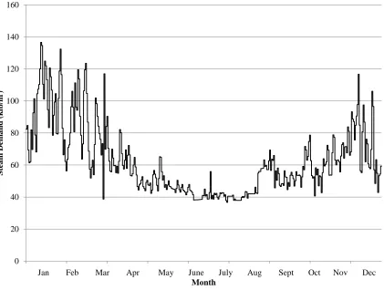
Figure 5.3. Main Campus Hourly Annual Steam Demand

This data is highly important in analyzing the overall efficiency of the cogeneration system. Steam demand in the summer is of particular importance since this value can dictate the difference between the potential amount of steam provided by the HRSG and the amount of steam that can actually be used by the campus.

5.3

Cooling

The campus utility plants also provide chilled water to the majority of campus. Chilled water 0 20 40 60 80 100 120 140 160

0 1,000 2,000 3,000 4,000 5,000 6,000 7,000 8,000

S te a m D em a n d ( k lb/ hr ) Month

water demand is serviced by 2,000 ton dual compressor chillers. These chillers allow 1,000 tons worth of chilled water to be supplied by one of the compressor units within the chiller. Once demand on that particular unit surpasses 1,000 tons, the other compressor is turned on and the load is split. This allows for more efficient part load efficiencies.

A study of the chiller system on campus revealed manufacturer performance data on efficiency. The following chart shows chiller efficiency in terms of kW/ton at a range of loading schemes as per manufacturer data.

Figure 5.4. Chiller Performance Curves from Manufacturer Data 0 0.1 0.2 0.3 0.4 0.5 0.6 0.7 0.8

0% 10% 20% 30% 40% 50% 60% 70% 80% 90% 100%

Campus chilled water demand is also important for analysis that will be conducted in this thesis. Absorption and steam turbine driven chillers will be analyzed in Chapter 8, so a clear understanding of the chilled water demand and existing chiller efficiency is needed. Daily ton-hr values data for both campus chilled water plants were obtained from documentation [20] submitted to NC State University and are shown below.

Apr May Jun July Aug Sep Oct Nov Dec Jan Feb Mar

D aily T o n -h rs

Apr May Jun July Aug Sep Oct Nov Dec Jan Feb Mar

Chapter 6

Installed System

The Raleigh campus of North Carolina State University has an aging campus steam system with a weighted average boiler age of over 45 years. Steam demand is expected to grow from the current level of approximately 200,000 pounds per hour to over 300,000 pounds per hour in the next 20 years. As such, facilities personnel and capital project managers at the University saw the need to examine possibilities for expansion and retrofit of the steam system. After initial analyses were performed, the University decided that some of the additional steam demand could be provided by waste heat fired heat recovery steam generators supplied by combustion turbines. This led to the release of a Request for Proposals (RFP) in 2009 in an effort to find a suitable contractor to perform the steam system retrofit and install the gas turbine cogeneration system.

contract generally requires the ESCO to guarantee the cost savings that will be provided by the installed system. These cost savings are then used to pay the cost of the loan financing for the project. The ESCO acts as the general contractor for the customer, securing all subcontractors and materials, as well as conducting any measurement and verification of savings (sometimes subcontracted).

Though the savings are guaranteed (to some extent) in the performance contract, when the loan is paid off, the contract ends as well as the savings guarantee. If performance is not carefully examined, then after the length of contract the customer could begin to actually lose money with no way of recovering those lost savings. This is a particularly important issue where savings are very closely tied to volatile fuel prices (ie. natural gas fired turbines).

6.1

Gas Turbines

The primary pieces of packaged equipment to be considered for the cogeneration system are the gas turbines. The choice of gas turbine affects the power produced, the fuel consumed, as well as the steam produced by any waste heat recovery steam generators. The accepted proposal chose two Solar Taurus 60-7901S 5.6 MW (ISO) combustion turbines. Included in the scope of the project are the gas turbine assemblies, two natural gas compressors, and any additional materials and installation costs associated with the turbines.

Figure 6.1. Complete Packaged Gas Turbine Assembly [19]

Control Panel Turbine Air Inlet