1
QUANTUM COMPUTING IN FOUR SPATIAL DIMENSIONS
Arturo Tozzi (Corresponding author)
Center for Nonlinear Science, University of North Texas 1155 Union Circle, #311427
Denton, TX 76203-5017 USA [email protected]
[email protected] Muhammad Zubair Ahmad
Department of Electrical and Computer Engineering University of Manitoba
Winnipeg, Canada
[email protected] James F. Peters
Department of Electrical and Computer Engineering, University of Manitoba 75A Chancellor’s Circle
Winnipeg, MB R3T 5V6 CANADA [email protected]
ABSTRACT
Relationships among near set theory, shape maps and recent accounts of the Quantum Hall effect pave the way to quantum computations performed in higher dimensions. We illustrate the operational procedure to build a quantum computer able to detect, assess and quantify a fourth spatial dimension. We show how, starting from two-dimensional shapes embedded in a 2D topological charge pump, it is feasible to achieve the corresponding four-dimensional shapes, which encompass a larger amount of information. This novel, relatively straightforward architecture not only permits to increase the amount of available qbits in a fixed volume, but also converges towards a solution to the problem of optical computers, that are not allowed to tackle quantum entanglement through their canonical superposition of electromagnetic waves.
KEYWORDS: Hall effect; oscillations; fourth dimension; computer; superlattice.
Multidimensional approaches are a novel field of research, with a potential to provide insights into physical and biological organization. However, it is currently technically demanding to cope with these elusive multidimensional activities. The recent onset of datasets encompassing thousands of features has led to the development of novel tools, such as feature selection, to model the underlying high-dimensional settings of data generation (Garcia et al., 2018). Despite feature selection techniques allow the reduction of the data dimensionality and improve algorithms’ performance (Dmochowski et al., 2017), huge data volume makes learning tasks computationally demanding. Increasing features’ quantity/complexity results in reduced computational efficiency of algorithms. Most of the algorithms in use, developed for datasets of small size, cannot cope with the emerging Big Data problems. Therefore, novel tools are required to quantify multidimensional issues related to mathematical, physical and biological systems.
2
In quantum computing, quantum properties can be used to represent and structure data (stored in terms of qbits), providing an amount of information higher than the classical computers. Here we describe a novel quantum computing tool that is able, starting from simple shapes traces encompassed in a two-dimensional lattice, to detect information from a fourth spatial dimension. We aim to transfer the framework of the quantum Hall effects provided by Lohse et al. (2018) to the realm of quantum computing, to demonstrate the feasibility of a synthetic quantum network equipped with four spatial dimensions (plus time), instead of the classical three (plus time).
We will describe 4D quantum computing in terms of a computational device able to cope with shape maps, i.e., shapes’ assessment at various hierarchical levels of synthesis. At first, we will define the fundamental structure for maps construction; then we will provide the operational steps for achieving 4D quantum computing. We will also show that shape maps provide an expanded view of the Borsuk-Ulam Theorem (Tozzi et al., 2017) which allows to increase the amount of available qbits.
INTRODUCING SHAPE MAPS
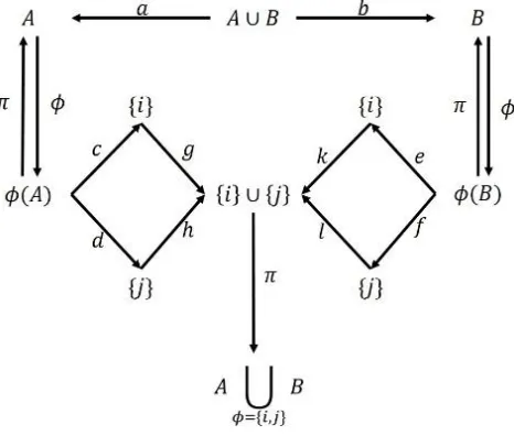
In near set theory, we consider a space 𝐾 and a probe function 𝜙: 2𝐾→ ℝ𝑛(Peters, 2007; Peters 2014). Given a a small neighborhood 𝑈 ⊂ 𝐾, we construct the fiber bundle (𝐾Φ, 𝐾, 𝜋, 𝜙(𝑈)). Here𝐾Φ is termed the glossa (a set paired with description (Ahmad, Peters, 2018)), i.e., a space where each 𝑘 ∈ 𝐾 is paired with 𝜙(𝑘), due to the local trivialization property. This structure can be described as follows:
𝜙(𝑈) → 𝐾Φ 𝜋 → 𝐾.
To define classical set theoretic operations incorporating description, we introduce the notion of descriptive intersection (Di Concilio et al., 2018). Let 𝐴, 𝐵 ⊂ 𝐾 and 𝜙: 2𝐾→ ℝ𝑛. A descriptive intersection is defined as:
𝐴 ⋂ 𝐵 = {𝑥 ∈ 𝐴 ∪ 𝐵: 𝜙(𝑥) ∈ 𝜙(𝐴) 𝑎𝑛𝑑 𝜙(𝑥) ∈ 𝜙(𝐵) }. Φ
Note that a descriptive intersection of sets 𝐴, 𝐵 consists of all the elements. in either 𝐴 or 𝐵, having the same description. It follows that all the elements in 𝐴 ∩ 𝐵 are included in the descriptive intersection. We can represent this definition in terms of fiber bundle structure and classical set theoretic operations as follows:
Once established the notion of descriptive intersection, the next step is to define a descriptive union. Four different possible definitions have been discussed byAhmad and Peters (2018): they consider either elements in 𝐴 ∪ 𝐵(non-restrictive), or 𝐴 ∩ 𝐵(restrictive), or few values of description (descriptive discriminatory), or all possible values (descriptive nondiscriminatory). Here we will evaluate just the non-restrictive and descriptive discriminatory union. Given 𝐴, 𝐵 ⊂ 𝐾 and 𝜙 ∶ 2𝐾→ ℝ𝑛, non-restrictive and descriptive discriminatory union is described as follows:
𝐴 ⋃ 𝐵 𝜙={𝑖,𝑗}
3
A non-restrictive and descriptive discriminatory union of sets A,B consists of all the elements of A and B that have matching description values {i,j}, decided a priori. A more detailed account of the properties of this union is given in Ahmad and Peters (2018). In terms of classical set theoretic operations and fiber bundles, the latter definition can be described in the following terms:
Shapes in terms of synthesis. The next step is to define representation of a shape as a synthesis. We begin with a set of shapes{𝑆ℎ𝑖}𝑖∈ℤ with no description attached to them. For simplicity, we assume them as embedded in a 2-dimensional space. This set of shapes is said to be at synthesis level 0, which is represented as𝑆0. To attach description to these shapes, we use a probe function𝜙1: 2𝑆0 → ℝ𝑛at level 0 and achieve a gloss are presented as{𝑆ℎ𝑖→ 𝜙1(𝑆ℎ𝑖)}𝑖∈ℤ, standing for the synthesis level 1 or𝑆1. We move onto the next level of synthesis, attaching another description to the one already attached in𝑆1. Thus,𝑆2 is constructed using a probe function𝜙2: 2𝑆1 → ℝ𝑛. The corresponding glossa can be represented as{𝑆ℎ𝑖→ 𝜙1(𝑆ℎ𝑖) → 𝜙2(𝜙1(𝑆ℎ𝑖))}𝑖∈ℤ. We generalize for the 𝑚𝑡ℎ synthesis level𝑆𝑚, using the probe function𝜙𝑚: 2𝑆𝑚→ ℝ𝑛. This means that the glossa at𝑆𝑚 can be written as{𝑆ℎ𝑖→ 𝜙1(𝑆ℎ𝑖) → ⋯ → 𝜙𝑚−1(⋯ 𝜙1(𝑆ℎ𝑖)) → 𝜙𝑚(𝜙𝑚−1⋯ 𝜙1(𝑆ℎ𝑖))}𝑖∈ℤ. In sum, we define a family of functions that can be collectively termed as shape maps. Let𝑠𝑖𝑖+1 : 𝑆
𝑖→ 𝑆𝑖+1, be a map between the synthesis levels, then for a shape representation with 𝑚 synthesis levels the shape maps are𝕊𝑚= {𝑠𝑖𝑖+1}𝑖=1,2,⋯,𝑚−1.
Figure 1A shows a shape map encompassing different levels of synthesis. The shapes 𝑆ℎ𝑖, exist at 𝑆0the zeroth level of synthesis. At 𝑆1, descriptions are attached to each shape with the help of a probe function 𝜙1. At the next level of synthesis, a description is attached to the description of each of the objects by 𝜙2. Similarly, increasing the levels of synthesis, we increase the number of descriptions until, at 𝑆𝑛, a description is attached to the previous level using𝜙𝑛. At the highest level, the description can be written as a composition of maps 𝜙𝑛(𝜙𝑛−1⋯ 𝜙1(𝑆ℎ𝑖)).
Once achieved shapes representation with the desired level of synthesis, we need to “organize” them according to a general description throughout all the levels. By “organizing” we mean clustering the shapes into sets based on some similarity criterion. Here the previously described near set paradigm comes into play. For this purpose, the descriptive intersection (Di Concilio et al., 2018) and the non-restrictive and descriptive discriminatory union
4 𝒪𝑗= {⋂
Φ
, { ⋃ 𝜙=𝐴𝑖∈𝐴
}
𝑖∈ℤ
} , 𝑤ℎ𝑒𝑟𝑒 𝐴 = {𝑥 ∈ 2𝑪𝒐𝒅𝒐𝒎𝒂𝒊𝒏(𝝓𝒋): |𝑥| = 2}.
In this set, we achieve both descriptive intersection and a selection of the possible non-restrictive and descriptive discriminatory unions. Further, if we take into account any of these operators for𝑆𝑖, the synthesis assesses the descriptions attached at𝑆𝑖and provides again the elements of the 𝑆𝑖−1 level. This is clear from the arrow diagrams illustrated in Figure 1A, which show how the descriptive set theoretic operations return the elements in the base space 𝐾, rather than the ones in the glossa 𝐾Φ. We assume that each of the operators in𝒪𝑗 can be used for a single set, instead of canonical binary operator. The same applies for the descriptive union in which all the elements with a priori decided descriptions are returned. We define a family of maps, which clusters the elements in𝑆𝑖 based on the application of operators in𝒪𝑖:
𝒞𝑖= {𝑐𝑗𝑖= 𝑠𝑖−1𝑖 (𝒪𝑗𝑖(𝑆𝑖−1))}𝑗=1,2,⋯,|𝒪𝑖|where, 𝒪𝑗𝑖 is the𝑗𝑡ℎ element of the set𝒪𝑖.
This map clusters the elements in𝑆𝑖 based on some similarity measure. If we consider the non-restrictive and descriptive discriminatory union with 𝜙 = {𝑖, 𝑗} as the similarity measure, then it results in clustering all the shapes with description value of either 𝑖 or 𝑗. Every operator in𝒪𝑖 results in a different cluster (set) of 𝑆𝑖elements. Because each𝑐𝑗𝑖: 𝑆𝑖−1 → 𝑆𝑖, their union to form𝒞𝑖 results in a new space 𝑃(𝑆𝑖), built by clustering the𝑆𝑖elements. Hence, we can represent this as𝒞𝑖: 𝑆𝑖−1 → 𝑃(𝑆𝑖). An example of this map is illustrated in Figure 1B. This Figure also illustrates the beginning of a hyper Borsuk-Ulam Theorem (Borsuk, 1957-58; Matoušek 2003; Tozzi and Peters 2016a). The introduction of a hyper-BUT paves the way to techniques for shape detection, “bunching” (clustering), classification, building (disparate shapes are synthesized to form new shapes for future reference), and shape analysis in a high-dimensional space (Tozzi and Peters 2016). Shape building, also called bulk building, allows new shapes to be achieved. The hierarchical view of shape maps leads to two forms of synthesis, namely, shape-gluing (descriptive intersection) and shape agglomeration (descriptive union).We define another family of maps for synthesis level 𝑚 represented asℭ𝑚= {𝐶𝑖}𝑖=1,2,⋯𝑚, termed clustering maps. This allows to build a diagram termed
5
6 A TOOL FROM THEORETICAL PHYSICS
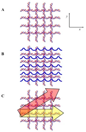
Here we ask: is it feasible to assess and quantify how quantum oscillations may generate multidimensional computations? More specifically, is it feasible to build a real or an artificial oscillatory network able to simulate an otherwise undetectable fourth spatial dimension? The answer is affirmative. Recent experimental findings describe a technique that throws an operational bridge between theoretical physics and quantum computing. At first, we explore the “Hall effect” (Hall, 1879), i.e., the production of potential difference transverse to electric current, upon application of a magnetic field perpendicular to current. Magnetic fields with the proper angulation are able to bend electric rays. A comparable phenomenon, called “quantum Hall effect”, occurs in quantum dynamics (Novoselov et al., 2007). An electric charge sandwiched between two surfaces behaves like a two-dimensional material: when this material is cooled down to near absolute-zero temperature and subjected to a strong magnetic field, the amount that it can conduct becomes “quantized”, leading to the so-called quantum Hall effect (Tozzi, 2019). This puzzling phenomenon is easily explained, if we take into account that it occurs in four, instead of the canonical three, spatial dimensions (Zhang and Hu 2001; Kraus et al., 2013; Zilberberg et al., 2018). Lohse et al. (2018) found a (relatively) simple way to probe four-dimensional quantum physical phenomena, starting from an artificial, two-dimensional dynamic system, a superlattice termed“2D topological charge pump”. The light flowing through the two-dimensional superlattice behaves according to the predictions of the four-two-dimensional quantum Hall effect. The Authors provided a two-dimensional waveguide equipped with patterns acting as manifestations of higher-dimensional coordinates: in operational terms, they built a 2D lattice consisting of superlattices along the x and y axes. Each superlattice is achieved by superimposing two standing waves of different wavelength (Figure 2A). When a third wave is introduced along the x direction, this corresponds to tilting the long lattice along a one-dimensional path shadowing the axis x, carefully choosing the proper inclination (Figure 2B). Lohse et al. (2018) and Zilberberg et al. (2018) provided the proper measures (e.g., angles, equations) to detect the 4D quantum Hall effect. Their procedure on 2D topological charge pumps allows the achievement of dynamics along the y axis that are equivalent to movements in four spatial dimensions. They attained two different responses: a linear one (two-dimensional response) along the axis x and a nonlinear one (four-(two-dimensional response) along they axis (Figure 2C). In sum, the Authors provide a technique which describes quantum dynamics in terms of pure oscillations. Here we ask: could such procedure be transferred, with the due corrections, to quantum computing, in order to build a spatial four-dimensional device where quantum computational operations might take place?
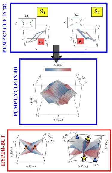
Computations in the form of shape maps. In the previous paragraph, we showed that Lohse et al.’s (2018) approach, i.e., a 2D topological charge pump, holds true for the assessment of the unusual multidimensional phenomenon occurring in quantum dynamics’ Hall effect. Here we aim to show how, with the proper amendments, their four-dimensional- apparatus could be also used to build, assess and quantify a further spatial dimension of quantum computers endowed in two-dimensional lattices. In other terms, our aim is to explore 4D shapes using 2D functional lattices, where the constructing basis in the x and the y dimensions are superlattices, i.e., periodic layered structures derived from the superposition of two stationary waves of different wavelengths. Our goal is to correlate shape maps to Lohse’ et al.’s 2D lattice oscillations, the latter standing for the S0 at the Oth level of synthesis (Figure 3, lowest part). The entire topological pump stands for the space K, while its horizontal and vertical oscillations stand, respectively, for 𝐴, 𝐵 ⊂ 𝐾. The topological pump’s phase φx(which is the pump parameter, achieved when pumping is performed by moving the long lattice along x) stands for the probe function φ1 displayed in Figure 1A. The topological pump’s phase φy(which stands for a transverse superlattice phase that depends linearly on x, and which varies with φx changes) stands for the probe function φ2. Note that φx lies at the S1 level of synthesis, while φy at the S2 level. In sum, when φx is modified, we achieve changes in φy, which lead to a quantized non-linear response along y: such nonlinear response stands for the four-dimensional features in the topological space K. Note that, when an adiabatic pump cycle of the 2D topological charge pump is performed (Figure 4), we achieve periodic modulation along closed trajectories, both on the horizontal and vertical plane (curves φx and φx in the upper part of the Figure 4). In a full pump cycle, these closed trajectories cover a closed surface which lies in the 4D parameter space (middle part of Figure 4).
7
multidimensional structure equipped with antipodal features with matching description, in touch with Peters and Tozzi (2016), who suggested quantum entanglement as occurring in four spatial dimensions.
8
9
10
correspond to planes that touch at the origin, it is easy to detect several antipodal points with matching description (green and blue triangles, yellow stars). See Lohse et al. (2018) for further details and the legenda of the plots depicted here.
CONCLUSIONS
We aimed to transfer the framework of the quantum Hall effect provided by Lohse et al. (2018) to the realm of quantum computation, in order to: a) describe real multidimensional mathematical/physical/biological dynamics and b) demonstrate the feasibility of a synthetic network equipped with four spatial dimensions (plus time), instead of the classical three (plus time). We provide the theoretical apparatus to link 2D topological charge pump to topological shape maps, achieving quantum computing in four spatial dimensions. Indeed, working on a properly manipulated two-dimensional quantum lattice such as the 2D topological charge pump, it is feasible to build a transverse oscillation standing for the whole system’s four-dimensional component. We showed how the superimposition of waves of different frequency and orientation produces the required superlattice’s functional reticulum. When the latter is crossed by other waves of different frequency along its x axis, both (two-dimensional) linear and (four-dimensional) nonlinear dynamics are accomplished. The superimposition of the proper waves gives rise to two quantifiable and assessable different motions: a linear one along the x axis, and a nonlinear one along the y axis. The oscillatory response along the y axis stands for the artificial network’s component displaying the fourth spatial dimension.
The question is: why might scientist perform computations in four spatial dimensions, instead of the canonical three? How much could quantum computing profit from operations taking place in higher dimensions? When projecting qbits from lower to higher dimensions, their number increases, due to the dictates of the recently-developed variants of the Borsuk-Ulam theorem (Tozzi and Peters, 2016b). Taking into account our framework, the shape projection from two to four spatial dimensions allows to achieve FOUR shapes with matching description, because the mappings takes place two dimensions higher. This means that a 4D quantum computer (built on an easily manageable 2D lattice) amplifies four times the same message (which can be described in terms of qbits), but does not require increases in phase space’s volume: indeed, going in higher dimensions, the manifold volume does not increase, while the information does. In other words, the interaction among different waves produces a novel functional dimension, i.e., a higher dimensional phase space where computational operations take place more efficiently at the same energetic cost.
To provide a theoretical operational example, in a visual 2D scene the presence of the shape causes a deformation in 2D topological charge pumps. The resulting 4D wave stands for the computer’s response to the introduction of the object in its oscillatory lattice. Therefore, 4D oscillation is the main feature that multiplies the number of shapes. Further, the x and y axes can be arranged in varying orientations according to different required shape reconstructions, allowing to increase discriminatory power and detectable features. Also, the fourth dimension overtakes one of the current limitations of optical quantum computing, i.e, the impossibility to achieve quantum entanglement. Indeed, entangles particles, hidden in lower dimensions, are detectable in higher ones, as demonstrated by Peters and Tozzi (2016). The last, but not the least, different mathematical/physical/biological activities might exhibit different four-dimensional hidden components, that, once detected, could be experimentally assessed and quantified.
REFERENCES
1) Ahmad MZ, Peters JF. 2018. Descriptive unions. A fibre bundle characterization of the union of descriptively near sets, arXiv 1811, no. 11129, 1-19.
2) Borsuk K. 1957-58. Concerning the classification of topological spaces from the standpoint of the theory of retracts, XLVI, 177–190.
3) Di Concilio A, Guadagni C, Peters JF, RamannaS. 2018. Descriptive proximities. Properties and interplay between classical proximities and overlap. Mathematics in Computer Science 12, no. 1, 91-106. 4) Dmochowski JP, Ki JJ, DeGuzman P, Sajda P, Parra LC. 2017. Extracting multidimensional
11
5) Garcia JO, Ashourvan A, Muldoon SF, Vettel J, Bassett DS. 2018. Applications of Community Detection Techniques to Brain Graphs: Algorithmic Considerations and Implications for Neural Function. Proceedings of the IEEE PP(99):1-22. DOI10.1109/JPROC.2017.2786710.
6) Hall E. 1879. On a New Action of the Magnet on Electric Currents. American Journal of Mathematics. 2 (3): 287–92. doi:10.2307/2369245.
7) Kraus YE, Ringel Z, Zilberberg, O. 2013. Four-dimensional quantum Hall effect in a two-dimensional quasicrystal. Phys. Rev. Lett. 111, 226401.
8) Lohse M, Schweizer C, Price HM, Zilberberg O, Bloch I. 2018. Exploring 4D quantum Hall physics with a 2D topological charge pump. Nature 553, 55–58. doi:10.1038/nature25000.
9) Matoušek J. 2003. Using the Borsuk–Ulam Theorem. Lectures on Topological Methods in Combinatorics and Geometry. Springer-Verlag Berlin Heidelberg, 2003
10) Novoselov KS, Jiang Z, Zhang Y, Morozov SV; Stormer HL, et al. 2007). Room-temperature quantum Hall effect in graphene. Science. 315 (5817): 1379.
11) Peters JF. 2007. Near sets. Special theory about nearness of objects. FundamentaInformaticae 75, nos. 1-4, 407-433.
12) Peters JF. 2014. Topology of Digital Images. Visual Pattern Discovery in Proximity Spaces, Intelligent Systems Reference Library, vol. 63, Springer, ISBN 978-3-642-53844-5, pp. 1-342.
13) Peters JF, Tozzi A. 2016. Quantum Entanglement on a Hypersphere. Int J Theoret Phys, 1–8. doi:10.1007/s10773-016-2998-7.
14) Tozzi A, Peters JF. 2016a. Towards a Fourth Spatial Dimension of Brain Activity. Cognitive Neurodynamics 10 (3): 189–199. doi:10.1007/s11571-016-9379-z.
15) Tozzi A, Peters JF. 2016b. A Topological Approach Unveils System Invariances and Broken Symmetries in the Brain. Journal of Neuroscience Research 94 (5): 351–65. doi:10.1002/jnr.23720.
16) Tozzi A, Peters JF, Fingelkurts AA, Fingelkurts AA, Marijuán PC. 2017. Topodynamics of metastable brains. Physics of Life Reviews, 21, 1-20. http://dx.doi.org/10.1016/j.plrev.2017.03.001.
17) Tozzi A. 2019. The multidimensional brain. Physics of Life Reviews. doi: https://doi.org/10.1016/j.plrev.2018.12.004. In press.
18) Zhang, S-C, Hu J. 2001. A four-dimensional generalization of the quantum Hall effect. Science 294, 823– 828.