Method of Generating Contexts based on
Self-adaptive Differential Particle Swarm using Local
Topology for Multimodal Optimization in the case of
Multigranulation. A Case Study
Dianne Arias1 0000-0002-4715-5419, Yaima Filiberto1* 0000-0003-2279-2953 and Rafael Bello 2, 0000-0001-5567-2638
1 University of Camaguey 1; [email protected], [email protected] 2 University of Las Villas 2; [email protected]
* Correspondence: [email protected]; Tel.: +5353559573
Version January 11, 2019 submitted to Preprints
Abstract:Multigranulation is a new approach to the Rough Set Theory, where several separability 1
relationships are used to obtain different granulations of the universe. The Multigranulation starts 2
from the existence of different contexts or subsets of features to characterize the objects of the universe. 3
In this paper, a method for the generation of contexts from the construction of similarity relations is 4
proposed.The proposed solution was evaluated in an international database using the KNN classifier. 5
It was also applied in the solution of a real problem in Civil Engineering specifically in Traffic 6
Engineering, the contexts generated from the proposal used to determine the features of higher 7
incidence in the service level of the road. The results achieved both in the international database and 8
in the proposed application demonstrate the applicability of the proposed method. 9
Keywords:multigranulation; separability relationships; service level of the road 10
0. Introduction 11
Rough set theory, originated by Pawlak [1][2][3], has become a well-established mechanism for 12
uncertainty management in a wide variety of applications related to artificial intelligence [4][5][6][7]. 13
One of the strengths of rough set theory is that all its parameters are obtained from the given data. 14
This can be seen in the following paragraph from [8]: 15
"The numerical value of imprecision is not pre-assumed, as it is in probability theory or fuzzy sets 16
but is calculated on the basis of approximations which are the fundamental concepts used to express 17
imprecision of knowledge". In other words, instead of using, the rough set data analysis (RSDA) 18
utilizes solely the granularity structure of the given data, expressed as classes of suitable equivalence 19
relations. 20
In the past 10 years, several extensions of the rough set model have been proposed in terms of various 21
requirements, such as the variable precision rough set (VPRS) model [9], the rough set model based on 22
tolerance relation [10], the Bayesian rough set model [11], the fuzzy rough set model and the rough 23
fuzzy set model [12]. 24
In many circumstances, we often need to describe concurrently a target concept through multi binary 25
relations according to a users requirements or targets of problem solving, for that another extension of 26
the RST is to use more than one separability relationship to perform the granulation of the universe, 27
which is known as multigranulation [13][14]. In this case, from the set of predictive features A, two 28
or more subsets A1, ...,Ak, Ai Am ⊆ A, are formed of features that allow defining the separability 29
relation. These subsets of features are called contexts [15]. Based on this multigranulation approach, 30
different techniques for the discovery of knowledge have been formulated. 31
1. Multigranulation in the Rough Set Theory 32
Qian et al. [13] proposed multigranulation rough set (MGRS) in complete information system to 33
more widely apply rough set theory in practical applications, in which lower/upper approximations 34
are approximated by granular structures induced by multi binary relations. The multigranulation 35
rough set is different from Pawlaks rough set model because the latter is constructed on the basis 36
of a family of indiscernibility relations instead of single indiscernibility relation. In optimistic 37
multigranulation rough set approach, the word "optimistic" is used to express the idea that in multi 38
independent granular structures, we need only at least one granular structure to satisfy with the 39
inclusion condition between equivalence class and the approximated target. The upper approximation 40
of optimistic multigranulation rough set is defined by the complement of the lower approximation[37]. 41
From the point of view of the applications of the RST, the multigranulation in the RST is very 42
desirable in many real applications, such as analysis of data from multiple sources, discovery of 43
knowledge to from data with large dimensions and distributive information systems. Since Qian in 44
2006 proposed multigranulation in the RST, the theoretical framework has been widely enriched, and 45
many extensions of these models have been proposed and studied[35][36]. In the mutigranulation 46
rough set theory, each of various binary relation determines a corresponding information granulation, 47
which largely impacts the commonality between each of the granulations and the fusion among all 48
granulations. 49
In their papers, Qian et al. said that the MGRS are useful in the following cases: 50
51
1. We cannot perform the intersection operations between their quotient sets and the target concept 52
cannot be approximated by usingU/(PS
Q)which is called a single granulation in those papers. 53
54
2. In the process of some decision making, the decision or the view of each of decision makers 55
may be independent for the same project (or a sample, object and element) in the universe. In 56
this situation, the intersection operations between any two quotient sets will be redundant for 57
decision making. 58
59
3. Extract decision rules from distributive information systems and groups of intelligent agents 60
through using rough setapproaches. 61
62
Since then,many researchers have extended the classical MGRS by using various generalized binary 63
relations. 64
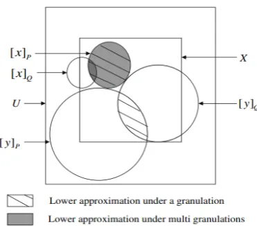
In Fig.1 of the author Qian in [13], the bias region is the lower approximation of a setXobtained by a 65
single granulation PS
Q, which is expressed by the equivalence classes in the quotient set U/(PS
Q), 66
and the shaded region is the lower approximation ofXinduced by two granulations P+Q, which is 67
Figure 1.Difference between Pawlaks rough set model and MGRS.
From the point of view of the applications of the RST, the multigranulation in the RST is very 69
desirable in many real applications, such as analysis of data from multiple sources, discovery of 70
knowledge to from data with large dimensions and distributive information systems. 71
72
2. Self-Adaptive Differential Particle Swarm using a local topology for Multimodal Optimization 73
Particle Swarm Optimization is an effective and robust non-direct global-search method for 74
solving challenging continuous optimization problems. The PSO meta-heuristic involves a set of 75
particles known as swarm which explore the search space trying to locate promising regions [32]. 76
Therefore, particles are interpreted as solutions for the optimization problem and they are represented 77
as points inn-dimensional search space. In the case of standard PSO, each particleXimoves through 78
the space using its own velocityVi, a local memory of the best position it has obtainedPiand knowledge 79
of the best solutionGfound in its neighborhood. Equations1and2show how to update the particles 80
position based on the mentioned components. 81
ϑi(t+1) = α∗ϑi(t) +U(0,ϕ1)(pBest(t)−xi)
+U(0,ϕ2(gBest(t)−xi) (1)
xi(t+1) =xi(t)ϑi(t+1) (2) In last decades Evolutionary and Swarm Intelligence algorithms have become an important improvement for both discrete and real-parameter optimization. Without niching [34] strategies they converge to a single optimum, even in multimodal search spaces where numerous global or local solutions exist. However, most real-life problems are characterized by multimodal functions. In literature several niching approaches have been proposed for computing multiple optima simultaneously, though most of them require some user-specified parameters that should be estimated in advanced (i.e. additional knowledge about problem domain is required)[34].
Then, multimodal optimization methods try to discover and maintain multiple subpopulations in a single run, where each niche corresponds to a specific peak of the fitness landscape (ideally one species per optimum). They have been developed to reduce the undesirable effects of genetic drift. In few words, niching strategies should be able to preserve the diversity in the artificial population, allowing individuals parallel convergence toward different solutions. As well, niching methods are useful to avoid stagnation or premature convergence states in global optimization problems where many sub-optimal solutions exist; offering an escaping alternative from local optima [34].
optima. Ironically, it is the slightly interaction among particles that is most responsible of the poor performance of the PSO based algorithms using a Ring Topology. To improve the search capability of such models a novel Differential Operator is introduced. This operator is straightforwardly inspired on the well-known differential strategy DE/current-to-rand/1 without crossover [33]. Therefore, as first step, we design a mutation operator as illustrate following equation3.
e
xi(t+1) =pBesti(t) +F∗(pBestr1(t)−pBestr2(t)) (3)
WherepBesti(t)denotes the personal best position of current individual,pBestr1(t)andpBestr2(t)are
the global best record achieved by two randomly selected swarm particles.
Next, a selection operation takes place, wherexeiis accepted as current particle position if it improves the search procedures, respect to the solution generated by the PSO rules; otherwise the mutant is rejected (See in equation4)[34].
xti+1=
xti+1,si fxei t+1
≤ fPit+1 xti+1,si fxei
t+1
> fPit+1 (4)
Following a similar reasoning of the conventional clearing, it’s used a novel diversity procedure: Heuristic Clearing. It is able to preserve the swarm diversity in lbest PSO algorithms using a Ring Topology based topology, and it does not need to be specified any niche parameter. To do that, this operator only takes into account optimal particles (See equation5)[34].
| f(Pi)−F∗|<ε (5)
In the following section we propose a method to generate contexts using multigranulation based on 82
the rough set theory and multimodal PSO. 83
3. Method of Generating Contexts based on Self-adaptive Differential Particle Swarm using 84
Local Topology for Multimodal Optimization in the case of Multigranulation. 85
Be a decision systemSD=AS
dwhere the domain of the characteristic inAS
dmay be discrete 86
or continuous values, from which calculate the features weights using the PSOMulti+RST+MG method, 87
which is a modification of PSO + RST [17]. In this case PSO Multimodal is used in order to obtain 88
multiple maximums global (gbest) from which the set of contexts is created and the number of 89
characteristics per context, then weights are ordered by contexts and those with a weight greater than 90
the mean value are selected of the weight for that context. Finally the same contexts are remove. The 91
algorithm is described below. 92
Algorithm 1Pseudocode for PSOMulti+RST+MG algorithm
1. Calculate the weights (w) of features using PSOMulti+RST method. 2. Generate set of contexts using GBest(Φn)
C=Φn
3. For each contextCi: OrderWi
SelectWij∈Wimax⇐⇒ {Wij>mean(Wi)} 4. Select de different context
∀Ci,Cj|Ci,Cj∃C∧Ci6=Cj
Algorithm PSOMULTI+RST+MG
Step 2:For each particle, evaluate the quality measure of similarity using expression6, inDVariables.
max→
∑
∀xeU ϕ(x) |U|
(6)
Step 3: Compare the quality measure of the current similarity of each particle with the quality 93
measurement of the similarity of your previous best position pBest. If the current value is better 94
than that ofpBest, then assign topBestthe current value, andpBest=xi, that is, the current location 95
becomes the best one so far. 96
Step 4:Identify the particle in the neighborhood with the highest value for the quality of similarity 97
measure and assign its index to the variablegBestand assign the best value of the quality measure of 98
similarity tom. 99
Step 5: Adjust the speed and position of the particle according to equations1,2and3(for each 100
dimension). 101
Step 6:Verify if the stop criterion is met (maximum number of iterations or if it takes five iterations 102
without improving the quality measure of the global similarity (m)), if not, go to Step2. 103
104
4. Experimental results 105
For this study we used data sets from the UCI repository [38] (iris, schizo, hepatitis,biomed, 106
glass,analcaabankruptcy,diabetes,liver−disorders,ecoli,vehicle,lungcancer,segment,new−thyroid, 107
breast−w,bupa). It is used to calculate the weights forKNN[23] withk= 1 the proposed method. 108
The training and test sets were obtained, taking 75 percent of the cases for the first and 25 percent for 109
the second, in a totally randomized manner. Following this principle of random selection the process 110
was repeated ten times and ten training sets and ten test sets were obtained for each data set, in order 111
to apply cross validation [24] for a better validation of the results. 112
The parameters used in the experimentation, for the methodPSOMulti+RST+MGwere:TB= 40, 113
N I= 100,ce1 =ce2 = 2 and the values ofe1 ande2 for the function of similarity between attributes 114
and for the function of similarity for the decision attribute were between 0.70-0.83 and 1.0,F=0.1. The 115
stop condition is: when 100 iterations are reached or when in five iterations the fitness value does not 116
improve (measure quality similarity quality). 117
It is used as aKNNclassifier withK= 1 to make a comparison of the results obtained after the creation 118
of the proposed method’s contexts PSOMULT I+RST+MG with algorithms AdaBoostM1[30], 119
RandomSubSpace[31] andBagging [29], implemented in the WEKA1 tool and using theKNN as 120
a classifier, in all cases. 121
For the statistical analysis of the results, the hypothesis testing techniques were used [25]. For multiple 122
comparisons, the Friedman and Iman-Davenport tests [26] are used to detect statistically significant 123
differences between a groups of results. The Holm test [27] is also used in order to find significantly 124
higher algorithms. 125
These tests are suggested in the studies presented in [24], which states that the use of these tests is 126
highly recommended for the validation of results in the field of automated learning. In the statistical 127
processing of all the experimental results, the KEEL was used [28]. 128
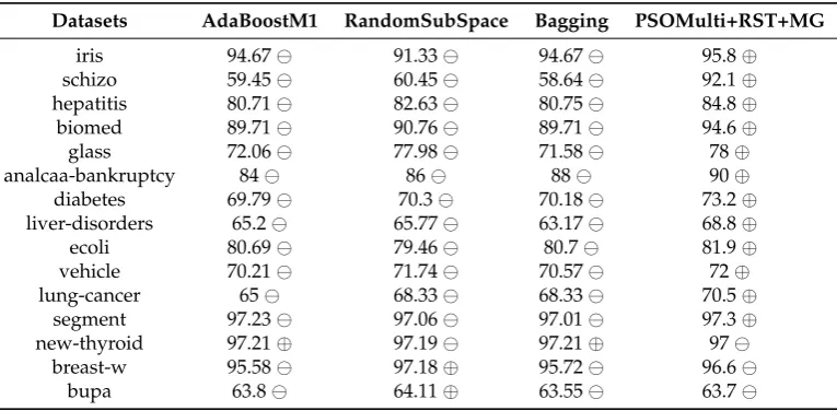
Table 1 shows the description of the data sets used in the experimentation, as well as the contexts 129
obtained by the proposed method (column 4) and the number of average features for each context 130
(column 5). Table 2 shows the results of evaluating the contexts with theKNNmethod forK= 1 (Knn 131
1 Herramienta de código abierto escrita en Java. Disponible bajo licencia pública GNU en
algorithmPSOMULT I+RST+MG), as well as the results of theAdaBoostM1,RandomSubSpaceand 132
Baggingalgorithms, as you can observe the proposed method obtains better results than the rest. 133
Table 1.Datasets
Datasets Instances Feature Contexts Features average X Contexts
iris 15 4 3 2
schizo 11 14 31 3
hepatitis 16 19 13 4
biomed 20 8 24 5
glass 22 9 34 5
analcaa-bankruptcy 5 6 10 4
diabetes 77 8 32 5
liver-disorders 35 6 19 4
ecoli 34 7 23 4
vehicle 85 18 37 5
lung-cancer 4 56 4 2
segment 231 19 13 4
new-thyroid 22 5 3 3
breast-w 70 9 30 5
bupa 35 6 13 4
Table 2.Experimental results forKNNwithK=1
Datasets AdaBoostM1 RandomSubSpace Bagging PSOMulti+RST+MG
iris 94.67 91.33 94.67 95.8⊕
schizo 59.45 60.45 58.64 92.1⊕
hepatitis 80.71 82.63 80.75 84.8⊕
biomed 89.71 90.76 89.71 94.6⊕
glass 72.06 77.98 71.58 78⊕
analcaa-bankruptcy 84 86 88 90⊕
diabetes 69.79 70.3 70.18 73.2⊕
liver-disorders 65.2 65.77 63.17 68.8⊕
ecoli 80.69 79.46 80.7 81.9⊕
vehicle 70.21 71.74 70.57 72⊕
lung-cancer 65 68.33 68.33 70.5⊕
segment 97.23 97.06 97.01 97.3⊕
new-thyroid 97.21⊕ 97.19 97.21⊕ 97
breast-w 95.58 97.18⊕ 95.72 96.6
bupa 63.8 64.11⊕ 63.55 63.7
Thus,⊕indicates that the accuracy is significantly better whenPSOMULT I+RST+MGmethod 134
is used, signifies that the accuracy is significantly worse andsignifies that there is no significant 135
differences. 136
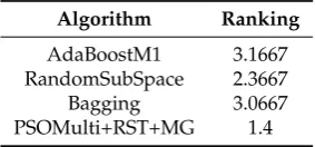
The Holm test was applied, with respect to the general accuracy of theKNN, and it is corroborated 137
that the results are significantly higher when the contexts obtained by thePSOMULT I+RST+MG 138
method are used. Tables 3 and 4 show the results of the statistical tests related to this result. 139
P-values obtained in by applying post hoc methods over the results of Friedman procedure. Average 140
Table 3.Average Rankings of the algorithms (Friedman)
Algorithm Ranking
AdaBoostM1 3.1667 RandomSubSpace 2.3667 Bagging 3.0667 PSOMulti+RST+MG 1.4
Friedman statistic (distributed according to chi-square with 3 degrees of freedom): 17.94. 142
P-value computed by Friedman Test: 0.000453. 143
144
Iman and Davenport statistic (distributed according to F-distribution with 3 and 42 degrees of 145
freedom): 9.281596. 146
P-value computed by Iman and Daveport Test: 0.000078909633. 147
148
Table 4.Post Hoc comparison Table forα=0.05 (FRIEDMAN)
i algorithm z= (R0−Ri)/SE p Holm
3 AdaBoostM1 3.747666 0.000178 0.016667
2 Bagging 3.535534 0.000407 0.025
1 RandomSubSpace 2.05061 0.040305 0.05
5. Applications of the Method in the Solution of a Real Problem 149
In this section a real problem related with the branch of the Civil Engineering is solved, using the 150
following procedure: 151
Step 1:Build the decision system for the application domain 152
Step 2:Calculate the weight using the quality of similarity measure (using PSOMulti+RST+MG) 153
Step 3:Generate set of contexts using the weight calculated inStep 2 154
Step 4:Apply the weights per contexts in the classification with KNN. 155
The concept of "Level of Service" it was presented as a means to quantify or to classify the 156
operational quality of the service offered by a road to drivers and users. It defined "Level of Service" 157
like a qualitative measure that describes the operational conditions inside the current of the traffic and 158
their perception for the driver and the passenger. A definition of level of service generally describes 159
these conditions in such terms as speed and time of journey, maneuver freedom, interruptions of the 160
traffic, comfort, comfort and security [39]. 161
162
In the level of service it influences the intensity of the vehicular interaction, the conditions of 163
the road and their environment, and the quality of the regulation and signaling of the road. They 164
have been defined six levels of service for each type of road; assigning them of the letter "A" to the "F", 165
being the level of service "A" the one that represents the best operation conditions and the level of 166
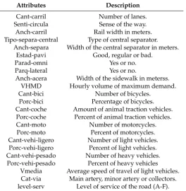
service "F", the worst conditions [39]. The problem is to predict the Level of Service. The description of 167
the dataset is shown in Table 5. 168
Table 5.Description of the data-set used in the experiment.
Attributes Description
Cant-carril Number of lanes. Senti-circula Sense of the way. Anch-carril Rail width in meters. Tipo-separa-central Type of central separator.
Anch-separa Width of the central separator in meters. Estad-pavi Good, regular or bad.
Parad-omni Yes or no.
Parq-lateral Yes or no.
Anch-acera Width of the sidewalk in meterss. VHMD Hourly volume of maximum demand. Cant-bici Number of bicycles.
Porc-bici Percentage of bicycles. Cant-coche Amount of animal traction vehicles. Porc-coche Percent of animal traction vehicles. Cant-moto Number of motorcycles. Porc-moto Percent of motorcycles. Cant-vehi-ligero Number of light vehicles. Porc-vehi-ligero Percent of light vehicles. Cant-vehi-pesado Number of heavy vehicles. Porc-vehi-pesado Percent of heavy vehicles
Vmedia Average speed of travel of light vehicles. Cat-via Main artery, minor artery or collectors. level-serv Level of service of the road (A-F).
The data used for the study were been of counts carried out in different schedules in urban roads 170
in Cuba, in the main arteries of the city of Camaguey. 171
To predict service levels of a road allows the engineers to base the decisions that propose in this 172
respect of necessities of new roads, their physical and geometric characteristics assisting at the wanted 173
levels of service. They also allow to fix corrections in existent roads, impacting on the organization of 174
the traffic or envelope the characteristics of the road with the objective of elevating the quality of the 175
operational level. The parameters used in the experimentation, for the methodPSOMulti+RST+MG 176
were: TB= 40,N I= 100,ce1 =ce2 = 2 and the values ofe1 ande2 for the function of similarity between 177
attributes and for the function of similarity for the decision attribute were 0.75 and 1.0,F=0.1. The 178
stop condition is: when 100 iterations are reached or when in five iterations the fitness value does 179
not improve (measure quality similarity quality). An experimental study for the data-set traffic is 180
performed (Table 7). 181
Table 6.Results of the general classification accuracy for level of service with 1NN.
Dataset AdaBoostM1 RandomSubSpace Bagging PSOMulti+RST+MG
Transito3 60 57.5 57.5 63.2
6. Conclusions 182
In this paper a new method of generating contexts based on similarity relationships for 183
multigranulation using Self-adaptive Differential Particle Swarm using Local Topology for Multimodal 184
Optimization is proposed. The main contribution is the construction of similarity relations based 185
on the quality of similarity measure of Rough Sets Theory as a function of membership to build 186
contexts for multigranulation. This measure calculates the degree of similarity in a decision system 187
in which the feature may have discrete or continuous values. The contexts obtained were evaluated 188
in international databases with the k-NN. The results achieved were significantly superior to the 189
compared methods, which shows the effectiveness of the proposed method. The effectiveness of the 190
related to the branches of Civil Engineering (problem of prediction of the level of service in urban 192
roads). 193
References 194
1. Pawlak,Z. Rough Sets.International Journal of Computer and Information Sciences1982,11, 341-356. 195
2. Komorowski, J. and Pawlak, Z. and Polkowski, L. and Skowron, A. Rough sets: A tutorial. Rough fuzzy 196
hybridization: A new trend in decision-making1999,11, 3-98.
197
3. Greco, S. and Matarazzo, B. and Slowinski, R. Rough sets theory for multicriteria decision analysis.European 198
journal of operational research2001,129, 1-47.
199
4. Duntsch,I., Gediga,G. Uncertainty measures of rough set prediction.Artificial Intelligence1998,106, 109-137. 200
5. Jensen,R., Shen,Q. Fuzzy-rough sets assisted attribute selection.IEEE Transactions on Fuzzy Systems2007,15, 201
73-89. 202
6. Jeon,G., Kim,D. Jeong,J. Rough sets attributes reduction based expert system in interlaced video sequences. 203
IEEE Transactions on Consumer Electronics2006,52, 1348-1355.
204
7. Liang,J.Y., Dang,C.Y., Chin,K.S., Yam Richard,C.M. A new method for measuring uncertainty and fuzziness 205
in rough set theory.International Journal of General Systems2002,31, 331-342. 206
8. Pawlak,Z. Rough Sets: Theoretical Aspects of Reasoning about Data.System Theory, Knowledge Engineering 207
and Problem Solving1991,9.
208
9. Ziarko,W. Variable precision rough sets model.Journal of Computer System Science1993,46, 39-59. 209
10. Skowron,A., Stepaniuk,J. Tolerance approximation spaces.Fundamenta Informaticae1996,27, 245-253. 210
11. Slezak,D., Ziarko,W. The investigation of the Bayesian rough set model.International Journal of Approximate 211
Reasoning2005,40, 81-91.
212
12. Dubois,D., Prade,H. Rough fuzzy sets and fuzzy rough sets.International Journal of General Systems1990,17, 213
191-209. 214
13. Qian,Y.H., Liang,J.Y., Yao,Y.Y., Dang,C.Y. MGRS: a multi-granulation rough set.Information Sciences2010, 215
180, 949-970. 216
14. Lin,G., Liang,J., Qian,Y. Multigranulation rough sets: From partition to covering.Information Sciences2013, 217
241, 101-118. 218
15. Intan,R., Mukaidono,M. Multi-rough Sets Based on Multi-contexts of Attributes.Lectures Notes on Artificial 219
Intelligence2003,2639, 279-282.
220
16. Filiberto,Y., Bello,R., Caballero,Y., Larrua,R. A method to build similarity relations into extended Rough Set 221
Theory.10th International Conference on Intelligent Systems and Applications2010,10384, 978-1-4244-8135-4. 222
17. Filiberto,Y., Bello,R., Caballero,Y., Larrua,R. Using PSO and RST to predict the resistant capacity of 223
connections in composite structures.Studies in Computational Intelligence2010,284, 359-370. 224
18. Qian, Y.H. and Liang, J.Y. Combination Entropy and Combination Granulation in Incomplete Information 225
System.2006. 226
19. Qian,Y., Liang,J., Dang,C. Knowledge structure, knowledge granulation and knowledge distance in a 227
knowledge base.International Journal of Approximate Reasoning2009. 228
20. Epitropakis,M.G., Plagianakos,V.P. and Vrahatis,M.N. Finding multiple global optima exploiting differential 229
evolutions niching capability.IEEE Symposium on Differential Evolution2011, 1-8. 230
21. Bird,S. and Li,X. Adaptively choosing niching parameters in a PSO.8th Annual Conference on Genetic and 231
Evolutionary Computation2006, 3-10.
232
22. Liu,Y., Ling,X., Shi,Z., Mingwei,L.V., Fang,J. and Zhang,L. A survey on Particle Swarm Optimization 233
algorithms for multimodal function optimization.Journal of Software2011,12, 2449-2455. 234
23. Zaldivar,J.M. Estudio e incorporación de nuevas funcionalidades al k-NN Workshop v1.0.Computación2008. 235
24. Demsar,J. Statistical comparisons of clas-sifiers over multiple data sets.Journal of Machine Learning Research 236
2006,7, 1-30. 237
25. Sheskin,D. Handbook of parametric and nonparametric statistical procedures.Chapman and hall2003. 238
26. Iman,R. and Davenport,J. Approximations of the critical region of the friedman statistic.Communications in 239
Statistics1980,9, 571-595.
240
28. Alcalá,J., Fernández,A. KEEL Data-Mining Software Tool: Data Set Repository, Integration of Algorithms 242
and Experimental Analysis Framework.Journal of Multiple-Valued Logic and Soft Computing2010. 243
29. Breiman,L. Bagging predictors.Machine learning1996,24, 123-140. 244
30. Freund,Y. and Schapire,R.E. Experiments with a new boosting algorithm.1996, 148-156. 245
31. Kam,T.H. The random subspace method for constructing decision forests.IEEE transactions on pattern analysis 246
and machine intelligence1998,20, 832-844.
247
32. Kennedy,J. and Eberhart,R. Particle Swarm Optimization. IEEE Int. Conference on Neural Networks1995, 248
1942-1948. 249
33. Storn,R. and Price,K. Differential Evolution - A simple and efficient heuristic for global optimization over 250
continuous spaces.J. of Global Optimization1997, 341-359. 251
34. Napoles,G., Grau,I., Bello,R., Falcon,R. and Abraham,A. Self-adaptive differential particle swarm using a 252
ring topology for multimodal optimization.Intelligent Systems Design and Applications2013, 35-40. 253
35. Qian,Y.H., Dang,C.Y., Liang,J.Y. MGRS in incomplete information systems. IEEE Conference on Granular 254
Computing2007, 163-168.
255
36. Qian,Y.H., Liang,J.Y., Dang,C.Y. Incomplete multigranulation rough set.IEEE Transactions on Systems2010, 256
20, 420-431. 257
37. Qian,Y., Zhang,H., Sang,Y. and Liang,J. Multigranulation decision-theoretic rough sets.International Journal 258
of Approximate Reasoning2014,55, 225-237.
259
38. Asuncion,A. and Newman,D. UCI machine learning repository." A study of the behaviour of several methods 260
for balancing machine learning training data.SIGKDD Explorations2007,6, 20-29. 261