A Practical Second-Order Fault Attack
against a Real-World Pairing Implementation
Johannes Bl¨omer†, Ricardo Gomes da Silva∗, Peter G¨unther†, Juliane Kr¨amer∗ and Jean-Pierre Seifert∗ ∗Technische Universit¨at Berlin
Germany
Email: {ricardo,juliane,jpseifert}@sec.t-labs.tu-berlin.de
†University of Paderborn
Germany
Email: {johannes.bloemer,peter.guenther}@upb.de
Abstract
Several fault attacks against pairing-based cryptography have been described theoretically in recent years. Interestingly, none of these has been practically evaluated. We accomplish this task and prove that fault at-tacks against pairing-based cryptography are indeed possible and even practical — thus posing a serious threat. Moreover, we successfully conduct a second-order fault attack against an open source implementation of the eta pairing on an AVR XMEGA A1. We inject the first fault into the computation of the Miller Algorithm and apply the second fault to completely skip the final exponentiation. We introduce a low-cost setup that allows us to generate multiple independent faults in one computation. The setup implements these faults by clock glitches which induce instruction skips. With this setup we conducted the first practical fault attack against a complete pairing computation.
Keywords Pairing-Based Cryptography, Fault Attacks, eta Pairing.
I. INTRODUCTION
Public-key cryptography is based on mathematical problems which are assumed to be hard. The secret informa-tion is protected by an attacker’s inability to solve these problems. However, by inducing hardware or software faults into the computation of an algorithm and by analyzing the faulty result, an attacker might reveal that secret information without the need to solve the mathematical problem. Since fault attacks were first described in 1997 [1], they have been applied against various cryptographic algorithms [2] and became a standard tool to facilitate cryptanalysis. Nowadays, many techniques exist to induce faults, e.g., clock glitching, power glitching, and laser beams [3]. To thwart countermeasures against fault attacks, even two faults within one computation have been performed [4]. These attacks are often called second-order attacks [5].
We conducted the first practical fault attack against a real-world pairing implementation. Pairings are bilinear maps defined over groups on elliptic curves. Originally, they have been used for cryptanalytic techniques [6]. In 2001, however, they gained the research communities attention when they were used to realize identity-based encryption [7], [8]. Today, a wide range of different pairings is used [9] and several cryptographic protocols are based on pairings, e.g., attribute-based encryption [10], identity-based signatures [11], and key agreement protocols [12]. Moreover, pairings help to secure useful technologies such as wireless sensor networks [13], [14]. When we argue about attacks on pairings, we need to understand that most pairings are computed with the so-called Miller Algorithm, followed by a final exponentiation. In some cases like [15], the final exponentiation †This author was partially supported by the German Research Foundation (DFG) within the Collaborative Research Centre On-The-Fly
can be efficiently inverted but in general, both steps are considered hard to invert [16], [17]. This is different from other cryptographic primitives such as elliptic curve cryptography (ECC) with only one computational step. Here, a single fault is sufficient to reveal the secret [18]. Furthermore, in ECC the secret key is a scalar [19], while in pairing-based cryptography (PBC) it is an elliptic curve point [7]. Hence, attacks on ECC [18] can not simply be applied to PBC.
Previous results on fault attacks against pairing computations have two drawbacks. None of the proposed attacks against PBC have been practically evaluated on a real pairing implementation to date. Furthermore, the existing theoretical approaches use only a single fault to target either the Miller Algorithm, e.g. [20], [21], or the final exponentiation [22]. It is not clear how the two steps can be combined to break the complete pairing with a single fault. In [16], it was even argued that inverting pairings in one combined step does not seem feasible. Therefore, it is very natural to inject two faults in one pairing computation to facilitate the inversion of pairings. Our contribution: We conducted the first practical fault attack against a real-world pairing implementation. We successfully realized a second-order fault attack against an open source implementation [23] of the eta pairing [24]. We skipped two instructions in the pairing computation. With the first fault we attacked the Miller Algorithm and with the second fault we completely skipped the final exponentiation. We show a general mathematical analysis for this type of attack and apply it to the concrete fault attack we conducted. Together with an automation of the analysis, this easily leads to the secret key: for the most cases we were able to reveal the secret key in a few minutes. This proves the claim that fault attacks on pairings are a serious threat. Moreover, we show that our mechanism of skipping instructions can be used to practically realize previous attacks. In order to perform general second-order attacks, we built a setup which precisely generates multiple clock glitches to skip specific instructions of the code.
Remark on the eta pairing: The eta pairing is no longer recommended for security applications [25]–[27]. It was important for us not to attack a self-made and tweaked implementation. For our target device, an XMEGA A1 from the Atmel AVR family, the eta pairing was the only publicly available implementation with acceptable performance. We emphasize that our attack is not at all restricted to this pairing and can be directly applied to other pairings.
Organization: The rest of this work is structured as follows: in Section II we present mathematical background information on pairings. In Section III, we discuss related work on fault attacks against pairings and categorize existing attacks into two distinct categories. In Section IV, we describe the low-cost setup that we used for the fault induction. In Section V, we describe how we used this setup to conduct a second-order fault attack against an open source pairing implementation. We resume the description of the second-order fault attack in Section VI by explaining how the faulty pairing computations can be analyzed to reveal the secret input point. Finally, we conclude in Section VII.
II. BACKGROUND ONPAIRINGS
Let E denote an elliptic curve that is defined over a finite field Fq, where q = pm for some prime p and m ≥ 1. Based on the chord and tangent law [19], we define an additive group (E,⊕). With [a]U we denote scalar multiplication of U with a∈Z. For U, V ∈E, let lU,V denote a normalized equation of the line through U and V. With gU we denote a normalized equation of the tangent line through U at E. Hence, lU,V and gU
represent the lines that occur while computing U⊕V and[2]U, respectively.
A pairing is an efficiently computable, non-degenerate bilinear map e :G1 ×G2 → GT, where G1 and G2 are rth order subgroups of an elliptic curve E. In this work, we always assume r to be prime. The group
GT,
which is a subgroup of F∗qk, is also of order r. Here, k is the so-called embedding degree, which is defined as
the smallest integer k such that r divides (qk−1). Most pairings e(P, Q) on elliptic curves are computed by first computing the Miller functionfn,P(Q)[28] followed by a final exponentiation to the powerz= (qk−1)/r. For example with P ∈E(Fq), the reduced tate pairing can be computed as e(P,Q) =fn,P(Q)z [29]. Since the
Algorithm 1 Miller Algorithm and final exponentiation Require: n=Pt−1
j=0nj2j with nj ∈ {0,1} andnt−1 = 1, P, Q∈E Ensure: fn,P(Q)
1: T ←P, f ←1
2: forj=t−2 ..0 do
3: f ←f2·gT(Q)/l[2]T ,−[2]T(Q)
4: T ←[2]T
5: ifnj = 1 then
6: f ←f·lT ,P(Q)/lT⊕P,−(T⊕P)(Q) 7: T ←T⊕P
8: end if 9: end for
10: f ←fz . final exponentiation
11: return f
For a detailed background on the arithmetic of elliptic curves and cryptographic pairings we refer to [19], [31]. In this work, we invert a pairing with the help of faults. We induce faults in the computation of e(P, Q) and reveal the secret input point Q. Thus, the faults facilitate the mathematical cryptanalysis and the so-called first argument pairing inversion problem (FAPI-1): given a pointP ∈G1 and a valueγ ∈GT, both chosen at random,
findQ∈G2such thate(P, Q) =γ [16]. (FAPI-2 is the problem with P unknown andQ∈G2 chosen at random.) In the literature, FAPI-1 is usually split into two parts: the exponentiation inversion problem is, given(P, z, γ), to compute the field element β∈Fq∗k such that βz =γ andβ=fn,P(Q), whereQ∈G2 is the solution of FAPI-1
for (P, γ) [32]. The other part of FAPI-1 is the Miller inversion problem: given (n, β, P) with n∈N, β∈Fq∗k
andP ∈G1 chosen at random, compute the pointQ∈G2 such that fn,P(Q) =β, where fn,P(Q) is the output of the Miller loop for input (n, P, Q).
III. EXISTING WORK ONFAULTATTACKS AGAINSTPAIRINGS
Algebraic Categorization of Faults against the Miller Algorithm
For the analysis of faulty computations, the physical realization of the fault attack is not relevant. Moreover, different physical faults or fault injection techniques may lead to the same effect on the algorithm. In our opinion, when talking about the effects a single fault can have on the Miller Algorithm, there are only two distinct categories. A fault can either be modeled as having modified the Miller bound n, or it can be modeled as having modified the Miller variable f.
Modification of n:In this category we classify all faults that can be modeled by a modification of the Miller bound nto n0, cf. [15], [20], [33]–[35]. This includes the following interesting attacks:
• Modification of n while loading the loop counter. • Modification of n ton0 directly in memory [20]. • Early termination of the Miller loop.
• Skipping of conditional if branches [34]. • Corruption of pointer to the Miller variable.
Modification of f: This category includes all faults which result in a modification of the Miller variable f, cf. [21], [33]. The Miller variable is updated during all iterations of the Miller loop. Thus, it can be modified during any iteration of the loop. Note that the actual fault does not have to alter f directly, but, e.g., the intermediate point T, cf. Algorithm 1. However, this will result in a modified computation of f. This category includes the following interesting attacks:
• Disturb loading ofP orQ during line computations. • Skip update of point during line computations. • Corrupt a field element directly in memory [21]. • Sign change fault attack [21].
All attacks from both categories can be realized with our setup from Section IV. We will present one practical example in Section V-B.
IV. LOW-COST PLATFORM FOR MULTIPLEINSTRUCTIONGLITCHES
In this section, we explain the fundamental setup that we used for our second-order fault attack. For this attack, we use instruction skip faults, i.e., transient faults which skip parts of the executed code. We generate these faults by means of clock glitching. In Section IV-A, we introduce our universal low-cost platform that generates clock glitches, and Section IV-B shows how clock glitches can be used to skip instructions.
A. Low-Cost Glitching Platform
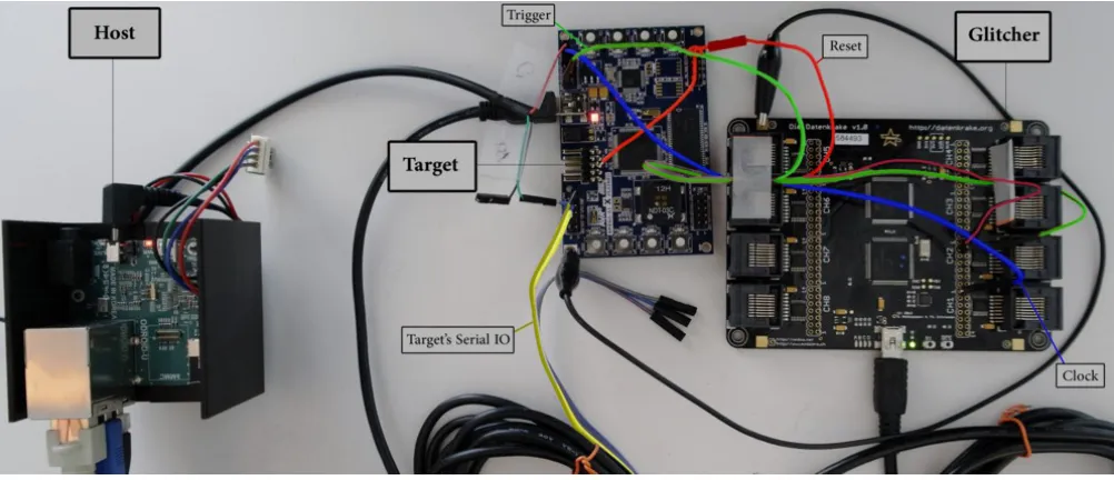
In this section, we detail our general setup for implementing CPU clock glitching. This is the mechanism of altering the code execution by clocking the CPU outside its specification for a short period of time. Our setup is similar to the setup of [36]. It is not specialized to attacks on pairings and can be used in other scenarios. It consists of three main components: the glitcher, the host system, and the target. A block diagram of the setup is shown in Figure 1, and Figure 2 shows a picture of our setup. The glitcher is used to generate the external clock for the target device. It is also used to generate the glitches on the clock signal. The host system is used to configure the glitcher and to acquire the output of the device under attack. The target executes the attacked program. We now describe the three components individually.
Target
Glitcher
*.py
Host
33 MHz 99 MHz Timer
(t_1,d_1,p_1)
(t_2,d_2,p_2)
...
Queue(t_i,d_i,p_i)
*.log CPU
tgt_clk
gl_trig gl_clk
tgt_io gl_cfg
tgt_rst
Figure 1. Simplified block diagram of our setup. The host configures the glitcher, which generates the glitches on the external clock of the target device. The target executes the program under attack.
The glitcher uses two internal clocks: a low frequency clock at fl = 33 MHz and a high frequency clock at fh = 99 MHz. The FPGA implements a32-bit timer that manages the timing of different events. The clock source
of the timer is fl. The glitcher provides a trigger input gl_trig to synchronize it with the target. Internally,
this input is basically used to reset the timer. The main functionality of the glitcher is to generate a clock signal
99 MHz (fh)
33 MHz (fl)
gl_trig
gl_clk
∆
0 1 2 3 4 5 6 7 8 9
t1 d1 t2 d2
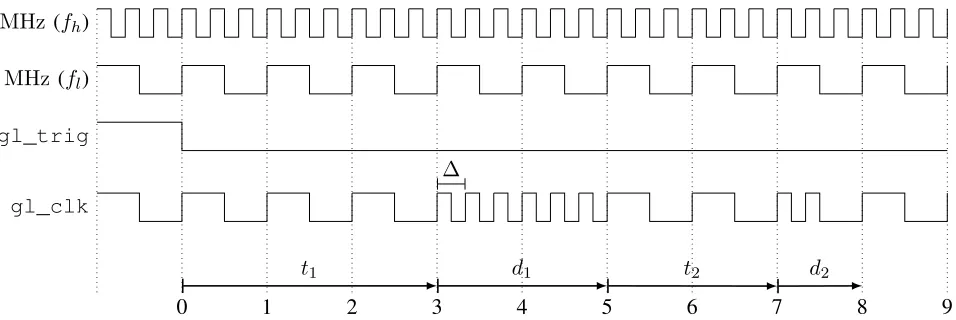
Figure 3. The figure shows the outputgl_clkof the glitcher with two glitches. The first glitch is introduced with a delay oft1= 3 cycles of the33 MHzclock, measured relatively to the trigger gl_trig. Its duration isd1 = 2. With p1 = 1, the99 MHz clock is directly used to generate the glitch pattern. The second glitch is introduced with a delay oft2= 2cycles of the33 MHzclock, measured relatively to the first glitch. Its duration isd2 = 1. Withp2 = 2, the 99 MHzclock is gated in the second half of the33 MHzclock cycle. During a glitch, the delay between two consecutive positive clock edges is∆ = 1/fh.
gl_clk for the target. This output can be switched betweenfl andfh. A glitch is defined by three parameters,
a timestampt, a duration d, and a pattern p. When the timer reachest, a glitch is generated by a synchronized switch fromfl tofh fordperiods offl, i.e.,3·dperiods of fh. We implemented two glitch patterns. Forp= 1,
the high frequency clock fh is directly used to generate the glitch. For p = 2, the clock is gated during the
second half of the fl clock period.
It is crucial for our second-order attack to perform two synchronized glitches. Therefore, the glitcher implements a glitch queue. This queue can be filled with up to 256 triples(t1, d1, p1), . . . ,(t256, d256, p256). Then, for every element in the queue, the corresponding glitch is generated. For second-order attacks only two glitches need to be scheduled in the glitch queue. For more details on how the glitcher works, see [39]. To fill the queue, the glitcher’s internal ARM CPU listens to the serial input at gl_cfg.
Figure 3 shows two glitches. The first glitch is introduced with a delay oft1 = 3cycles of the33 MHzclock, measured relatively to the trigger gl_trig. Its duration is d1 = 2. With p1 = 1, the 99 MHz clock is directly used to generate the glitch pattern. The second glitch is introduced with a delay of t2= 2 cycles of the 33 MHz clock, measured relatively to the first glitch. Its duration is d2 = 1. With p2 = 2, the 99 MHz clock is gated in the second half of the 33 MHz clock cycle. During a glitch, the delay between two consecutive positive clock edges is ∆ = 1/fh.
Host System:The host is a Linux-based system that configures the glitcher and automates the setup. It provides two serial IO lines. One is used to configure the glitcher while the other is used to receive the output from the target. The host system includes a Python [40] library to interface with the glitcher. For example, this allows an in-place analysis and logging of the target’s output, followed by a direct reconfiguration for the next attacks. Another functionality provided by the host is to periodically execute a self-test routine for testing the integrity of the setup.
Target: For an automated reset of the target the glitcher controls the target’s reset pin. Furthermore, the CPU of the target device is clocked with an external clock tgt_clk. We control the CPU clock by connecting tgt_clk to the glitcher output gl_clk.
that initiates the attacked computation.
Finally, the IO of the target is connected to the host for initiating the attacked computation and for analysis of the computation’s results.
B. Instruction Skips
Clock glitches can generate instruction skip faults, instruction replacement faults, and data corruption faults on an AVR CPU [36], which is our target in the concrete attack described in Section V. Introducing faults by clock glitching is done by systematically overclocking the target device at defined instructions. Figure 3 shows a waveform of the target CPU clock. A glitch is introduced at t1 = 3. If the difference ∆ of two consecutive edges is outside of the functional range of the CPU circuit, there is a fair chance that the CPU computation gets disturbed. For example, the opcode of the current instruction may be altered to a non-existing opcode. An AVR CPU ignores invalid opcodes during program execution [36]. This results in instruction skips. Instruction skips by faults can be used to provoke very different effects on the execution of a concrete algorithm. In Section V and Section VI we will show how instruction skips can be used to attack a concrete pairing implementation.
V. SECOND-ORDERFAULTATTACK AGAINST THE ETAPAIRING
This section describes our concrete second-order fault attack against an open source pairing implementation. To conduct the attack, we use the setup that we explained in the previous section. This setup generates the required clock glitches which induce instruction skips.
In Section V-A, we first give an overview how we perform second-order attacks with the setup. We will split the attack into two phases, a profiling phase and a target phase. The profiling phase is only required once. We use it to learn relevant characteristics of the target implementation. Then, in the target phase, the attack can be performed against similar victim devices that store different secrets.
In Section V-B, we introduce our target device and explain our concrete attack on the pairing. Furthermore, we will explain how we were able to break the target implementation in a few minutes for most of the cases. A. Realization of Second-Order Fault Attacks against a Pairing Computation
We use the setup described in Section IV-A. This setup allows us to apply the instruction skip mechanism and log the output of the computation. We place the first fault during the execution of Algorithm 1 such that the cryptanalysis of the Miller inversion will be facilitated. The second fault will be introduced at line 10 to skip the procedure call to the final exponentiation.
To configure the glitcher from Section IV-A, the timing t, the duration d, and the pattern p of the glitches are required. The timing depends on the secret argument of the pairing. Hence, the timing is a priori unknown to us, which makes it challenging to determine t1 and t2. Thus, we execute a profiling phase to find reasonable configurations(t1, d1, p1)and(t2, d2, p2)for the two glitches. We emphasize that once the profiling is completed, we do not need to repeat it when we attack new secrets on similar devices. Without loss of generality, we now assume that the second argumentQ∈G2 is the secret point.
1) Profiling Phase: The profiling relies on two assumptions:
• The assembly code of the target pairing implementation is known to us.
• We are able to execute arbitraryprofiling code on a profiling device similar to the target device.
Based on these assumptions, we first execute a modified pairing implementation on the profiling device. We modify the implementation in one or more of the following ways:
• We are able to compute the pairing for different values of Q that are chosen by us.
• We implement triggers T1 and T2 on two external IO pins. Here, T1 is raised immediately before the first target instruction andT2 is raised immediately before the second target instruction.
These modifications allow us to determine t1 and t2, the timings of the two target instructions, in every computation of the modified pairing. Note thatt2is measured relatively tot1. To measuret2 we use the emulation mode because we are interested in the delay for the case were the first fault has been successful. We execute the modified implementation for different secrets Q chosen uniformly at random from G2. As a result, we obtain distributions fort1 and t2. Since these distributions are obtained over the random choices ofQ, we will choose the parameter triples in the target phase according to them.
These steps of the profiling can be done either by an oscilloscope or by programming a special profiling mode into the FPGA of the glitcher. The profiling mode counts the number of clock cycles between tgt_trig and
T1, and between T1 andT2.
In the next step of the profiling, we determine useful combinations of the remaining glitching parameters d1,
d2,p1, and p2. We do this by performing a large number of experiments where we use the glitcher to introduce glitches at T1 andT2 that are close to the target instructions. We use the fact that we know the values of Q in the profiling phase. Hence, we can predict the output of the algorithm when successfully glitching either one or both of the target instructions. This allows us to identify successful tests and their respective parameters.
2) Target Phase: In the subsequent target phase, the actual target device with the unmodified code and the unknown secret is attacked. Therefore, we perform a sequence of experiments with different combinations of (t1, d1, p1) and (t2, d2, p2) until we are successful in skipping the two target instructions. We select the combinations and their order based on the results of the profiling phase.
B. Realization of our Concrete Second-Order Fault Attack against the eta Pairing
For the concrete pairing implementation we used the RELIC toolkit [23]. It includesCimplementations of finite field arithmetic, ECC, and PBC for different hardware platforms like Atmel’s AVR family. The RELIC toolkit has also been used in TinyPBC for the implementation of PBC in wireless sensor networks [13]. To the best of our knowledge it is the only freely available implementation of PBC for AVR CPUs. In our concrete second-order fault attack, we targeted an AVR XMEGA A1 [41]. AVR controllers are also used in modern smart cards, while our version is freely programmable. A microcontroller from the AVR family was also analyzed in [36]. For our attack, we use RELIC version 0.3.5 without modifications of the source code. We compile the library with the avr-gcc-4.8.2toolchain and optimization level-O11. The RELIC AVR default configuration defines the eta pairing [24] (functionpb_map_etats()) as the standard pairing.
In our experiments both argumentsP andQare loaded from the internal memory. Loading the public argument from memory and not via the serial line helps to simplify the setup, but is not essential for the attack. Then
e(P, Q) is computed on the target device and the output is returned on the serial IO tgt_io.
We placed the first fault at line 9 of Algorithm 1 such that the forloop is terminated after the first iteration. The second fault was introduced at line 10 of Algorithm 1 to skip the procedure call to the final exponentiation. A successful attack gave us a faulty computation where the for loop was executed exactly once and the final exponentiation was not executed at all. In Section VI, we will show how this attack can be analyzed to obtain the secret argument of the pairing. To understand how we attack the end of the for loop, we refer to Table I. It shows how the compiler generates the end of the for loop. An instruction skip fault that removes the rjmp instruction in line 11 causes the loop to terminate immediately. Hence, it realizes our attack that modifies the Miller bound n.
1) Profiling Phase: In the first step, we estimated t1, the clock cycle of the rjmp instruction. Therefore, we executed approximately 32,000 experiments with random choices of Q and measured t1 for each experiment. The distribution oft1 is given in Table II. Then we determined t2, the number of clock cycles from therjmpto the call of the final exponentiation. We used the emulation mode of the profiling code. It allowed us to skip
1
Table I
ASSEMBLY OF END OFF O RLOOP GENERATED WITHA V R-G C C.
3 call fb4_mul_dxs 4 .LVL43:
5 /*decrement loop counter LSB, MSB */ 6 subi r16,1
7 sbc r17,__zero_reg__
8 .loc 1 247 0 discriminator 2 9 breq .+2
10 /*jump to loop begin */ 11 rjmp .L2
12 .LBE2:
13 .loc 1 486 0 14 /* clean stack*/ 15 subi r28,36 16 sbci r29,-2 17 out __SP_L__,r28 18 out __SP_H__,r29 19 pop r29
Table II
DISTRIBUTION OF THE EXECUTION TIMEt1OF THER J M PINSTRUCTION INTABLEI,DEPENDING ON THE INPUTQOFALGORITHM1.
t1 in instruction cycles occurrence in % 422,780 1 <0.01 424,515 1 <0.01 424,941 1 <0.01 427,731 1 <0.01 431,069 1 <0.01
581,804 3 0.01
581,903 28 0.08
582,001 7 0.02
582,002 590 1.66 582,100 30 0.08 582,101 1,763 4.95 582,111 1 <0.01 582,199 297 0.83 582,200 32,890 92.35
the rjmp instruction at t1. We obtained a constant value of t2 = 28. Here, t2 is constant because if the first glitch was successful in leaving theforloop, the code executed between t1 andt2 is independent of the secret. To select combinations ofd1,d2,p1 andp2for the target phase we injected approximately 40,000faults in less than 72 hours. Since we knewQduring profiling, and hence also the values oft1 andt2, we were always able to introduce the faults at the correct instructions. Regarding the two patterns p1 and p2 depicted in Figure 3, both produced good results. To be safe, we propose to use both in the target phase. For the duration of the glitches, we found d1= 3 or d1 = 5 and d2 ≤5 as reasonable settings to use in the target phase.
2) Target Phase: Based on our results from the profiling shown in Table II we scheduledt1 as582,200−i·99 for i∈ {0, . . . ,5}.2 If we did not succeed with one of these values, we fell back to a brute force search with
t1 = 582,200−ifori= 1,2,3, . . . until we were successful. We combined each value oft1 with each combination ofd1,d2,p1, andp2that we determined in the profiling phase. Fort2we added a small safety margin such thatt2 ∈
{26, . . . ,30}. Furthermore, we repeated each combination for 10 times because even with the correct parameters, glitching is not always successful. Hence, for each value of t1 we performed 2·5·2·2·(30−25)·10 = 2,000 experiments. For our setup, one test requires 7.5 seconds on average. This includes configuration of the glitcher, communication from target to host, and self-tests. Hence, we are able to perform more than 10,000 experiments per day.
We will show in Section VI-B that we are able to efficiently determine from the target’s output whether both instruction skips were successful or not. Furthermore, we will show that for a successful attack, we are able to efficiently compute the secret Q. Hence, once we detected the first successful experiment, we discarded all remaining experiments to start the next attack.
We repeated the attack for five different secrets, drawn uniformly at random from G2. We were always successful in skipping both instructions. The analysis of the experiments showed that for all secrets it occurred thatt1 was either582,200or582,101. This is in line with the distribution in Table II. Hence, for each attack we required at most 2·2,000 experiments, whereas in the cases with t1 = 582,200, much fewer experiments were required and it took us only minutes to be successful.
VI. ANALYSIS OFFAULTYCOMPUTATIONS
We now resume the description of the second-order fault attack by explaining the mathematical analysis which leads from the faulty computation to the secret key. We will first provide mathematical details of the attacked implementation and then give two examples, one for each category from Section III. With our setup from Section IV, we can realize any fault from both categories, i.e., all theoretical faults that have been presented so far. However, we concentrate on two examples to illustrate both categories.
The first example is the concrete attack from Section V. It illustrates the modification of the Miller loop bound
n. The second example illustrates the modification of the Miller variable f. Both these analyses have already been described similarly, cf. [15], [20], [21], [33]. In both examples, we assume to know P = (xP, yP), while Q = (xQ, yQ) is secret. We induce the first fault during the computation of the Miller Algorithm and use the
second fault to skip the function call to the final exponentiation. Thus, we do not have to solve the exponentiation inversion, but only a facilitated Miller inversion.
A. Mathematical Details of the Attacked Implementation
We attacked an implementation of the eta pairing in characteristic 2 on supersingular elliptic curves. We decided to attack the eta pairing [24] despite current research results which indicate that it should no longer be used for security applications, cf. [25], [26]. This was due to the fact that the eta pairing is the default for AVR devices in the attacked RELIC library [23]. However, the attack can be easily applied to other pairings. The concrete implementation is very similar to the implementation proposed in [24, Section 6] and is presented in Algorithm 2. The elliptic curve E : y2 +y = x3 +x is defined over the finite field Fq with q = 2m and m = 271 in
our implementation. For our case, i.e., m = 7 mod 8, it holds that #E(Fq) = 2m+ 2(m+1)/2+ 1. We define
the extension field Fq4 =Fq(s, t) of degree 4, with s2 =s+ 1 and t2 = t+s. Let z = (q4 −1)/#E(Fq) = (22m−1)·(2m−2(m+1)/2+ 1),n= 2(m+1)/2+ 1, andψ(x,y) = (x+ 1 + 1, y+sx+t). For inputP, Q∈E(Fq)
the eta pairing η is then defined as
η(P, Q) =fn,−P(ψ(Q))z.
Because of the simple binary form of n, the main loop of Algorithm 1 mainly reduces to point doubling and squaring of field elements in Fq4, followed by one multiplication with l[2(m+1)/2](−P),−P(ψ(Q)) for the least
significant bit of n. As in [24, Algorithm 3], the eta implementation computes the loop in reversed order in the RELIC library [23]. Therefore, P0 =
2(m−1)/2)
unrolled:
fn,−P(ψ(Q)) =l[2]P0,−P(ψ(Q))·gP0(ψ(Q))· (m−1)/2
Y
j=1
g[2−j]P0(ψ(Q))2
j
. (1)
Algorithm 2 Implementation ofη(P, Q) on E(F2m) for m= 7 mod 8 andE :y2+y =x3+x.
Require: P = (xP, yP), Q= (xQ, yQ)∈E
Ensure: η(P, Q)
1: u←xP, v←xQ
2: g←u·v+yP +yQ+ 1 + (u+xQ)s+t
3: u←x2P
4: l←g+v+u+s
5: f ←g·l
6: fori= 1 .. (m−1)/2 do 7: xQ←xQ2, yQ←yQ2
8: xP ←
√
xP, yP ←
√
yP
9: u←xP, v ←xQ
10: g←u·v+yP +yQ+ 1 + (u+xQ)s+t
11: f ←f·g
12: end for 13: f ←fz
14: return f
Algorithm 2 shows how the computation of (1) is implemented in the RELIC library. B. Example: Analysis after Modification of n
Now, we analyze the output of our second-order attack from Section V. For the concrete RELIC implementation, the two instruction skip faults target the first execution of line 12 and the execution of line 13 of Algorithm 2. Hence, Table I shows the generated assembly for line 12 of Algorithm 2.
In an execution were both fault injections are successful, the forloop is executed exactly once and the final exponentiation is completely skipped. Since one loop is unrolled, this corresponds to an execution with two iterations of the loop in Algorithm 1, and a modification ofnfrom2(m+1)/2+ 1to22+ 1. We see that our attack is in the category of faults that modify n. Let α be the output of the faulty computation fn,P0 (ψ(Q)). With (1) we obtain
α=fn,0 −P(ψ(Q)) =l[2]P0,−P(ψ(Q))·gP0(ψ(Q))·
g[2−1]P0(ψ(Q))2.
(2)
The following steps describe how we recover the secret input Qof Algorithm 2 from α.
1) Algebraic Model of the Secret: First, we define variables x and y representing thex-coordinate and the
y-coordinate of the secret Q. Now we describe Q as the root of a rational function. With (2) we define
fP(x,y) :=fn,0 −P(ψ(x,y))−α. (3)
Sincefn,0 −P(ψ(x,y)) is a product of four lines, fP(x,y) is of degree at most 4 inx andy. In our case the
secret is already defined over the strict subfield Fq of Fq4. We model this by considering Fq4 as an k= 4
dimensional vector space over Fq. Then (3) can be re-written as four individual polynomials fP(1), . . . ,fP(4)
2) Computation of Candidates: At this point, we define the variety VQ = V
fP(1), . . . , fP(4)
∩ E by a (possibly overdetermined) system of nonlinear multivariate equations. Since Q∈VQ, we now compute all elements of VQ in this step. The complexity of this step mainly depends on the degrees of f
(1)
P , . . . , f
(4)
P
and is reduced by using more equations than variables.
3) Testing Candidates:In the final step, we identify the secret from all elements inVQ. To do this, we compute η(P, Q0) for the elements Q0 ∈VQ. Each result is compared with η(P,Q) that has been obtained from an
error-free execution to identify the unique point Q.
Note that the case where P is the secret can be handled analogously. The major difference is that we replace
fP(x,y) from step 1 by a polynomial where x and y represent
√
xP and
√
yP. From Algorithm 2 we see that
the degree offP(x,y)will now become at mostd= 7. Due to the higher degree, the analysis will become more
expensive.
Note that restricting to subfields as in step 1 can often be exploited. For example, it has been used in [21] and [32]. Indeed, the most common optimization for the implementation of pairings is to choose the first argument
P in G1 ⊆ E(Fq). Furthermore, for Type 1 pairings the second argument Q is also Fq-rational. For Type 3
pairings, Qis defined in G2 ⊆E0(Fqk0) where E0 is a degree k0 twist of E and k0 divides k. For details on the
selection of pairing-friendly curves we refer to [42].
As explained in Section V, many experiments fail in delivering the intended faults, i.e., in simultaneously skipping both target instructions. For a failed experiment, no candidate Q0 will pass step 3. Hence, in practice it is crucial to automate step 2 and step 3 for identifying the first successful experiment. We automated the analysis based on Sage [43], a free computer algebra system. Therefore, we re-implemented the eta pairing from the RELIC library in Sage. This implementation allows us to compute the pairing on arbitrary inputs P, Q, andn. Based on this implementation, we are able to automatically construct the multivariate polynomial (3) from step 1 for any value α. Step 2 is an invocation of the variety() function on the ideal generated by fP(1), . . . ,fP(4)
and y2+y =x3+x. This computation is based on Gr¨obner basis techniques. Hence, using five equations for only two variables accelerates this step. Finally, in step 3 we use the implementation of the pairing again, but evaluate it at the candidate points Q0 to identifyQ.
Our non-optimized implementation requires less than one second for processing one faulty output α. This is less time than the target device requires to compute the pairing. Hence, the mathematical computation is not critical for the performance of our attack.
C. Example: Analysis after Modification of f.
For this example, we attack two computations of η(P, Q). In both computations, the same input has to be used. During the first computation, we only use one fault and skip the final exponentiation. We denote the output with α1, i.e., α1 =fn,−P(ψ(Q)). In the second computation, we also skip the final exponentiation. Prior to this
fault, we induce another fault to skip an instruction which is involved in the update of the Miller variable f. In the general description of the Miller Algorithm, this corresponds to the lines 3, 4, 6 or 7 of Algorithm 1. In our concrete implementation, cf. Algorithm 2, also several instructions can be skipped to achieve a modification of
f. For this example, we choose to illustrate the modification off by skipping the update ofu once. Thus, either line 3 or line 9 in any round of the for loop in Algorithm 2 can be skipped. We choose to skip line 3. We denote the second faulty output with α2, i.e., α2 = fn,0 −P(ψ(Q)). Since α1 and α2 are known, we also know
α=α1/α2∈Fq4.
1) Algebraic Model of the Secret:The two valuesα1 andα2 have the same first factorg, which is computed in line 2, but differ in their factorl, which depends onu. Since u depends on xP afterwards, which is not
are equal. Thus, since all but the respective factors l ofα1 andα2 are equal, we receive the equation
xP ·xQ+yP +yQ+ 1
+ (xP +xQ)·s+t+xQ+x2P +s =α·[xP·xQ+yP +yQ+ 1
+ (xP +xQ)·s+t+xQ+xP +s],
(4)
with all values except xQ andyQ known.
2) Computation of Candidates: The elliptic curve is defined by E :y2+y =x3+x. It gives us a second equation with root Q. By writing both E and (4) as univariate polynomials in y and using the theory of resultants, we get a univariate polynomial inx which has degree at most 3.
Res(α·fn,0 −P(ψ(x, y))−fn,−P(ψ(x, y)), E) = (α−1)2·(−x3−x)
+h(α−1)(xP·x+xP +x+yP + 1
+ (xP +x+ 1)·s+t)−x2P +xP
i2
−h(α−1)(xP·x+xP +x+yP + 1 + (xP +x+ 1)·s+t)−x2P +xP
i
·(α−1)
(5)
All roots of this polynomial are candidates forxQ. For each of these candidates we evaluateE and thereby
get two candidates for the secret point Q.
3) Testing Candidates:Since we know the concrete implementation, we now computeη(P, Q0) for all candi-datesQ0 and compare the results withη(P, Q), which has been obtained from an error-free execution. Since Equation 5 has degree at most 3 andE has degree 2 iny, we have to test at most six candidates to identify the unique point Q.
Note that again, the roles of xQ andyQ can be switched. The resulting univariate polynomial iny has at most
degree 4, and we will then get three candidates for the secret point for each root. Thus, we have to test at most twelve candidates.
VII. CONCLUSION
Several fault attacks against pairing-based cryptography have been published in the past. Interestingly, none of these have been practically evaluated. We accomplished this task and proved that fault attacks against pairing-based cryptography are indeed possible and are even practical — thus posing a serious threat. Moreover, we successfully conducted a practical second-order fault attack against an open source implementation of the eta pairing on an AVR XMEGA A1. We used this freely programmable chip to validate our attacks on a real-world smart card platform. On the basis of a new two-part categorization of all conceivable fault attacks against the underlying Miller Algorithm, we were able to reveal the secret point of a pairing in both categories.
— after almost 20 years of intensive research — it is natural that the young field of pairing-based cryptography requires more research after our successful attack.
ACKNOWLEDGMENT
J. K. gratefully acknowledges support by the Deutsche Telekom Stiftung. We thank Universidade Federal do Rio Grande do Sul and Technische Universit¨at Berlin for allowing R.G.d.S. to do a dual-degree program. We also thank our colleague Dmitry Nedospasov who supported this work with productive ideas for the glitcher development.
REFERENCES
[1] D. Boneh, R. A. DeMillo, and R. J. Lipton, “On the Importance of Checking Cryptographic Protocols for Faults,” in
EUROCRYPT’97, ser. Lecture Notes in Computer Science, vol. 1233. Springer Berlin Heidelberg, 1997, pp. 37–51.
[2] I. Verbauwhede, D. Karaklajic, and J.-M. Schmidt, “The Fault Attack Jungle - A Classification Model to Guide You,” inFDTC, 2011, pp. 3–8.
[3] H. Bar-El, H. Choukri, D. Naccache, M. Tunstall, and C. Whelan, “The Sorcerer’s Apprentice Guide to Fault Attacks,”
Proceedings of the IEEE, vol. 94, no. 2, pp. 370–382, Feb 2006.
[4] C. Kim and J.-J. Quisquater, “Fault Attacks for CRT Based RSA: New Attacks, New Results, and New Countermea-sures,” inInformation Security Theory and Practices. Smart Cards, Mobile and Ubiquitous Computing Systems, ser. Lecture Notes in Computer Science, 2007, vol. 4462, pp. 215–228.
[5] E. Dottax, C. Giraud, M. Rivain, and Y. Sierra, “On Second-Order Fault Analysis Resistance for CRT-RSA Implementations.” inWISTP, ser. Lecture Notes in Computer Science, vol. 5746. Springer Berlin Heidelberg, 2009, pp. 68–83.
[6] A. Menezes, S. Vanstone, and T. Okamoto, “Reducing Elliptic Curve Logarithms to Logarithms in a Finite Field,” in
Proceedings of the Twenty-third Annual ACM Symposium on Theory of Computing, ser. STOC ’91, 1991, pp. 80–89.
[7] D. Boneh and M. Franklin, “Identity-Based Encryption from the Weil Pairing,” SIAM J. of Computing, vol. 32, no. 3, pp. 586–615, 2003, extended abstract in Crypto’01.
[8] A. Shamir, “Identity-based Cryptosystems and Signature Schemes,” in Advances in Cryptology - CRYPTO 84, ser. Lecture Notes in Computer Science, vol. 196. Springer-Verlag New York, Inc., 1985, pp. 47–53.
[9] D. F. Aranha, P. S. L. M. Barreto, P. Longa, and J. E. Ricardini, “The realm of the pairings,” in Selected Areas in Cryptography, ser. Lecture Notes in Computer Science, vol. 8282. Springer Berlin Heidelberg, 2013, pp. 3–25.
[10] A. Sahai and B. Waters, “Fuzzy Identity-based Encryption,” in EUROCRYPT 2005, ser. Lecture Notes in Computer Science, vol. 3494. Springer Berlin Heidelberg, 2005, pp. 457–473.
[11] F. Hess, “Efficient Identity Based Signature Schemes Based on Pairings,” inSAC 2002, LNCS 2595. Springer Berlin Heidelberg, 2002, pp. 310–324.
[12] A. Joux, “A One Round Protocol for Tripartite Diffie-Hellman,” in Proceedings of the 4th International Symposium on Algorithmic Number Theory, ser. ANTS-IV. Springer Berlin Heidelberg, 2000, pp. 385–394.
[14] L. B. Oliveira, D. F. Aranha, E. Morais, F. Daguano, J. L´opez, and R. Dahab, “TinyTate: Identity-Based Encryption for Sensor Networks,”IACR Cryptology ePrint Archive, 2007.
[15] D. Page and F. Vercauteren, “A Fault Attack on Pairing-Based Cryptography,” IEEE Transactions on Computers, vol. 55, no. 9, pp. 1075–1080, 2006.
[16] S. D. Galbraith, F. Hess, and F. Vercauteren, “Aspects of Pairing Inversion,”IEEE Transactions on Information Theory, vol. 54, no. 12, pp. 5719–5728, 2008.
[17] N. Kanayama and E. Okamoto, “Approach to Pairing Inversions Without Solving Miller Inversion,”IEEE Transactions on Information Theory, vol. 58, no. 2, pp. 1248–1253, 2012.
[18] I. Biehl, B. Meyer, and V. M¨uller, “Differential Fault Attacks on Elliptic Curve Cryptosystems,” in Advances in Cryptology — CRYPTO 2000, ser. Lecture Notes in Computer Science, vol. 1880, 2000, pp. 131–146.
[19] S. D. Galbraith, Mathematics of Public Key Cryptography. Cambridge University Press, 2012.
[20] N. E. Mrabet, “What about Vulnerability to a Fault Attack of the Miller’s Algorithm During an Identity Based Protocol?” inProceedings of the 3rd International Conference and Workshops on Advances in Information Security and Assurance, ser. ISA ’09. Springer Berlin Heidelberg, 2009, pp. 122–134.
[21] C. Whelan and M. Scott, “The Importance of the Final Exponentiation in Pairings When Considering Fault Attacks,” inPairing, ser. Lecture Notes in Computer Science, vol. 4575. Springer Berlin Heidelberg, 2007, pp. 225–246.
[22] R. Lashermes, J. Fournier, and L. Goubin, “Inverting the Final Exponentiation of Tate Pairings on Ordinary Elliptic Curves Using Faults,” inCHES, ser. Lecture Notes in Computer Science, vol. 8086. Springer Berlin Heidelberg, 2013, pp. 365–382.
[23] D. F. Aranha and C. P. L. Gouvˆea, “RELIC is an Efficient LIbrary for Cryptography,” http://code.google.com/p/ relic-toolkit/.
[24] P. S. L. M. Barreto, S. D. Galbraith, C. O’Eigeartaigh, and M. Scott, “Efficient pairing computation on supersingular abelian varieties,”Des. Codes Cryptography, vol. 42, no. 3, pp. 239–271, 2007.
[25] R. Granger, T. Kleinjung, and J. Zumbragel. (2014) Discrete Logarithms in the Jacobian of a Genus 2 Supersingular Curve over GF(2367). Accessed: 2014-01-30. [Online]. Available: https://listserv.nodak.edu/cgi-bin/wa.exe?A2=
NMBRTHRY;23651c2.1401
[26] G. Adj, A. Menezes, T. Oliveira, and F. Rodr´ıguez-Henr´ıquez, “Computing Discrete Logarithms inF36∗137 andF36∗163
using magma,”IACR Cryptology ePrint Archive, 2014.
[27] R. Barbulescu, P. Gaudry, A. Joux, and E. Thom´e, “A heuristic quasi-polynomial algorithm for discrete logarithm in finite fields of small characteristic,” in EUROCRYPT 2014, ser. Lecture Notes in Computer Science, vol. 8441. Springer Berlin Heidelberg, 2014, pp. 1–16.
[28] V. S. Miller, “The weil pairing, and its efficient calculation,”J. Cryptology, vol. 17, no. 4, pp. 235–261, 2004.
[29] M. Joye and G. Neven, Eds.,Identity-based cryptography, ser. Cryptology and Information Security Series. IOS Press, 2008.
[31] I. F. Blake, G. Seroussi, and N. P. Smart, Eds.,Advances in Elliptic Curve Cryptography, ser. London Mathematical Society Lecture Note Series. Cambridge University Press, 2005, no. 317.
[32] F. Vercauteren, “The Hidden Root Problem,” in Proceedings of the 2nd international conference on Pairing-Based Cryptography, ser. Pairing ’08. Springer Berlin Heidelberg, 2008, pp. 89–99.
[33] N. E. Mrabet, D. Page, and F. Vercauteren, “Fault Attacks on Pairing-Based Cryptography,” in Fault Analysis in Cryptography. Springer Berlin Heidelberg, 2012.
[34] K. Bae, S. Moon, and J. Ha, “Instruction Fault Attack on the Miller Algorithm in a Pairing-Based Cryptosystem,” in
IMIS. IEEE, 2013, pp. 167–174.
[35] D. Page and F. Vercauteren, “Fault and Side-Channel Attacks on Pairing Based Cryptography,”IACR Cryptology ePrint Archive, 2004.
[36] J. Balasch, B. Gierlichs, and I. Verbauwhede, “An In-depth and Black-box Characterization of the Effects of Clock Glitches on 8-bit MCUs,” inFDTC, 2011, pp. 105–114.
[37] ODROID-U2 Product Page. Accessed: 2014-05-29. [Online]. Available: http://hardkernel.com/main/products/prdt info.php?g code=G135341370451
[38] D. Nedospasov and T. Schroder, “Introducing Die Datenkrake: Programmable Logic for Hardware Security Analysis,” in7th USENIX Workshop on Offensive Technologies, 2013.
[39] R. G. da Silva, “Practical Analysis of Embedded Microcontrollers against Clock Glitching Attacks,” Bachelor’s Thesis, Technische Universit¨at Berlin, 2014.
[40] Python Programming Language Homepage. Accessed: 2014-05-15. [Online]. Available: http://www.python.org
[41] ATxmega128A1 Product Page. Accessed: 2014-05-21. [Online]. Available: http://www.atmel.com/devices/ atxmega128a1.aspx
[42] P. S. L. M. Barreto, B. Lynn, and M. Scott, “On the Selection of Pairing-Friendly Groups,” in Selected Areas in Cryptography, ser. Lecture Notes in Computer Science, vol. 3006. Springer Berlin Heidelberg, 2003, pp. 17–25.
[43] W. A. Stein. (2014) Sage Mathematics Software (Version 6.1). [Online]. Available: http://www.sagemath.org