arXiv:physics/0206028v1 [physics.atom-ph] 11 Jun 2002
potential
C. Figueira de Morisson Faria,1 H. Schomerus,2 and W. Becker1,∗ 1
Max-Born-Institut, Max-Born-Str. 2a, 12489 Berlin, Germany
2Max-Planck Institut f¨ur Physik komplexer Systeme, N¨othnitzer Str. 38, 01187 Dresden, Germany
(Dated: February 2, 2008)
A versatile semiclassical approximation for intense laser-atom processes is presented. This uniform approxi-mation is no more complicated than the frequently-used multi-dimensional saddle-point approxiapproxi-mation and far superior, since it applies for all energies, both close to as well as away from classical cutoffs. In the latter case, it reduces to the standard saddle-point approximation. The uniform approximation agrees accurately with numeri-cal evaluations for potentials, for which these are feasible, and constitutes a practicable method of numeri-calculation in general. The method is applied to the calculation of high-order above-threshold ionization spectra with various binding potentials: Coulomb, Yukawa, and shell potentials which may model C60molecules or clusters. The shell potentials generate high-order ATI spectra that are more structured and may feature an apparently higher cutoff.
I. INTRODUCTION
Sufficiently intense laser fields ionize atoms or molecules by the quantum-mechanical process of tunneling [1]. Both the tunneling process and the ensuing motion of the electron in the continuum are well accessible to semiclassical meth-ods. Tunneling generates a wave packet whose center follows a classical trajectory while the wave packet is spreading. It may or may not return to within the range of the ionic bind-ing potential. If it does, the well-known recollision-induced processes, such as high-order harmonic generation (HHG) or high-order above-threshold ionization (ATI), take place [2, 3].
In the tunneling regime, the quantum-mechanical transition amplitude can be analyzed, computed, and interpreted via the saddle-point approximation [4, 5]. Typically, the transition amplitude is represented by a multi-dimensional integral over the timet′
at which the electron enters the continuum by tun-neling, the later timet at which it revisits the ion, and one or all components of the drift momentumk along its orbit in between those two times. For a specified final state, e.g., for given final momentum of the electron after the recollision or for given frequency of high-order harmonic emission, the saddle-point approximation selects those particular “quantum orbits” that contribute to this final state. These orbits are char-acterized by particular values of the parameterst, t′
andk, which are complex numbers because of the tunneling nature of these orbits. For a specified final state, there are, in general, several contributing quantum orbits. Their contributions have to be added coherently, and this yields an interference pattern, which may appear very intricate, even though its physical ori-gin is simple [6, 7].
Within the context of atoms in strong fields, the contribut-ing quantum orbits typically come in pairs. This may be best known from the Lewenstein model of HHG: For specified harmonic order within the “plateau”, there are two quantum
∗also at Center for Advanced Studies, Department of Physics and Astronomy,
University of New Mexico, Albuquerque, NM 87131
orbits whose contributions dominate the harmonic yield, the “long orbit” and the “short orbit”. An electron on the long orbit starts earlier (by ionization) and returns later (for recom-bination) than an electron on the short orbit [4]. This is a very general feature of intense-laser–atom processes and holds also for the more complicated orbits, which bypass the ion once or several times before the recombination process takes place [6]. For fixed laser intensity, the maximal HHG frequency or the maximal energy of an ATI electron obey classical lim-its [2, 8], which are related to the maximal kinetic energy of the electron returning to the ion. For parameters approaching such classical limits, the two quantum orbits become more and more identical. If it were not for the fact that their parameters are complex, reflecting the birth of the electron by tunneling, the two orbits of a pair would coalesce at the classical cutoff [6].
action and its second derivative at the saddle points. Problem (i) is solved because the uniform approximation regularizes the saddle-point integrals close to the classical cutoff, while it reduces to the saddle-point approximation far away from the cutoff. Problem (ii) is solved by imposing the simple re-quirement of continuity on the transition amplitude, which automatically selects the appropriate branch of the multival-ued solution that does not contain the contribution of the un-physical saddle point beyond the classical cutoff. For a zero-range binding potential, the benefit of the saddle-point ap-proximation lies in the insight gained by the introduction of a few quantum orbits, which allow one to visualize the physi-cal mechanism behind recollision-induced processes. For the mere purpose of computation, the transition amplitude can be calculated as well, if not more easily, via a simple quadrature. We will use the zero-range potential as a test case, and find ex-cellent agreement for the uniform approximation, even where the usual saddle-point approximation fails.
The zero-range potential is a valid model for the descrip-tion of a negatively charged ion in an intense laser field [14, 15, 16]. To what extent it can also be employed to model an atom in an intense laser field or, in other words, just how important the long range of the Coulomb potential is in this situation, has been the object of some debate. Sur-prisingly, it has turned out that at least for the qualitative ex-planation of most intense-field effects the Coulomb tail is not instrumental [4, 5, 17]. Still more surprisingly, even the sub-tle quantum-mechanical enhancements of the ATI plateau at certain sharply defined intensities [18] are not specific to the Coulomb potential. In fact, a zero-range potential yields vir-tually the same enhancements, though at slightly different in-tensities [19].
From this point of view, being able to compare ATI spectra from zero-range and non-zero-range potentials is important. However, for non-zero-range potentials, a direct computation of the transition amplitude requires one to carry out a cumber-some multidimensional integral, and the uniform saddle-point approximation is the only viable approach.
The purpose of this paper then is twofold. First, we deter-mine the specific uniform approximation that applies to the pairs of quantum orbits that appear in laser-induced rescatter-ing processes. Second, we use this uniform approximation to investigate the influence of the form of the binding potential on ATI.
The plan of the paper is as follows: In Sec. II, we sum-marize the improved Keldysh approximation for the transition amplitude. In Sec. III, we discuss the saddle points that feature in the saddle-point approximation as well as in the uniform approximation, and review the saddle-point approximation as well as its problems close to classical cutoffs. In Sec. IV, we determine the uniform approximation that overcomes these problems and describe its conceptual relation to the saddle-point approximation. In Sec. V we compare the ATI spec-tra obtained by these approximations to the numerical results for the zero-range binding potential. The uniform approxima-tion is then used in Sec. VI to address the effect of a general (non-zero-range) binding potential on the ATI spectrum, us-ing Coulomb, Yukawa, and shell potentials as examples. A
summary of the results and conclusions can be found in Sec. VII.
We use atomic units (a.u.) throughout this paper.
II. TRANSITION AMPLITUDE FOR RESCATTERING PROCESSES
Strong-field phenomena, such as above-threshold ioniza-tion (ATI), are successfully described by transiioniza-tion amplitudes derived within a framework known as the strong-field approx-imation. This approximation neglects the binding potential in the propagation of the electron in the continuum, and the laser field when the electron is bound, which corresponds to treat-ing the process of rescattertreat-ing in the first-order Born approx-imation on the background of the laser field. (The first-order Born approximation yields the exact differential cross section in the absence of the field both for the Coulomb potential as well as for the zero-range potential.) The ATI transition am-plitude for the direct electrons – electrons that leave the vicin-ity of the ion right after they have tunneled into the continuum – is the well-known Keldysh-Faisal-Reiss (KFR) amplitude [20]
Mdir=−i
Z ∞
−∞
dt′hψp(V)(t ′
)|V|ψ0(t′)i. (1)
The generalized transition amplitude, which includes one sin-gle act of rescattering, is given by [21]
Mresc=−
Z ∞
−∞
dt
Z t
−∞
dt′
hψp(V)(t)|V U (V)(t, t′
)V|ψ0(t′)i.
(2)
In both equations, V denotes the atomic binding potential, the final state is the Volkov state describing a charged parti-cle with asymptotic momentumpin the presence of a field with vector potentialA(t),
hr|ψ(pV)(t)i= exp
−2i
Z ∞
t
dτ[p+A(τ)]2
ei[p+A(t)]·r,
(3)
andU(V)(t, t′
)is the Volkov time-evolution operator, which describes the evolution of the electron in the presence of only the laser field. In Eq. (1), the electron, initially in the ground state|ψ0(t′)i, is ionized into its final state at the timet′. In
Eq. (2), an additional rescattering off the binding potential at the timet is accounted for. The amplitude (2) incorporates the amplitude (1) for direct ionization in the limit wheret′
→ t. Hence, the two amplitudes must not be added [21]. The amplitude (2) or closely related versions thereof have been used by several authors [9, 10, 22, 23].
If we insert the expansion of the Volkov propagator in terms of Volkov states,
U(V)(t, t′
) =
Z
d3k|ψ(kV)(t)ihψk(V)(t′
into Eqs. (1) and (2), the transition amplitudes can be rewritten as
Mdir=−i
Z ∞
−∞
dt′
exp[iSp(t′)]Vp0, (5)
and
Mresc=−
Z ∞
−∞
dt
Z t
−∞
dt′
Z
d3keiSp(t,t′,k)V
pkVk0, (6)
where the corresponding actions are given by
Sp(t′) =− 1 2
Z ∞
t′
dτ [p+A(τ)]2+|E0|t (7)
and
Sp(t, t′,k) = − 1 2
Z ∞
t
dτ [p+A(τ)]2
− 12
Z t
t′
dτ [k+A(τ)]2+|E0|t′. (8)
The quantity|E0|denotes the ionization potential of the atom.
In this paper, we address the case of a linearly polarized monochromatic field,
A(t) =A0excosωt, (9)
with the ponderomotive energyUP =hA2(t)it/2 =A20/4.
The representations (5) and (6) are particularly useful if the form factors
Vpk = hp+A(t)|V |k+A(t)i
= 1 (2π)3
Z
d3r exp[−i(p−k)·r]V(r) (10)
and
Vk0 = hk+A(t′)|V|0i
= 1
(2π)3/2
Z
d3rexp[−i(k+A(t′))·r]V(r)ψ0(r)
(11)
can be calculated in analytical form. Within the strong-field approximation, the influence of the binding potential is en-tirely contained in these two matrix elements. For a zero-range potential, the form factors are constants. In this case, the five-dimensional integral (6) can be reduced to a one-dimensional integral over a series of Bessel functions, which can be readily computed numerically [21, 24]. In Sec. V, we will refer to the outcome of this procedure as the “exact re-sult”. In general, however, a correspondingly “exact” evalua-tion of the matrix element (2) has to deal with a multidimen-sional integral.
III. SADDLE-POINT ANALYSIS
For sufficiently high intensity of the laser field, correspond-ing to small Keldysh parameterγ =p
|E0|/2UP, ionization
can be envisioned to proceed via the quasistatic process of tunneling [25]. The transition amplitudes (5) and (6) are then conveniently computed via the method of steepest descent. Both the standard saddle-point approximation as well as the uniform approximation rest on this method, which approxi-mates the entire integral by the contributions from the vicinity of those points on the integration contour where the action is stationary, i.e., where the partial derivatives of the action with respect to the integration variables vanish. These points correspond to maxima of the integrand after a deformation of the original integration manifold, which is constructed such that the integrand decreases roughly like a Gaussian when one moves away from the vicinity of the saddles [11].
In the current section, we first write down the equations that determine the saddle points, then describe the general proce-dure of identifying the relevant saddles, and finally discuss the saddle-point approximation. All these items are prerequisites for the discussion of the uniform approximation in Sec. IV.
A. Saddle-point equations
For the rescattering amplitude (6), the saddle-point equa-tions are
[k+A(t′)]2 = −2|E0|, (12)
[p+A(t)]2 = [k+A(t)]2, (13)
Z t
t′
dτ[k+A(τ)] = 0. (14)
Their solutions determine the ionization timet′
, the rescatter-ing timet, and the drift momentumkof the electronic orbit in between those two times, such that the electron acquires the asymptotic momentump. Equations (12) and (13) are related to energy conservation at the ionization time and the rescat-tering time, respectively, and Eq. (14) determines the interme-diate electron momentum. For the direct amplitude (5), only the ionization timet′ need be determined, and the resulting
equation is like Eq. (12) withk replaced by the asymptotic momentump.
Evidently, Eq. (12) has no real solutions t′
as long as E0 6= 0, and in consequencet, t′ andkare complex.
Phys-ically, the fact thatt′ is complex means that ionization takes
place through a tunneling process. The solutions(t, t′
)of the saddle-point equations for the linearly polarized monochro-matic field (9) have been computed in Ref. [6]. They only depend on the ionization energyE0 and the photoelectron
momentump, but not on the shape of the binding potential, which enters the transition amplitude only via the form factors (10) and (11).
A very important feature of the solutions is that they come in pairs. Let us denote the “travel time” byτ ≡t−t′. Then,
B. Classical cutoffs and Stokes transitions
The original contour of integration in the amplitudes (5) or (6) is along the real axes, while the solutions of the saddle-point equations (12)–(14) are located off the real axes in the complex plane. A central question in the method of steepest descent then is, which of the various saddle points are vis-ited by the steepest-descent integration manifold. We shall call those the relevant saddle points. The steepest-descent manifold consists of pieces with a constant real part of the action. These pieces are glued together at zeros of the inte-grand, at which the phase of the action is not well defined. Usually, each piece visits only a single saddle point, which also determines the constant real part of the action. Only such pieces that are needed to connect the integration boundaries give contributions to the transition amplitude. The number of these pieces can change in a so-called Stokes transition, when two pieces merge at a certain value of a parameter (here we consider the photoelectron momentump). On either side of the Stokes transition, the manifolds of the saddles of interest are glued together in different ways: on one side, both pieces are needed to connect the integration boundaries (plus, pos-sibly, other pieces related to different pairs of saddle points), while only one of the pieces is needed on the other. Note that in the latter case, too, there are still two solutions of the saddle-point equations, but only one of them is visited by the steepest-descent deformation of the original integration man-ifold [26].
Merging of steepest-descent manifolds requires that the real parts of the actions of two quantum orbits become identical at a specific value ofp,
ReSp(ti, t′i,ki) = ReSp(tj, t′j,kj), (15)
whereiandj denote the saddle points of the given pair, and the timestsandt′s(s = i, j)depend onp. It follows from the physical mechanism behind high-order ATI that both sad-dles of each pair are relevant provided the asymptotic mo-mentum is classically accessible. For the pair of orbits hav-ing the shortest travel times (n = 1), this is the case if
p2/2≤10.007UP[27]. The other pairs of orbits have smaller cutoff energies.
The relevant saddle beyond the classical cutoff is the one that has the smaller imaginary part of the action at the Stokes transition [28]. In the following we reserve the indexi for this saddle. Saddlejonly maintains a residual contribution to the transition amplitude after the Stokes transition, until it be-comes completely irrelevant in the so-called anti-Stokes tran-sition
ImSp(ti, t′i,ki) = ImSp(tj, t′j,kj). (16)
The anti-Stokes transition coincides with the Stokes transition if both saddles actually coalesce. Otherwise, it frequently oc-curs very shortly after the Stokes transition.
Exactly how the transition amplitude behaves close to the classical cutoff can only be described when the interplay of both saddles is taken into account in a systematic way, which is achieved by the uniform approximation. Before we turn to
this approximation, we now discuss the standard saddle-point approximation.
C. Saddle-point approximation
Within the saddle-point approximation, the amplitudes (5) and (6) are approximated by
Mdir(SPA)=X s
s
2πi ∂2S
p/∂t2s
Vp0exp[iSp(ts)] (17)
and
M(SPA) resc =
X
s
Asexp(iSs), (18a)
Ss = Sp(ts, t′s,ks), (18b)
As = (2πi)5/2q VpksVks0
detS′′
p(t, t′,k)|s
, (18c)
respectively, where the indexsruns over the relevant saddle points, andS′′
p(t, t
′,k)
|sis the five-dimensional matrix of the second derivatives of the action (8) evaluated at the solutions of the saddle-point equations (12)-(14).
In explicit calculations, we will proceed slightly differently: First, we employ the saddle-point approximation to evaluate the three-dimensional integral over the intermediate momen-tumkin Eq. (6), which enters the action (8) only quadrati-cally. This results in
Mresc=−
Z ∞
−∞
dt
Z t
−∞
dt′
eiSp(t,t′)V
pk(t,t′)Vk(t,t′)0, (19)
where
k(t, t′) =−t 1 −t′
Z t
t′
dτA(τ) (20)
and Sp(t, t′) ≡ Sp(t, t′,k(t, t′)). Then, we again make use of the saddle-point approximation to compute the two-dimensional integral overtandt′in Eq. (19), which again
re-sults in the amplitude (18), where the actions and amplitudes are now computed by
Ss = Sp(ts, t′s), (21a)
As = (2πi)5/2
Vpk(ts,t′s)Vk(ts,t′s)0
q
(t′
s−ts)3detSp′′(t, t′)|s
. (21b)
The corresponding saddle-point equations are Eqs. (12) and (13) withkreplaced byk(t, t′
). Note that the valuesSs,Asof each saddle point are not changed, they are just obtained from a different set of relations in this more practical procedure.
of the standard saddle-point approximation near the cutoff of any pair of solutions, for two reasons: (i) This approximation can overestimate the contribution to the transition amplitude by several orders of magnitude (it actually diverges if both saddles coalesce). (ii) In previous papers, the spurious sad-dle has been dropped after the classical cutoff by requiring a minimal discontinuity of the transition amplitude. Still, the discontinuity remains finite and noticeable.
A smooth suppression of the spurious saddle can be achieved if both quantum orbits are well separated at the Stokes transition (which is, however, not the case for physi-cally accessible parameters in ATI), by a regularization that has been derived in the general framework of asymptotic ex-pansions [12]. Thereby, the contribution of the spurious sad-dle is suppressed by multiplication with the error function
erfc(−ν) = √2 π
Z ν
−∞
dτexp(−τ2), (22)
with the argument given by
ν = Re [Sp(ti, t
′
i)−Sp(tj, t′j)]
q
2|Im [Sp(ti, t′i)−Sp(tj, t′j)]|
. (23)
The argumentν vanishes at the Stokes transition (15) and di-verges at the anti-Stokes transition (16), after which the spuri-ous saddle drops out completely. Note that this automatically prevents an exponential growth of the amplitude of the spu-rious saddle in the approximation (18), because the saddle is dropped while the imaginary part of the action is still positive (namely, equal to the imaginary part of a physical saddle).
This regularization procedure is not accurate enough in the present problem because the Stokes transitions take place while the saddles are not sufficiently separated (cf. Sec. V). On the other hand, the Stokes transitions are already built into the uniform approximation, to which we turn now.
IV. THE UNIFORM APPROXIMATION
The saddle-point approximations (17) and (18) are obtained by expanding the action function Spto second order in the integration variables about each saddle point, and then do-ing the ensudo-ing Gaussian integrals. These approximations are valid if the expansion of the action holds until the integrand has become much smaller than it was at the saddle point, so that the integration can be extended to infinity. The saddle-point approximation breaks down when the difference of ac-tions|Si−Sj|of two quantum orbits with similar coordinates becomes of order unity, such that the expansion about saddle pointi becomes inaccurate close to the saddle pointj, and vice versa. For the quantum orbits in ATI this happens when the energy approaches the classical cutoff. The remedy of-fered by the theory of asymptotic expansions is to improve the expansion of the action function in the neighborhood of saddlesiandj by including higher orders in the coordinate dependence and to take the resulting approximate integral as a collective contribution of both saddle points.
What is often not observed is that the resulting uniform ap-proximation can be written in such a form that no additional information on the quantum orbits is needed, i.e., the cumber-some expansion in the coordinate dependence actually can be circumvented. The derivation proceeds in two steps. First, we write down the so-called diffraction integral which describes a pair of orbits which might be close to each other or well sepa-rated. Then, we determine the parameters of the formal expan-sion in terms of the quantities that enter the standard saddle-point approximation, from the observation that the conven-tional saddle-point approximation (18) has to be recovered in the limit where the saddle points are sufficiently well sepa-rated.
For the first step, we observe that it is precisely two quan-tum orbits that closely approach each other near each cutoff. According to the splitting lemma of catastrophe theory [29], the parametrization of the integration domain can be rectified such that the orbits approach each other along one of the (ap-propriately chosen) coordinate axes (denoted byxin the fol-lowing). This is the only direction where higher orders in the coordinate expansion of the action have to be included, while the expansion in the other coordinates can be restricted to sec-ond order such that these can be integrated out by the usual saddle point approximation [this is similar to integrating out
kin the transition from Eq. (18) to Eq. (21)]. Hence the con-tribution of the pair of quantum orbits (denoted byiandj) to the transition amplitude can be reduced, in principle, to a one-dimensional diffraction integral of the general form
Mi+j=
Z cu
cl
dx g(x) exp[iS(x)], (24)
where the action accounts for these two saddle points and the integration boundariescu,clin (complex) infinity are as-sumed such that the integrand decays to zero and the inte-gral converges. Moreover, an expression that reduces to the conventional saddle-point approximation when the quantum orbits are well separated will be obtained if we allow for a linear coordinate dependence in the functiong(x). This moti-vates the use of the normal forms (for a derivation in another semiclassical context, see Ref. [13])
S(x) = ¯S+εx−ax3, g(x) =g0+g1x. (25)
Here we have chosen the origin of the coordinate system ex-actly in the middle between the two saddles, which have co-ordinatesxi,j=±
p
ε/3aand coalesce whenε= 0.
-0.16 -0.12 -0.08 -0.04 -0.04 -0.02 0.00 0.02 0.04 0 1 2 3 4 5 6 7 8 9 10 11 12 13 0 1 2 3 4 5 6 7 8 9 10 11 12 13 9 10 Im [k /A 0 ]
Re [k/A0]
-1.5 -1.4 -1.3 -1.2 -1.1 -1.0 -0.9 0.80 0.85 0.90 0.95 1.00 1.05 1.10 1.15 1.20 1 2 3 4 5 6 7 8 9 10 11 12 9 8 10 11 12 7 6 5 4 3 2 1 0 13 0 13 1 2 Im [ ω t' ]
1.6 2.4 3.2 4.0 4.8
-0.8 -0.4 0.0 0.4 0.8 0 1 2 3 4 5 6 7 8 0 1 2 3 4 5 6 7 8 9 10 11 12 12 13 13 11 10 9 9 10 Im [ ω t]
Re [ωt]
-14.12 -14.08 -14.04
0.83 0.84 0.85 0.86 0.87 0.88 0.89 0.90 0 1 2 3 4 5 6 7 8 9 10 11 12 13 0 1 2 3 4 5 6 7 8 9 10 11 12 13 9 10 Im [ ω t' ]
Re [ωt']
-1.0 -0.8 -0.6 -0.4 -0.2 0.0 -0.16 -0.08 0.00 0.08 0.16 0 12 345
6789 10
11 12 13 0 1 2 3 4 5 7 6 8 9 10 11 12 13 1 2 Im [k /A 0 ]
1 2 3 4 5
-0.4 -0.2 0.0 0.2 0.4 9 8 7 6 5 4 3 2 1 0 10 11 12 13 13 12 11 10 9 8 7 6 5 4 3 2 1 0 1 2 Im [ω t]
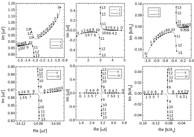
FIG. 1: Saddle points as a function of energy for a Keldysh parameter ofγ = 0.975and scattering angleθ= 0. The first, second and third column give the start time, the return time, and the intermediate drift momentum, respectively. The panels present the paths in the complex plane that are followed by the saddle points as a function of the final energy, which is indicated by the numbers, which are in multiples ofUP.
The upper row gives the saddle points for the pair of orbits with the shortest two travel times(1 + 2), the lower row for(9 + 10), which is one of the pairs with the longest times considered in this paper. The figure shows how the saddle points of a pair approach each other most closely near the classical cutoff. In each case, the contribution of the orbit that is drawn dashed is dropped after the cutoff.
With expansion (25) inserted into the original integral (24), the amplitudeMi+jreduces to a sum of Bessel functions,
Mi+j =
p
2π∆S/3 exp(iS¯+iπ/4) ׯ
A[J1/3(∆S) +J−1/3(∆S)]
+ ∆A[J2/3(∆S)−J−2/3(∆S)] ,
∆S = (Si−Sj)/2, S¯= (Si+Sj)/2, ∆A = (Ai−iAj)/2, A¯= (iAi−Aj)/2,
(26)
where the four independent parameters S¯, ∆S = 2ε3/2(27a)−1/2,A¯=g
0(−2πi)1/2a1/4(3ε)−1/4, and∆A=
g1(2πi)1/2ε1/4(3a)−3/4 have been expressed by the
ampli-tudes and actions that result from the saddle-point approxima-tion of the diffracapproxima-tion integral (24).
The uniform approximation is defined by inserting into Eq. (26) the actions and amplitudes (18) of the respective pair of quantum orbits (which we denoted byi andj). We wish to stress that it is not necessary to obtain the expansion param-etersS¯,ε,a,g0, andg1by explicitly carrying out the
expan-sion (25). Indeed, knowledge of the explicit dependence on these parameters is not even desired because it can be
ma-nipulated by a coordinate transformation, while the original integral is invariant under smooth changes of the coordinate system. For the saddle-point approximation (18), invariance with respect to coordinate transformations is ensured trivially for the actionsSs, while the amplitudesAsare invariant be-cause the Jacobian of a transformation contributes a factor to gwhich is cancelled by the determinant of second derivatives of the action, see Eqs. (18c) and (21b). This is the reason why we express the expansion coefficients in Eq. (25) by the coordinate-transformation invariant quantitiesAi,j,Si,jof the saddle points. Indeed, it is a simple exercise to verify with the help of the asymptotic behavior
J±ν(z)∼
2
πz
1/2
cos(z∓νπ/2−π/4) (27)
of the Bessel functions for largez that the saddle-point ap-proximation (18) is recovered from the uniform approxima-tion (26) in the limit of large∆S.
functions, depending on the integration contour taken in their integral representation. The functional branches can be dis-tinguished by the number of saddles which are visited by a steepest-descent deformation of the contour, in complete anal-ogy with the procedure for the original integral (6). Hence, when the condition (15) is fulfilled one not only observes a Stokes transition in the original integral, but also encounters a Stokes transition in the defining integral of the Bessel func-tions. The proper branch of the function will automatically be selected by requiring a smooth functional behavior. The choice of branches beyond the Stokes transition corresponds to replacing the BesselJ functions by BesselKfunctions,
Mi+j =
p
2i∆S/πexp(iS¯) ׯ
AK1/3(−i∆S) +i∆AK2/3(−i∆S)
.(28)
From the usual asymptotics
Kν(z)∼
π
2z
1/2
exp(−z) (29)
of the BesselK function for largezone verifies that in this case only saddleicontributes to the saddle-point approxima-tion.
In summary, in the uniform approximation the sum of saddle-point amplitudes (18) of each pair of quantum orbits is simply replaced by the collective amplitude (26). The uni-form approximation improves the saddle-point approximation such that it works even when two quantum orbits approach each other so closely that one cannot locally expand about ei-ther one, as is the case close to their classical cutoff. It also works well far away from classical cutoffs, because it includes the saddle-point approximation as a special case which is re-covered for |∆S| >∼ 1. This can happen in two ways: (i) when the saddle points become well separated as a system pa-rameter (such asp) is varied, or (ii) in the strict semiclassical limit when for fixed system parameter the Keldysh parameter is decreased (given∆S 6= 0). Also, the Stokes transition at the classical cutoff is automatically built into the uniform ap-proximation. Most notably, the uniform approximation is of the same practical simplicity as the saddle-point approxima-tion since it involves the same amplitudesAsand actionsSs defined in Eqs. (18).
V. COMPARING THE VARIOUS APPROXIMATIONS
In this section, for the zero-range potential we compare the approximations discussed in the previous sections with the ex-act integration of Eq. (6). First, let us consider ATI spectra in the direction of the electric field of the laser. Such a spectrum is composed of the contributions of direct and of rescattered electrons. The former quickly decrease after their classical cutoff at 2UP. The latter form an extended plateau with its classical cutoff at10UP, whose yield is below that of the di-rect electrons by several orders of magnitude. The cutoff at 10UP is related to the pair of orbits with the shortest travel times. The other pairs of trajectories, which have longer travel times, have cutoff energies below this value (see, e.g., Ref. [6]
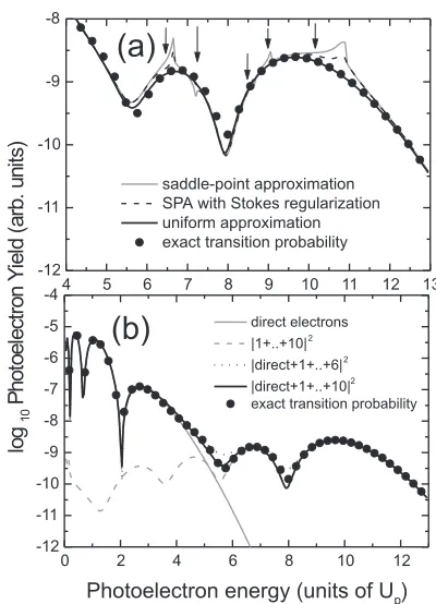
FIG. 2: Photoelectron spectra for a zero-range binding potential and
UP/ω = 3.58, ω = 0.073 a.u.,and a ground-state energy of
E0 = −0.5 a.u.The spectrum is in the direction of the electric field of the laser,θ = 0.Part (a) shows spectra computed using the saddle-point and uniform approximations, compared with the pho-toelectron yield obtained by computing the integral (6) exactly. We take into account the two direct trajectories and five pairs of rescat-tered trajectories. The approximate energy positions of the Stokes transitions, which coincide with the respective classical cutoffs, are indicated by arrows. Part (b) displays spectra computed by means of the uniform approximation, for direct, rescattered, and both types of electrons, and compares these with the exact integration.
for a more complete discussion). In the figures that follow, we consider up to 5 pairs of electron trajectories, those with the shortest travel times. To each trajectory, we associate a pos-itive integer number which increases with the corresponding travel time.
The outcome of this comparison is displayed in Fig. 2(a). In general, there is a good qualitative agreement between the saddle-point approximation and the exact solution (note, how-ever, that the scale is logarithmic in this figure.) Quantita-tively, however, there are marked discrepancies, which occur in those energy regions where the saddle points that consti-tute a particular pair approach each other and can no longer be treated as independent.
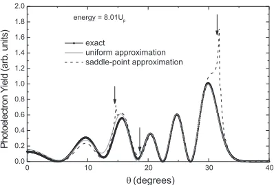
FIG. 3: Angular distributions of photoelectrons for the zero-range potential case, computed with the saddle-point and uniform approx-imations, compared to the exact yield. The field parameters are UP/ω= 35.8,ω= 0.0584 a.u., the ground-state energy is chosen
asE0 =−0.9 a.u., and the photoelectron energy isǫ = 8.01UP. The angles of Stokes transitions are marked with arrows.
is particularly critical if the intensity of the driving field is not so high. In this case, the various cutoff energies are relatively close to each other, so that the artifacts affect a broad energy region. Thus, a more accurate approximation is desirable and even necessary, in case the integral (6) cannot be carried out exactly, as is the case for any potential other than the zero-range potential.
One possibility to eliminate such effects, shown in Fig. 2(a), is the Stokes regularization, Eq. (22). This smoothes out the cusps, without, however, eliminating them completely.
Far superior results are obtained by the uniform approxi-mation, given by Eqs. (26) and (28), respectively. The spec-trum computed in this way almost perfectly agrees with the exact result. The remaining differences between the uniform approximation and the exact integration occur near the inter-ference minima and are due to the contributions of pairs of tra-jectories with longer travel times that have not been included. This is indicated by the minor differences in the spectra com-puted with the uniform approximation using 3 and 5 pairs of trajectories, cf. Fig. 2(b).
Figure 2(b) shows that the exact spectrum is well repro-duced by the uniform approximation for all energies. The figure also separately displays the contribution of the direct electrons [30]. One observes that interference between the rescattered and direct electron trajectories is only important within a small energy region, between 4UP and6UP [31]. Above and below this energy range, either the rescattered or the direct electrons completely dominate the spectrum, so that interference only leads to minor effects.
The superiority of the uniform approximation over the saddle-point approximation becomes particularly impressive if spectra are displayed on a linear scale. This is done in Fig. 3 for an angular distribution at fixed energy. Both with the saddle-point approximation and the uniform approxima-tion, the 10 shortest trajectories are considered. The uniform approximation, again, yields excellent agreement with the ex-act result. Minor differences, for small scattering angles, are
caused by the trajectories with still longer travel times that have not been included. Those do not contribute for larger an-gles. The saddle-point approximation, on the other hand, ex-hibits large discrepancies with the exact results near the clas-sical cutoffs. For the chosen photoelectron energy of8.01UP, there are only three relevant cutoffs, corresponding to the pairs of trajectories 1+2, 5+6, and 9+10. The remaining pairs of tra-jectories do not contribute, since their cutoffs are significantly below8.01UP.
VI. INFLUENCE OF THE POTENTIAL ON RESCATTERING PROCESSES
The preceding section has shown that the uniform approx-imation is a very dependable method, yielding results very close to those obtained from the exact integration. The lat-ter, however, is only feasible for a binding potential of zero range. Therefore, we will rely on the uniform approximation to investigate how the form of the binding potential affects the photoelectron spectrum. The transition amplitude (2) was derived in the context of one electron bound by the potential V(r). In order to simulate a many-electron atom, it can be reasonable to use in the transition amplitude (2) different po-tentialsV(r)for the electron when it tunnels out and when it rescatters [10]. In Refs. [10, 23], the effect of the rescattering potential on the general shape of the high-order spectrum and the ratio of direct over rescattered electrons were investigated as a function of the applied field, for the pair of the two short-est orbits. In particular, the dependence on the atomic species was modeled by a Thomas-Fermi potential. Here, for various model potentials, making use of the additional power afforded by the uniform approximation, we will concentrate on the de-tailed shape of the angular-resolved energy spectrum and on the contributions of the orbits with longer travel times.
Throughout, we shall use the results for the zero-range po-tential
V(r) = p2π
2|E0|
δ(r) ∂
∂rr (30)
as a benchmark. Its form factors (10) and (11) are constants,
Vpk=
1 (2π)2p
2|E0|
(31)
and
Vk0=−
(2|E0|)1/4
2π . (32)
A. Influence of the Coulomb tail
time-dependent Schr¨odinger equation (TDSE) [32], so that we can compare the strong-field approximation with an exact so-lution.
The form factors of the Yukawa potential V(r) = −Zexp(−αr)/rare
Vpk=− Z 2π2
1
(p−k)2+α2 (33)
and
Vk0 = −
√ 2 π
Z5/2
(Z+α)2+ [k+A(t′)]2
= − √
2 π
Z5/2
(Z+α)2−2|E 0|,
(34)
where the saddle-point equation (12) has been used in the last line. Hence, in the saddle-point approximation,Vk0 acts as
a constant; indeed, this is the case for any spherically sym-metric potential. This constant determines the total ionization rate, but has no effect on the shape of the spectrum. Another consequence is that the spectrum of the direct electrons, de-scribed by the amplitude (5), is independent of the form of the binding potential because it only depends onVk0, in contrast
to the spectrum of the rescattered electrons.
The Coulomb form factors can be retrieved from Eqs. (33) and (34) in the limitα→0. Since in this caseE0=−Z2/2,
this leads to the well-known divergence of the Coulomb form factor (34) [4]. This has no effect on the shape of the spec-trum, and the absolute scale can be reestablished, too [33].
In Fig. 4, we compare ATI spectra for the zero-range, the Yukawa, and the Coulomb potential. In view of the Coulomb divergence ofVk0we used the zero-range form factor (32) for
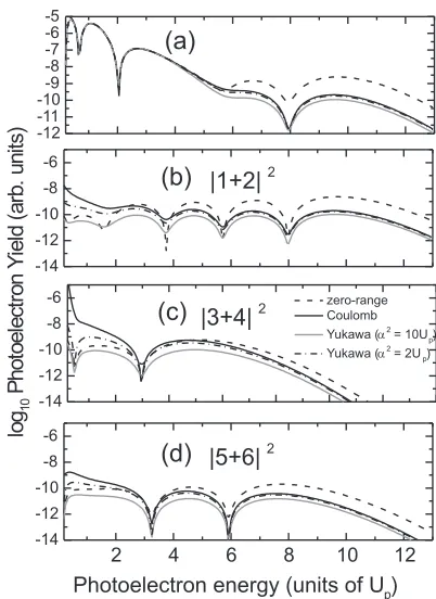
all potentials [34]. As expected from Eq. (33), there is a sup-pression of the photoelectron yield for the higher energies in the Coulomb and Yukawa cases. This effect is present for all pairs of trajectories. For the Coulomb potential, there is an additional enhancement of the rescattered yield for low ener-gies, which does not occur in the zero-range or short-range cases. This enhancement is due to the functional form ofVpk. Clearly, if the screening parameter is small enough, this ef-fect is also present for the Yukawa potential. Furthermore, for these latter potentials, there is a reduction in the plateau in-tensity as the screening parameter is increased. Evidently, the form factor (33) for the Coulomb potential always exceeds the one for the Yukawa potential.
The parameters of Figs. 2 and 4 correspond to those cho-sen in Ref. [32], where the results of a numerical solution of the three-dimensional time-dependent Schr¨odinger equa-tion for hydrogen are reported and ATI spectra are extracted from the former. The agreement between the Coulomb result of Fig. 2 (a) and Fig. 2 of Ref. [32] is good and even quantita-tive. We notice that the pronounced dip in the spectrum near 8UP, which is due to destructive interference of the contribu-tions of the shortest two orbits [cf. Fig. 4 (b)], is almost at the same position in both calculations. The next destructive-interference minimum from these two orbits occurs just below 6UP. The contributions of the longer orbits [cf. Fig. 4 (c) and
FIG. 4: Photoelectron spectra for the zero-range potential, compared with those for the Coulomb and Yukawa potential, for the same field and atomic parameters as in Fig. 2. Panel (a) shows total spectra, while panels (b) to (d) exhibit the contributions of individual pairs of rescattered orbits.
(d)] partially fill in this minimum, leaving only a shoulder in the total spectrum (a). The exact calculation [32] features a slightly more pronounced minimum at the same position. Re-markably, the two interference minima in the total spectrum at low energy near0.5UP and2UP, which are due to the di-rect electrons and the amplitude (5), are also clearly reflected in the exact calculation [32] at about the same positions. The overall drop of the spectrum from the direct electrons to the final maximum of the rescattered electrons preceding the cut-off is more pronounced in the exact calculation by about half an order of magnitude [35].
In Fig. 5, we investigate the ATI spectra for several screen-ing parametersαof the Yukawa potential. In this figure, we also address the question of how the form factorVk0 affects
the photoelectron yield. The figure clearly shows a global shift in the photoelectron signal, which increases for decreas-ingα. In this sense, our results are in agreement with those in Ref. [22]. It is, however, not expected that this yield increases indefinitely. In fact, its limit forα→0should be given by the TDSE results [32]. Because of the singularity for hydrogen inVk0for vanishing screening parameters, such a comparison
FIG. 5: Photoelectron spectra for the Yukawa potential, the same field and atomic parameters as in the previous figure, and several screening parameters α. Part (a) shows the resulting spectra for the direct electrons and the five shortest pairs of rescattered orbits, whereas part (b) shows the contributions from the shortest pair of rescattered trajectories.
B. Shell potentials
Spherical shell potentials have been used for modeling clus-ters or molecules such as C60. Recently, ATI has been
ob-served experimentally for C60in the direct-electron energy
re-gion [36]. Therefore, in this section we investigate how such potentials affect the ATI spectra in the direct and rescattered regions. Let us first consider a sphericalδ-shell,
V(r) =−V0δ(r−r0), (35)
with
V0=
p
2|E0|
1−exp[−2p
2|E0|r0]
, (36)
where E0 again denotes the binding energy of the ground
state. Ionization from such a potential was investigated in the past [37], for weaker laser fields. The corresponding form factors (10) and (11) are
Vpk=−
V0r0
2π2p
(p−k)2sin[
p
(p−k)2r
0] (37)
FIG. 6: Photoelectron spectra for the shell potential (35), compared with the zero-range case. The ionization potential was taken as
|E0| = 0.274a.u. and the cluster radius asr0 = 6.7a.u. The field parameters areI0 = 6.5×10
13
W/cm2
, andω= 0.057a.u. This yields an excursion amplitude ofa0 = 13.2a.u. and a Keldysh parameterγ= 0.9805. In part (a) we take into account the five short-est pairs of trajectories, whereas in part (b) only the shortshort-est pair is considered.
and
Vk0=− V0C
πp
|E0|r0
sinh(p2|E0|r0), (38)
respectively, with
C=
" p
2|E0|
exp(2p
2|E0|r0)−1−2p2|E0|r0
#1/2
. (39)
For theδ-shell potential,Vpk is an oscillating function, and Vk0 is a constant as always. Thus, in the following, we
con-centrate on the influence ofVpkon the resulting spectra. We consider typical C60 parameters, taken from Ref. [36]. The
external field is chosen such that its intensity is still below the C60 fragmentation threshold, but the electron excursion
am-plitude [38] is roughly twice as large asr0. Furthermore, the
Keldysh parameter is about unity. Thus, the rescattering pic-ture is still expected to be applicable.
The figure shows that theδ-shell potential rescatters more ef-ficiently than the zero-range potential by about one order of magnitude. If the form factor (38) is taken into account, an additional global increase in the yield occurs. However, in theδ-shell case, the rescattering plateau on the average has a downward slope, in contrast to the zero-range case where the slope goes up.
The most interesting feature, however, is that the rescattered spectrum of theδ-shell potential is much more structured than it is for the zero-range potential, with several additional oscil-lations. Such oscillations are due to the form factor (37), and are already present for the contributions of the shortest pair of trajectories, as shown in Fig. 6(b). An unexpected side effect of these oscillations is the effective increase of the plateau cut-off energy by about two units ofUP for the shell versus the zero-range potential, which can be observed in Fig. 6. Since the laser intensity is the same in both cases, the rescattering cutoff would be expected at the same energy, too. However, the shell form factor has a zero around the energy of9.5UP, where the zero-range spectrum features its final maximum. This moves the final maximum of the shell-potential spectrum up to a higher energy.
In order to investigate these oscillations in more detail, in the following we will look at contributions of individual tra-jectories to the photoelectron yield for theδ-shell, in compari-son to the zero-range potential. Since the uniform approxima-tion requires pairs of trajectories, we will use the saddle-point approximation for that purpose. Whenever dealing with a pair of trajectories, we will consider the uniform approximation.
Figure 7 displays these results, for several rescattered tra-jectories. In caseVpkis constant, as is the case for the zero-range potential, all oscillations present in the spectra come from interference terms. The contributions of individual tra-jectories are nearly constant in the classically allowed regime and do not produce any substructure. For theδ-shell, however, Vpkis oscillatory and produces its own maxima and minima in the spectrum. However, comparing Fig. 6(a) and (b) we observe that the contributions of the longer orbits tend to re-store the minima of the shell-potential spectrum to those of the zero-range. Only the highest-energy minimum near9.5UP is left unaffected, since the longer orbits do not contribute to this energy.
In particular, the minima are given by Rep(p−k)2 =
nπ/r0, wherenis an integer. To a first approximation, the
drift momentumkcan be neglected with respect to the mo-mentump, so that the energy positions of the minima, in units of the ponderomotive energy, are roughly given by
p2
2UP = n
2π2
r2 0UP
. (40)
This expression is expected to work better for longer excur-sion times, since, according to Eq. (14),k∝1/(t−t′
). This can already be seen in Fig. 1, where the saddle points as func-tions of the energy are depicted. For a pair of trajectories with short travel times, the start and the return times, as well as the intermediate momentum k, vary considerably with the pho-toelectron energy. For a long travel time, on the other hand, these quantities are nearly constant, in the classically allowed
FIG. 7: Contribution from individual trajectories to the rescattered photoelectron spectrum for the shell potential, in comparison to the zero-range case. We consider the same parameters as in the previous figure. The labelsiandjrefer, in part (a), to the third-shortest pair, denoted by (5+6), and in part (b) to the eighth-shortest pair, denoted by (15+16). For the terms|i+j|2
we applied the uniform approxi-mation. For the terms|i|2
+|j|2
, we applied the Stokes regularization (22) to the diverging trajectory. The dashed vertical lines in the fig-ure separate the classically allowed and forbidden energy regions for the respective orbits. The dotted and dashed gray lines in part (a) denote the individual contributions of 5 and 6, respectively, for the zero-range case.
region. Furthermore, the return time, as well as the intermedi-ate momentum, are almost real andkis very small.
Clearly, there exist deviations from Eq. (40) due to the fact thatkis non-vanishing and complex,tandt′
are complex, and due to the time dependence of the intermediate momentum. For instance, a feature that is not explained by Eq. (40) is a shift in the oscillations of the longer trajectory, with respect to those of the short one. This feature occurs for all pairs of trajectories, and decreases as the travel times get longer. A qualitative estimate of these deviations can be obtained by consideringp(p−k)2up to first order in√k2, and the pair
(t1, t′1) and(t2, t′2) = (t1−ε, t′1+ε ′
)up to first order in ε, ε′.This gives a shift in the minima, which is proportional to
ε/(t−t′
),confirming the results presented in Fig. 7.
Now we turn to other shell potentials. Similar results are obtained for a more realistic square well, of the formV(r) = −V0forr1< r < r2, and zero otherwise. Since, in nature, the
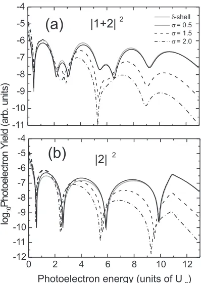
oscil-FIG. 8: Contribution from the shortest pair of trajectories to the photoelectron spectrum for the Gaussian potential (41), compared to the δ-shell case, for several widths σand the same parameters as in the previous figure. Parts (a) and (b) depict |1 + 2|2
and|2|2 , respectively. The prefactorV0, for|E0|= 0.274, was computed by solving the time-independent Schr¨odinger equation numerically.
lations are also present for smooth potentials that approximate Eq. (35). One such example is the Gaussian potential
V(r) =−V0exp[−(r−r0)2/σ2]. (41)
For vanishing width, we recover Eq. (35). For this potential, the form factorVpkis given by a rather complicated expres-sion, which will not be reproduced here. Important features of Vpkare the presence of minima and a decrease with increasing asymptotic momentum. This decrease dampens the oscilla-tions, such thatVpk, in comparison to theδ-shell form factor, decays much more rapidly for largep. This effect becomes more pronounced as the width of the potential increases.
In Fig. 8(a), the contribution of the two shortest trajecto-ries to the ATI spectra is displayed for the Gaussian potential (41), in comparison to theδ-shell potential. We considered the zero-range-potential form factor Vk0 [Eq. (32)]. As in
the previous figure, there exist additional oscillations, which come fromVpk. In Fig. 8(b), this is clearly shown, for the contributions from the second shortest trajectory. For small width, as expected, theδ-shell oscillation pattern is practically recovered. For the parameter range considered in the figure, this holds forσ <∼0.5. Major differences are present only for σ >1.5. As the width gets larger, there is a displacement in the minima of the form factor and a suppression of the
pho-toelectron yield. This suppression is due to the decay of the form factorVpk. Therefore, even when the shell potentials are smoothed out, the oscillations survive. Thus, the possibil-ity that they are artificially caused by the sharp edges of the δ-shell potential can be ruled out.
VII. CONCLUSIONS
We investigate the influence of the binding potential in above-threshold ionization (ATI) for linearly polarized laser fields, in terms of quantum orbits, using the uniform approx-imation [Eqs. (26) and (28)]. In this method, the transition amplitude is expanded in terms of the collective contribution of pairs of orbits rather than individual orbits. No information is required beyond the conventional saddle-point approxima-tion. This is made possible and, indeed, necessitated by the fact that for laser-induced rescattering phenomena the orbits naturally come in pairs that nearly coalesce at the classical cutoffs, thus rendering the conventional saddle-point approxi-mation inapplicable in this energy region. Moreover, the uni-form approximation remains valid beyond the classical cutoff in the classically forbidden region, where it automatically in-corporates the fading out of unphysical saddles beyond the cutoff energy. If the two saddles of a pair are sufficiently far apart, the standard saddle-point approximation is recovered.
The fact that the uniform approximation is valid in the whole energy range, both away from as well as near the cut-offs, allows one to obtain quantitative predictions for ATI spectra. Indeed, in this paper this approximation has been tested for the zero-range potential against the numerical com-putation of the SFA transition amplitudes. The photoelec-tron spectra, as well as the angular distributions obtained in both ways turned out to be practically identical. With the conventional saddle-point approximation, quantitative predic-tions are not possible in certain energy regions, which for low laser intensity can span the better part of the ATI plateau.
The excellent quality of the uniform approximation for the zero-range potential also suggests that the uniform approxi-mation is reliable enough for computing ATI spectra for other binding potentials, such as Coulomb, Yukawa, or shell po-tentials. Within the framework of this paper, the influence of the binding potential is contained in two form factors, which either characterize the transition from the ground state to an intermediate momentum state, or the transition from the inter-mediate state to an asymptotic momentum state. Throughout the paper, these form factors are calledVk0andVpk, respec-tively.
numeri-cal solution of the time-dependent Schr¨odinger equation [32]. Furthermore, for the Yukawa potentials, we observed an in-crease in the yield for decreasing screening parameter. Similar features have been obtained in [22], from the numerical solu-tion of the strong-field approximasolu-tion transisolu-tion amplitudes.
Another class of potentials that we investigated are shell potentials, which are commonly used as an approximation for clusters. In comparison to the zero-range case, the photoelec-tron spectra computed for such potentials exhibit additional structure, which comes from the oscillating form ofVpk. This is an extreme case of how the form factorVpkinfluences the photoelectron yield. Such oscillations are also present when the potentials are smoothed out, and therefore are not an arti-fact of the shell models.
An alternative for performing such investigations is the nu-merical solution of the three-dimensional Schr¨odinger equa-tion. This would require considerable numerical effort, and, for elliptical polarization, it would take one close to the limit of today’s computational resources. Another possibility would be the numerical solution of the strong-field approxi-mation amplitudes (1) and (2). From the numerical viewpoint, this is not an easy task either, since one must deal with mul-tiple integrals of highly oscillating functions. Thus, the uni-form approximation considerably simplifies the computations involved. Furthermore, using this approximation, one is able to gain additional physical insight into the interference
pro-cesses between the quantum orbits, and how such propro-cesses are affected by the binding potential.
Summarizing, the uniform approximation is a very pow-erful method for investigating laser-assisted rescattering pro-cesses, being applicable in all energy regions of the spec-tra. This approximation allows one to compute photoelec-tron spectra for binding potentials other than the zero-range with minimal numerical effort. Application of the methods developed in this paper to other high-intensity laser-induced or laser-assisted phenomena, such as non-sequential double ionization, or to elliptically polarized fields is, in principle, straightforward.
Acknowledgments
This work was supported in part by the Deutsche Forschungsgemeinschaft. We are grateful to S. P. Goreslavskii and S. V. Popruzhenko for useful discussions, to S. V. Popruzhenko for the critical reading of the manuscript, to M. E. Madjet for providing references on clusters, to R. Kopold for giving us his code for computing the exact results, and to A. N. Salgueiro for her collaboration in the early stage of this project.
[1] N. B. Delone and V. P. Krainov, Multiphoton Processes in
Atoms, (Springer, Berlin, 1994).
[2] P. B. Corkum, Phys. Rev. Lett. 71, 1994 (1993).
[3] L. F. DiMauro and P. Agostini, Adv. At., Mol., Opt. Phys. 35, 79 ( 1995).
[4] M. Lewenstein, Ph. Balcou, M. Yu. Ivanov, A. L’Huillier, and P. B. Corkum, Phys. Rev. A 49, 2117 (1994).
[5] M. Lewenstein, K. C. Kulander, K. J. Schafer, and P. Bucks-baum, Phys. Rev. A 51, 1495 (1995).
[6] R. Kopold, W. Becker, and M. Kleber, Opt. Commun. 179, 39 (2000).
[7] P. Sali`eres, B. Carr´e, L. Le D´eroff, F. Grasbon, G. G. Paulus, H. Walther, R. Kopold, W. Becker, D. B. Miloˇsevi´c, A. Sanpera, and M. Lewenstein, Science 292, 902 (2001).
[8] K. C. Kulander, K. J. Schafer, and J. L. Krause, in Super-Intense
Laser-Atom Physics, Vol. 316 of NATO Advanced Study
In-stitute, Series B: Physics, B. Piraux, A. L’Huillier, and K. Rza¸˙zewski (editors), (Plenum, New York, 1991), p. 95. [9] S. P. Goreslavskii and S. V. Popruzhenko, J. Phys. B 32, L531
(1999); Laser Phys. 10, 583 (2000).
[10] S. P. Goreslavskii and S. V. Popruzhenko, Zh. ´Eksp. Teor. Fiz.
117, 895 (2000) [JETP 90, 778 (2000)];
[11] N. Bleistein and R. A. Handelsman, Asymptotic Expansions of
Integrals (Dover, New York, 1986).
[12] M. V. Berry, Proc. R. Soc. Lond. A 422, 7 (1989). [13] H. Schomerus and M. Sieber, J. Phys. A 30, 4537 (1997). [14] I. J. Berson, J. Phys. B 8, 3078 (1975); N. L. Manakov and L.
P. Rapoport, Zh. ´Eksp. Teor. Fiz. 69, 842 (1975) [Sov. Phys. JETP 42, 430 (1976)]; F. H. M. Faisal, P. Filipowicz, and K. Rza¸˙zewski, Phys. Rev. A 41, 6176 (1990); W. Becker, S. Long, and J. K. McIver, Phys. Rev. A 42, 4416 (1990); P. S. Krsti´c, D.
B. Miloˇsevi´c, and R. K. Janev, Phys. Rev. 44, 3089 (1991); G. F. Gribakin and M. Yu. Kuchiev, Phys. Rev. A 55, 3760 (1997). [15] B. Borca, M. V. Frolov, N. L. Manakov, and A. F. Starace, Phys.
Rev. Lett. 88, 193001 (2002).
[16] For a recent measurement of the photodetachment spectrum in H−, see R. Reichle. H. Helm, and I. Yu. Kyan, Phys. Rev. Lett.
87, 243001 (2001).
[17] For a recent review, see W. Becker, F. Grasbon, R. Kopold, D. B. Miloˇsevi´c, G. G. Paulus, and H. Walther, Adv. At., Mol., Opt. Phys., to be published.
[18] P. Hansch, M. A. Walker, and L. D. Van Woerkom, Phys. Rev. A 55, R2535 (1997); M. P. Hertlein, P. H. Bucksbaum, and H. G. Muller, J. Phys. B 30, L197 (1997); H. G. Muller and F. C. Kooiman, Phys. Rev. Lett. 81, 1207 (1998); H. G. Muller, Phys. Rev. Lett. 83, 3158 (1999); M. J. Nandor, M. A. Walker, L. D. Van Woerkom, and H. G. Muller, Phys. Rev. 60, R1771; E. Cormier, D. Garzella, P. Breger, P. Agostini, P. Ch´eriaux, and C. Leblanc, J. Phys. B 34, L9 (2001).
[19] G. G. Paulus, F. Grasbon, H. Walther, R. Kopold, and W. Becker, Phys. Rev. A 64, 021401(R) (2001); C. Figueira de Morisson Faria, R. Kopold, W. Becker, and J. M. Rost, Phys. Rev. A 65, 023404 (2002); R. Kopold, W. Becker, M. Kleber, and G. G. Paulus, J. Phys. B 35, 217 (2002).
[20] L. V. Keldysh, Zh. ´Eksp. Teor. Fiz. 47, 1945 (1964) [Sov. Phys. JETP 20, 1307 (1965)]; F. H. M. Faisal, J. Phys. B 6, L89 (1993); H. R. Reiss, Phys. Rev. A 22, 1786 (1980).
[21] A. Lohr, M. Kleber, R. Kopold, and W. Becker, Phys. Rev. A
55, R4003 (1997).
[22] D. B. Miloˇsevi´c and F. Ehlotzky, Phys. Rev. A 57, 5002 (1998); ibid. 58, 3124 (1998).
477 (1998); Pis’ma Zh. ´Eksp. Teor. Fiz. 68, 858 (1998) [JETP Lett. 68, 902 (1998)].
[24] R. Kopold and W. Becker, J. Phys. B 32, L419 (1999). [25] In practice, the tunneling picture is still applicable ifγ <∼1. [26] In the case of just one variable, as is the case in the direct
am-plitude (1), all these statements can be illustrated in straightfor-ward graphical fashion; for an example, see R. Kopold, doctoral dissertation (Technische Universit¨at M¨unchen, 2001).
[27] G. G. Paulus, W. Becker, and H. Walther, Phys. Rev. A 52, 4043 (1995).
[28] Both imaginary parts are positive: As a rule, any saddle that has a negative imaginary part of the action cannot be visited by the steepest-descent contour. This is so because in the original integration the action was real(ImS = 0), and the deformation procedure does not lead to an increase ofImS, by construction. [29] T. Poston and I. N. Stewart, Catastrophe Theory and its
Appli-cations (Pitman, London, 1978).
[30] Even though the amplitude (2) contains both rescattered and di-rect electrons, in the context of the saddle-point and the uniform approximation it is preferable to calculate the direct electrons from the amplitude (1) and then, to avoid double counting their contribution, to disregard very short quantum orbits(τ≪T)in the amplitude (2); cf. R. Kopold and W. Becker, in Multiphoton
Processes, AIP Conference Proceedings No. 525, (American
Institute of Physics, Melville, NY, 2000), p. 11.
[31] For elliptical polarization, the energy range where direct and rescattered electrons interfere is larger, owing to the faster drop of the rescattered electrons for increasing energy. Indeed, inter-ference between direct and rescattered electrons has been ob-served in this case both in the experiment and in theory; see G. G. Paulus, F. Grasbon, A. Dreischuh, H. Walther, R. Kopold, and W. Becker, Phys. Rev. Lett. 84, 3791 (2000).
[32] E. Cormier and P. Lambropoulos, J. Phys. B 30, 77 (1997). [33] T. Brabec and F. Krausz, Rev. Mod. Phys. 72, 545 (2000). [34] Note that, in addition, for the same parameters as in [32], the
matrix element (34) is singular, such that a direct comparison would not be possible.
[35] Note that our results include the phase-space factor; that is, all of our spectra plot the quantity|p| |M|2.
[36] E. E. B. Campbell, K. Hansen, K. Hoffmann, G. Korn, M. Tchaplyguine, and M. Wittmann, Phys. Rev. Lett. 84, 2128 (2000).
[37] G. P. Arrighini, C. Guidotti, and N. Durante, Phys. Rev. A 35, 1528 (1987); S. Patil, Phys. Rev. A 46, 3855 (1992).