82 | P a g e
STUDY OF FISHEYE ROUTING PROTOCOL IN NS3
AND ITS COMPARATIVE ANALYSIS WITH AODV,
DSDV & OLSR
1
Anindya Sankar Roy,
2Mayuri Borah,
3Arpita Banerjee
1
Engineer, Department of Research and Development, Toshniwal Enterprises Controls Limited, (India) 2
Engineer, Department of Research and Development, Toshniwal Enterprises Controls Limited, (India) 3
Associate Prof. Department of Electronics and Communication Engineering, RCCIIT, Kolkata, (India)
ABSTRACT
In this paper, we present a novel routing protocol for wireless ad hoc networks – Fisheye State Routing (FSR) in
NS3. FSR introduces the notion of multi-level fisheye scope to reduce routing update overhead in large networks.
Nodes exchange link state entries with their neighbors with a frequency which depends on distance to destination.
From link state entries, nodes construct the topology map of the entire network and compute optimal routes.The
second part of the thesis is about comparing the other established Ad hoc routing protocols like AODV , DSDV ,
OLSR with FISHEYE in random waypoint model with high mobility , high traffic and speed . We have tested that
over a small network of 20 nodes finding out packet delivery ratio , delay and other factors and have tried to find
out the best solution for 20 nodes environment.
Key words:AODV, DSDV, DSR, Fisheye, NS3
I INTRODUCTION
83 | P a g e
Fig1: Simple MANET example
Wireless networking is an emerging technology that will allow users to access information and services electronically, regardless of their geographic position. The use of wireless communication between mobile users has become increasingly popular due to recent performance advancements in computer and wireless technologies. This has led to lower prices and higher data rates, which are the two main reasons why mobile computing is expected to see increasingly widespread use and applications.
There are two distinct approaches for enabling wireless communications between mobile hosts. The first approach is to use a fixed network infrastructure that provides wireless access points. In this network, a mobile host communicates to the network through an access point within its communication radius. When it goes out of range of one access point, it connects with a new access point within its range and starts communicating through it. An example of this type of network is the cellular network infrastructure. A major problem of this approach is handoff, which tries to handle the situation when a connection should be smoothly handed over from one access point to another access point without noticeable delay or packet loss Another issue is that networks based on a fixed infrastructure are limited to places where there exists such network infrastructure.
84 | P a g e A key feature that sets ad-hoc wireless networks apart from the more traditional cellular radio systems is the ability to operate without a fixed wired communications infrastructure and can therefore be deployed in places with no infrastructure. This is useful in disaster recovery, military situations, and places with non-existing or damaged communication infrastructure where rapid deployment of a communication network is needed.
A fundamental assumption in ad-hoc networks is that any node can be used to forward packets between arbitrary sources and destinations. Some sort of routing protocol is needed to make the routing decisions. A wireless ad-hoc environment introduces many problems such as mobility and limited bandwidth which makes routing difficult.
This thesis researches existing traditional routing protocols, examines current proposed mobile ad-hoc routing protocols, and then designs and implements a functional link-state routing protocol employing a novel “fish-eye” updating mechanism specific for a wireless infrastructure. This mechanism is then analyzed to evaluate its effectiveness and the advantages it can offer.
II FISHEYE ROUTING PROTOCOL 2.1 Protocol Overview
In this work our main focus is on the Fisheye Routing Protocol. The goal is to provide an accurate routing solution while the control overhead is kept low. The proposed scheme is named “Fisheye Routing” due to the novel „fisheye‟ updating mechanism. Similar to Link State Routing, Fisheye Routing generates accurate routing decisions by taking advantage of the global network information. However, this information is disseminated in a method to reduce overhead control traffic caused by traditional flooding. Instead, it exchanges information about closer nodes more frequently than it does about farther nodes. So, each node gets accurate information about neighbors and the detail and accuracy of information decreases as the distance from the node increases.
85 | P a g e
2.2 Algorithm
There are 3 main tasks in the routing protocol:
1) Neighbor Discovery: responsible for establishing and maintaining neighborrelationships.
2) Information Dissemination: responsible for disseminating Link State Packets(LSP),which contain neighbor link information, to other nodes in the network.
3) Route Computation: responsible for computing routes to each destination using theinformation of the LSPs.
Each node initially starts with an empty neighbor list and an empty topology table. After its local variables are initialized, it invokes the Neighbor Discovery mechanism to acquire neighbors and maintain current neighbor relationships. LSPs in the network are distributed using the Information Dissemination mechanism. Each node has a database consisting of the collection of LSPs originated by each node in the network. From this database, the node uses the Route Computation mechanism to yield a routing table for the protocol. This process is periodically repeated.
In [14], Kleinroch and Stevens proposed the fisheye technique to reduce the size of information required to represent graphical data. The original idea of fisheye was to maintain high resolution information within a range of a certain point of interest and lower resolution further away from the point of interest. For routing, this fisheye approach can be interpreted as maintaining a highly accurate network information about the immediate neighborhood of a node and becomes progressively less detailed as it moves away from the node.
86 | P a g e
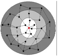
Fig 2: Application of fisheye in a network.
The reduction of routing messages is achieved by updating the network information for nearby nodes at a higher frequency and remote nodes at a lower frequency. As a result, considerable amount of LSPs are suppressed. When a node receives a LSP, it calculates a time to wait before sending out the LSP from the following equation:
UpdateInterval = ConstantTime * hopcount^alpha
ConstantTime is the user defined default refresh period to send out LSPs(in the first scope), hopcount is the number of hops the LSP has traversed, alpha is a parameter that determines how much effect each scope has on the Update Interval. Values for alpha are zero(same as no fisheye) and greater than or equal to one(fisheye). A maximum value of Update Interval is established to prevent an effective complete suppression of LSP messages(when calculated UpdateInterval is too large).
When a router accepts a LSP from a faraway node, and has not yet sent out the LSP in memory, the next time it will send out the LSP will be the minimum of the time left to wait in memory and the new calculated UpdateInterval based on the new LSP:
UpdateInterval(new) = MIN(UpdateInterval(memory), UpdateInterval(LSP))
This is to prevent a router from waiting indefinitely to send out a LSP when a new LSP arrives before the one in memory is sent out for that node.
2.3 Route Computation
87 | P a g e 1) Link State Database- Contains the LSPs the node received.
2) PATH- contains ID, path cost, forwarding direction tuples. Holds the best path found. 3) TENT- contains ID, path cost, forwarding direction tuples. Holds possible best paths. The Djikstra algorithm is as follows:
1) Start with “self” as the root of a tree by putting (myID, 0, 0) in PATH.
2) For node N just place in PATH, examine N‟s LSP. For each of N‟s neighbors, add the total path cost at N to the cost path of each neighbor. If the new total path of the node is better than the value for that node in PATH or TENT, put into TENT.
3) If TENT is empty, terminate the algorithm. Otherwise, find the minimal cost in TENT, move into PATH, and go to Step 2.
One the algorithm completes, PATH now contains the shortest next-hop information for each destination. The protocol can now use the PATH database as a routing table to forward packets toward their destinations.
III IMPLEMENTATION 3.1 Software used
Network Simulator 3 (NS3): ns-3 is a discrete-event network simulator for Internet systems, targeted primarily for research and educational use. ns-3 is free software, licensed under the GNU GPLv2 license, and is publicly available for research, development, and use.
The goal of the ns-3 project is to develop a preferred, open simulation environment for networking research: it should be aligned with the simulation needs of modern networking research and should encourage community contribution, peer review, and validation of the software.
88 | P a g e Fig 3: Modules in NS3
3.2 Creating a Client server architecture for routing of packets
The first step to start implementing routing protocols in mobile environment starts with packet transfer between two nodes i.e a client and a server architecture. It shows the three way handshake that takes place in the process of packet transfer from the server to the client.
Fig 4: NS3 Running Window
Header file used -
1. point-to-point-module.h, is the main header file used in this basic scenario
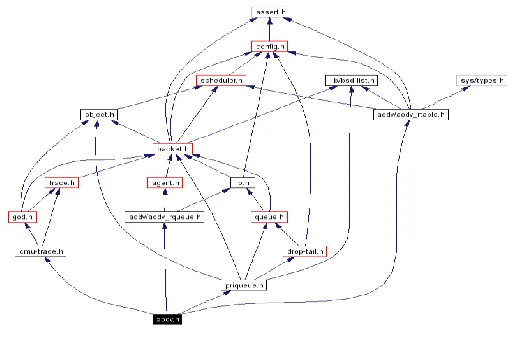
3.3 Implementing AODV in a small network scenario a) File Dependency of AODV Protocol
89 | P a g e example is been described
Fig 5: File Reference of ‘AODV.CC’
The header files responsible for running the AODV are :- aodv-module.h, core-module.h, network-module.h , internet-network-module.h , mobility-network-module.h, point-to-point-network-module.h, wifi-network-module.h, v4ping-helper.h
90 | P a g e
b) Implementing Fisheye in NS3
The Fisheye routing protocol was simulated in a mobile environment to determine the connectivity among mobile hosts. The simulator for evaluating the protocol is Network Simulator 3 environment. NS3 provides a discrete-event simulation environment for wireless network systems.
IV SIMULATION ENVIRONMET
In the simulation process the environment taken has 20 nodes. All nodes are mobile in nature and follows the random waypoint model to define the movement nature of the nodes. The speed assigned to the nodes is 20 m/s, the wifi module is used to simulate the ad-hoc wireless environment.
4.1 Modules used :point to point module , network module, application module, wifi module, mobility module, csma module , internet module, netanim module, flow monitor module, gnuplot, aodv module, dsdv module, olsr module, Fisheye module
4.2 Mobility models in NS3:Constant Position, Constant Velocity, Constant Acceleration, Gauss Markov, Hierarchical, Random Direction2D, Random Walk2D, Random Waypoint, Steady State Random Waypoint
4.3 TheRandom – Waypoint model: It is used in this scenario as what we have seen is that, this model best depicts the real life scenario in which all the nodes are mobile. Some stop at an arbitrary time for arbitrary time and then again continues to move at an arbitrary direction.
AODV Simulation results in NS3 for 20 nodes.
91 | P a g e
Fig 9: Packet Delivery ratio curve for 20 nodes Fig 10: Packet Loss curve for 20 nodes DSDV Simulation results in NS3 for 20 nodes.
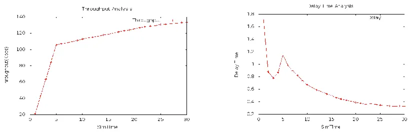
Fig 11: DSDV Throughput curve for 20 nodes Fig 12: DSDV Delay Time curve for 20 nodes
92 | P a g e
OLSR Simulation results in NS3 for 20 nodes.
Fig 15: OLSR Throughput curve for 20 nodes Fig 16: OLSR Delay curve for 20 nodes
Fig 17: OLSR Packet Delivery Ratio curve for 20 nodes Fig 18: OLSR Packet Loss curve for 20 nodes
Fisheye Routing Protocol Simulation results in NS3 for 20 nodes.
93 | P a g e
Fig 21: Fisheye PDR curve for 20 nodes Fig 22: Fisheye Packet Loss curve for 20 nodes. V CONCLUSION
The Fisheye Routing Protocol module is built on NS3 as the first phase of Thesis work. The table of comparative study of the four routing protocols including the Fisheye Routing Protocol is done using NS3 simulation is shown above, the graphs received are shown above the table. The table shows that the Fisheye Routing protocol functions good in a small environment of 20 nodes .In case of OLSR the curve for 20 nodes is very unstable and the value shows steep fall to 0. DSDV has better performance than OLSR but not as Fisheye Routing protocol .But the Delay characteristics is best in case of Fisheye, as it shows very less delay for 20 nodes scenario . So from this analysis we can conclude that Fisheye Routing Protocol has best performance for 20 nodes scenario. The future continuation of the work is to implement all four protocols in large environment which is 100 nodes scenario and comparative analysis of both the result.
REFERENCES
[1] F. Maan, N. Mazhar; “MANET Routing Protocols vs Mobility Models: A Performance Analysis” in ICUFN 2011
[2] A. Tuteja, R. Gujral, S. Thalia; “Comparative Performance Analysis of DSDV, AODV and DSR Routing Protocols in MANET using NS2”, in 2010 International Conference on Advances in Computer Engineering. [3] A. Rehman, F. Anwar, J. Naeem, S. M. Abedin; “A Simulation Based Performance Comparison of Routing
Protocol on Mobile Ad-hoc Network” in International Conference on Computer and Communication Engineering (ICCCE 2010) Kuala Lumpur, Malaysia.
94 | P a g e
International Journal of Advancements in Computing Technology, Volume 3, Number 1 February 2011.
[5] C. Lal, V. Laxmi, M. S. Gaur; “Performance Analysis of Manet Routing Protocols for Multimedia Traffic.” In
International Conference on Computer & Communication Technology (ICCCT)-2011
[6] M. Kassim, R. A. Rahman, R. Mustapha; “Mobile Ad-hoc Network (MANET) Routing Protocols Comparision
for Wireless Sensor Network”
[7] G. Fang, L. Yuan, Z. Qingshun, L. Chunli; “Simulation and Analysis for the Performance of the Mobile Ad-hoc
Network Routing Protocols” in The Eight Internation Conference on Electronic Measurement and Instruments. [8] Farhat Anwar, Md. Saiful Azad, Md. ArfaturRahman, MdMosheeud din; “Performance Analysis of Ad hoc
Routing Protocols in Mobile WiMax Environment” IAENG International Journal of Computer Science, Vol 35, issue 3, September 2008.
[9] GeethaJayakumar and G. Gopinath; “Performance Comparison of two on demand routing protocol for Ad-hoc
Networks based on random way point mobility Model”. American Journal of Computer Science and Network Security(IJCSNS 2007), vol VII, no 11 pp. 77-84, November 2007.
[10]Y. Chaba, Y. Singh, M. Joon; “Simulation based Performance Analysis of On-Demand Routing Protocols in
MANETs” in 2010 Second International Conference on Computer Modeling and Simulation.
[11] M. Morshed, F.I. S. Ko, D. Lim, H. Rahman, R. Rahman, J. Ghosh; “Performance Evaluation of DSDV and
AODV Routing Protocols in Mobile Ad-hoc Networks.”
[12]Nadia Qasim, Fatin Said, Hamid Aghvami; “ Mobile Ad Hoc Networks Simulation Using Routing Protocols for
Performance Comparisions”, Proceedings of world Congress on Engineering 2008 vol 1 WCE 2008, July 2-4,2008 London, U.K.
[13]Charles E.Perkins and Elizabeth M_Royer,“Ad hoc on demand distance vector (AODV) routing (Internet-Draft)”,Aug-1998.
[14]L. Kleinrock and K. Stevens, "Fisheye: A Lenslike Computer Display Transformation," Computer Science Department, UCLA, CA Tech. Report,1971