Adaptive Multilevel Splitting for Monte Carlo particle transport
Henri Louvin1,, Eric Dumonteil2, Tony Lelièvre3, Mathias Rousset3, and Cheikh M. Diop1
1CEA Saclay, DEN/DM2S/SERMA/LTSD, F-91191 Gif-sur-Yvette 2IRSN, PSN-EXP/SNC, F-92262 Fontenay-aux-Roses
3Université Paris-Est, CERMICS (ENPC), INRIA, F-77455 Marne-la-Vallée
Abstract. In the Monte Carlo simulation of particle transport, and especially for shielding applications, vari-ance reduction techniques are widely used to help simulate realisations of rare events and reduce the relative errors on the estimated scores for a given computation time. Adaptive Multilevel Splitting is one of these variance reduction techniques that has recently appeared in the literature. In the present paper, we propose an alternative version of the AMS algortihm, adapted for the first time to the field of particle tranport. Within this context, it can be used to build an unbiased estimator of any quantity associated with particle tracks, such as flux, reaction rates or even non-Boltzmann tallies. Furthermore, the efficiency of the AMS algorithm is shown not to be very sensitive to variations of its input parameters, which makes it capable of significant variance reduction without requiring extended user effort.
1 Introduction
The challenge in using Monte Carlo particle transport simulations for shielding applications is to minimize the computation time required to attain a reasonable variance on the quantity of interest, calledscore.
The basic approach of variance reduction techniques is to modify the simulation behaviour so as to increase rare events occurrence while keeping an unbiased estimator of the score.
In this view,multilevel splitting techniqueswere intro-duced to the field of particle transport by Kahn and Harris [1]. The principle of these techniques is to increase the number of simulated particles when approaching areas of interest of the geometry. Practically, the simulated space is divided into regions of importance, and the particles that pass from a less important to a more important region are duplicated. Each of the duplicated particles is given half the weight of the original to ensure that the simulation remains unbiased. Thus, more computation time is spent to simulate interesting particles rather than new particles from the source.
The downside of these techniques is that they require a fair knowledge of the system in order to accurately define the importance regions. More recently, a new method called Adaptive Multilevel Splitting (or AMS) has been proposed by Cérou and Guyader [2], and studied in a more general setting by Bréhier et al. [3]. This method also aims to duplicate the interesting particles of the simulation, but uses the knowledge accumulated during the simulation itself to determin on the fly which particle
should be duplicated and at which point. One of the
e-mail: [email protected]
most interesting feature of AMS is that it requires little knowledge of the system to yield interesting results. The efficiency of the AMS in Monte Carlo simulations and its properties makes it attractive for computational physics problems that require precise rare event simulation. To this end, AMS was successfully extended to molecular dynamics simulations by Aristoffet al. for the resampling of reactive paths [4].
In this paper, we aim to apply the AMS algorithm to Monte Carlo particle transport, and demonstrate its efficiency for rare event simulations. In Section 2, we will describe a mathematical version of the AMS algorithm specifically designed to fit the requirements of particle transport. We introduce in Section 3.1 the context of the study, which is neutral particle transport with the Monte Carlo method. The core of this work is presented in Section 4, in which we introduce for the first time a pratical implementation of AMS within a Monte Carlo particle transport simulation. This version of the AMS algorithm was implemented in the development version of the Monte Carlo particle transport code TRIPOLI-4R. In the last Section of this paper, we present some of the results obtained using AMS within TRIPOLI-4R. These examples illustrate the validity of the algorithm as described in Section 4, as well as the efficiency of AMS as a variance reduction technique.
2 Mathematical setting
of the AMS is a variant of the algorithm which perfectly fits the theoretical frame from [3], so that the estimator of the rare event occurence probability introduced in the following is unbiased.
2.1 Objective and setup
LetX=(Xt)t∈Nbe a discrete-time Markov chain with
val-ues inRd,d ∈ N∗. We define Pas the path space, con-taining all possible realisations of the Markov chain X. Given T a subset of Rd, we define the entrance time of the Markov chainXinT:
τT =inf{t∈[0;τf] :Xt∈T},
whereτf is the final stopping time of the Markov chainX,
which we suppose finite.
Given an observableφT :P →Rsuch asφT =0 on the
eventτf < τT, we would like to estimate the averageφT
ofφT. Let us suppose now that the probability for (Xt) to
enterT beforeτf is very small, i.e. P(τT < τf) 1. In
such a case of rare event simulation, the AMS algorithm proposes to reduce the variance on the estimated average by increasing the number of Markov chains reaching the subset T. AMS is an iterative algorithm that consists of several steps. The first step is a basic Monte Carlo sim-ulation of multiple replicas of the Markov chain X with a common initial state. Each of the following steps con-sists in the resampling of some Markov chains amongst the replicas, with an initial condition getting closer toT at each iteration of the algorithm.
2.2 AMS algorithm
2.2.1 Importance function
We define a so-calledimportance function, mappingRdto
R:
ξ:Rd→R,
which is used to quantify the proximity of a point inRdto
the subset of interestT. The only requirement imposed on ξis that there exists a constantZT ∈Rsuch that
ξ(x)≥ZT if x∈T
ξ(x)<ZT if xT. (1)
We further define the importanceof a Markov chain
X=(Xt)t∈Nas the supremum ofξalong the chain:
Ξ(X)=sup
t∈N
ξ(Xt). (2)
The ξfunction is probably the most important ingre-dient of the AMS algorithm, since it is used to quantify the proximity of a path to the subset T. It is therefore important to choose a good functionξwith regards to the rare event we are trying to simulate. Even if the AMS algorithm is proven to yield an unbiased resultregardless of ξ, the choice of an optimized importance function is
expected to improve the variance reduction efficiency. We will discuss further the issue of the quality of the function ξin Sect. 5.
2.2.2 Initialization
The AMS algorithm consists in an interacting system of weighted replicas. Givenn>0, we simulateni.i.d. repli-cas of the Markov chain X, denoted by X0j = (X0j,t)t∈N,
j∈ {1, . . . ,n}. For all j, the initial stateX0j,0 is a pointx0
located outside ofT. We defineZ0as
Z0=ξ(x0).
Let us denote by q ∈ N the current iteration num-ber, and by k the number of replicas resampled at each iteration.Within an iteration of the AMS algorithm, every replica hasthe same weight. The global weight at iteration
qwill be denotedWq, withW0set to 1.
For the sake of simplicity, we present in the following the case where distinct paths cannot have the same impor-tance. The general case is discussed in Section 2.3. Now we can start iterating onq≥0.
2.2.3 Iterations
(i) For each j ∈ {1, . . . ,n}, denote byτqj,f the stopping time of the Markov chainXqj, and bySqj its
impor-tance (See (2):
Sqj = Ξ(Xqj). (3)
(ii) Sort the sample (S1
q, . . . ,Snq) in increasing order:
S(1)q < . . . <S(k)q < . . . <S(n)q .
(iii) Denote byZq+1thek-th order statisticsSq(k):
Zq+1:=S(k)q .
(iv) IfZq+1 ≥ZT, stop iterating and go to the final step
(See Sect. 2.2.5)
(v) For allj∈ {1, . . . ,k}, resample replicaX(qj)according
to the resampling kernel described in Sect. 2.2.4, and denote it byXqj+1
(vi) For all j∈ {k+1. . . ,n}, defineXqj+1 =X(qj)
(vii) Update the global weight:
Wq+1=
n−k n Wq
(viii) Incrementqand go to step (i)
2.2.4 Resampling process
At each iteration of the AMS algorithm,kreplicas are sampled. These Markov chains undergo the following re-sampling procedure:
Let us denote the current iteration number byqand the associated resampling level byZq+1.
For each of thekreplicasX(j),j∈ {1, . . . ,k}to be
re-sampled, one of the remaining replica X(i),i > kis
Markov chain (X(i)t )t∈[0;τ(i)
f] contains at least a state whose
importance is greater thanZq+1 (otherwise it would have
been resampled). We can therefore define
τ(i) q =inf
t∈[0;τ(i)q,f] :ξ(Xq(i),t)>Zq+1
as the first time at which the replicaX(i)has an importance
greater thanZq+1.
The resampled Markov chain (Yt)t≥0 is defined as a
replica of the Markov chainXwith initial condition
Y0=X(i)q,τ(i) q
.
2.2.5 Final step
Once the algorithm stops iterating, we denote by N the number of completed iterations. Given the bounded ob-servableφT introduced in Sect. 2.1, we define
ˆ φT =
n
j=1
WNjφT(XNj) (4)
as anunbiasedestimator of the averageφT[3].
2.3 Interpretation of the replicas weights
In this section we provide a practical interpretation of the AMS weights to give an intuition on the estimator (4). The mathematical proofs of the unbiasedness and consistency of the AMS estimator are not presented in this paper. We refer the reader to [2] and [3] for theoretical support.
At each iteration q ≥ 0, the level Zq+1 is chosen in
such a way that the probability for a pathXqj to have an
importance greater thanZq+1(i.e. P(Sqj ≥Zq+1|Sqj ≥Zq))
is estimated by
ˆ
pq=1−
k n.
Keeping that in mind, we can see that the weights of the replicas at iteration q+1 are nothing more than an estimate of the probabilityP(Sqj+1≥Zq+1).
In other words, the AMS algorithm provides us at each iterationqwith a set of pathsXqj, j∈ {1, . . . ,n}, carrying a
global weight, which can be interpreted as an estimate of the probability to have this particular set of paths instead of the paths sampled at iteration 0.
2.4 About the number of resampled replicas
The algorithm presented in Sect. 2.2 is an ideal case. In reality, it may occur that multiple replicas have the same importance. In that case, the number of replicas having an importance less or equal to thek-th lowest importance may very well be greater thank. When such a situation arises,everypath which importance is less or equal to the level has to be resampled.
This modification has to be taken into account in the repli-cas weights. If the current iteration is theq-th and the num-ber of particles to be resampled isK>k, then the weight update at step (vii) of the algorithm has to be changed to:
Wq+1=
n−K n Wq.
In some pathological configurations, all the replicas may happen to have the same importance, which would lead to extinction at the next iteration. In that case, the iterating process is interrupted and the algorithm goes straight to the final step (See Sect. 2.2.5), eventually yielding a null contribution.
3 Monte Carlo neutral particle transport
3.1 Neutron transport theory
The transport theory describes the mathematical frame-work needed to solve the equations governing the behavior of a gaz of non-interacting particles (e.g. neutrons, pho-tons) in different materials, under different assumptions (spins are not taken into account, relativistic effects are neglected etc.). It has been discussed at length in [6] or [7]. In fissile materials, neutrons (and photons) can induce fissions, which results in the production of more particles. The modelling of such systems is achieved using the so-called critical linear Boltzmann equation. When the mate-rials are not fissile, the standard linear Boltzmann equation can be used to describe the particle transport.
It is assumed that the neutral particles in homoge-neous medium are transported along straight lines between collisions points and are randomly reoriented at each in-teraction (with eventual change of energy) [8]. As the flights lengths are exponentially ditributed, the underlying stochastic process governing the neutral particle transport is calledexponential flights. We refer the interested reader to [9, 10] for recent developments on this topic.
3.2 Monte Carlo simulation of neutral particle transport
Numerically, transport problems are stochastically solved
using Monte Carlo transport codes [11]. Those codes
simulate directly the particles trajectories according to laws of probability provided by the so-called nuclear data (cross sections, energetic and angular transfers, secondary particles emission spectrums, etc.), which are available in international libraries. The flights lengths between interactions are randomly sampled, as well as the outgoing direction and energy of the particle after each collision with the medium.
Every Monte Carlo transport code relies on the particle tracking routine, which simulates the random life of the particles by transporting them from one interaction to another, until they are absorbed or leak out of the geometry.
Within a Monte Carlo simulation, the life of each transported particle is build step by step, which means that the state of the particle at a given time is determined exclusively from the knowledge of its state after the
previous interaction. This makes the random process
algorithm described in Section 2 can be implemented.
4 Neutral particle transport with AMS
The goal of this section is to present a practical implemen-tation of the AMS algorithm in the context of Monte Carlo particle transport.
4.1 Definitions and notations
Before going any further, let us introduce some definitions and notations which will be used throughout the follow-ing.
We define the position of a particle in the
6-dimensional phase space S as the set of coordinates
(X,Ω,E), where X denotes the particle position in the 3-dimensional space,Ωits direction, andEits energy.
A particle is considered alive while it is transported from an interaction to the next. When an interaction results in the capture of the particle, the transport stops and the particle is referred to askilled. We calltrackof a particle the sequence of its interaction points.
We call geometrythe subspace of the phase space in which the simulation takes place. If a particle is trans-ported to a point of the phase space that is not included in the geometry, this particle is considered leaking out of the geometry and is instantly killed.
The aim of the simulation is to estimate a score
(typically a flux or a reaction rate) in a particular volume of the geometry we will refer to as detector or simply
target.
4.2 Importance map
As we saw in Sect. 2.2.1, the geometry has to be provided with an importance function, so as to determine the regions of the system that are of interest to the simulation. Tech-nically, we will use a function that associates any point of the phase space to an importance value, which is related to the probability for a particle located at this point to con-tribute to the final score. We will refer to this function as
importance functionorimportance map, and denote it by
I(X,Ω,E).
In order to satisfy the requirement (1), it is sufficient to define an importanceItargetlarger than any other value
on the map, and to assign it to every point of the target volume. In TRIPOLI-4R, Itarget is set to the numerical equivalent of positive infinity regardless of the importance values outside the target volume, so as to avoid mistakes.
4.3 The AMS algorithm
As described previously, the AMS algorithm is an iterative method. Each iteration includes the definition of a single splitting level alongside with the corresponding splitting process.
4.3.1 Initialization (stepq=0)
Let nbe the initial number of simulated particles, andk
theuser-definednumber of particles that are to be dupli-cated at each iteration of the algorithm. The initial par-ticles are simulated using an analog Monte Carlo simula-tion (i.e.without variance reduction), and the track of each transported particle is kept in memory.
There are actually many ways to store a particle track. For the AMS algorithm to be the most performant, this track should only contain the emission point of the par-ticle and the coordinates of the parpar-ticle after each intera-cion with the geometry. The coordinates of a particle at an interaction point but before the interaction takes place should not be stored, as the importance function relate to the probability for a particle simulated from a given point of the phase space to contribute to the score, and that prob-ability usually takes into account the fact that the particle is transported before interacting with the medium.
The global weight at iterationqis denoted bywq, and
w0is set to 1. We can now start iterating onq≥0.
4.3.2 Iterations (q≥0)
Each trackT is given an importance value, defined as the maximum importance of the points of its track:
I(T)= max
i∈trackI(Xi,Ωi,Ei). (5)
Thentracks are sorted according to their importance, and the k-th smallest track importance defines the splitting levelIq+1.
If Iq+1 is greater than Itarget, the iterating process
stops. Otherwise, all the tracks that have an importance less or equal to the level Iq+1 are suppressed, and the
same number of tracks are randomly selected (with replacement) amongst the remaining tracks. The selected tracks are duplicated at their first collision point of importance greater thanIq+1, according to the resampling
kernel presented in Sect. 2.2.4. The global weight is then updated:
wq+1=
n−Kq
n wq
= q
i=0
(1−Ki
n ),
whereKqis the number of resampled particle tracks at
it-erationq(See Sect. 2.3).
4.3.3 Final step and scoring
As soon as a splitting levelIqis greater thanItarget, the
al-gorithm stops iterating. We defineN =q−1. The score ˆ
φtargetin the target is then computed using the standard
es-timators of Monte Carlo particle transport, as for an analog simulation, but using the last set of tracks.
An unbiased estimator of the flux in the target is built by weighting the estimated flux ˆφtargetby the probability
of reaching the last splitting level (See Sect. 2.2.5):
ˆ
4.4 Strengths of the AMS
4.4.1 Number of contributions to the score
In order to reduce the variance when simulating rare events, it is interesting to have multiple small contribu-tions to the score rather than a few large contribucontribu-tions and many zeroes.
The stopping criterion of the AMS algorithm offers a guarantee thatat least n−k+1 particles will reach the target and contribute to the score with a small weightwN,
except for pathological cases. However, the cases of ex-tinction are rare and caused by the use of a very unadapted importance map.
4.4.2 Robustness with regard to the importance function
The estimator constructed as described in Sect. 4.3 is un-biasedregardless of the parameterk[2]. The same holds true for any importance map under the single constraint [3]:
Itarget∈]Isource,+∞[. (6)
In our implementation of the AMS algorithm, this condition is always verified, as we set the importance of the target to infinity regardless of the importance map (see Sect. 4.2). This allows us to use any function as importance. However, if the map does not properly describe the system, the result, though unbiased, will probably take a really long time to converge.
4.4.3 Usability
In addition to the usual parameters of any Monte Carlo particle transport simulation, AMS introduces only two free parameters: the number of duplicated particlesk, and the importance mapI(X,Ω,E).
As we already pointed out, any choice of k and I
yields an unbiased result. The parametrization of the AMS algorithm is therefore quite simple. It is sufficient to define a purely geometric importance function, such as the inverse to the distance to the target, and to set any value forkless thann to reduce the variance. More efficiency can be achieved through the use of a precise importance map, taking into account the direction and energy of the particles.
4.4.4 Parallelization
A Monte Carlo simulation performed with AMS yields a single value as estimation of the quantity of interest. Therefore, multiple independant simulations are required to obtain a precise result. The arithmetic mean of the estimations over all simulations is computed, as it is
the case in regular Monte Carlo. As the simulations
remain totally independant until their output is gathered to compute the average result, a straightforward way of parallelizing AMS Monte Carlo is to run independant simulations on several processors simultaneously.
5 Validation and results
The AMS algorithm was implemented in the develop-ment version of the Monte Carlo particle transport code
TRIPOLI-4R [5]. This 3D continuous-energy Monte
Carlo code is developed by the Service d’Etudes des Réac-teurs et de Mathématiques Appliquées (SERMA) at CEA Saclay.
In the following, we present some preliminary
re-sults obtained with TRIPOLI-4R using AMS and
com-pare them to simulations with no variance reduction. The Monte Carlo simulations that do not use any variance re-duction techniques are usually calledanalog, because they are directly analogous to the natural transport of the parti-cles.
We aim to validate the AMS algorithm implementation and to estimate its efficiency as a variance reduction tech-nique by comparing its results and performances to analog TRIPOLI-4R simulations.
5.1 Figure of merit
In a Monte Carlo simulation, the flux is estimated for several statistical independent groups of particles (or
batches). The average flux and its associated variance are estimated from the series of batches. The purpose of vari-ance reduction is to reduce the varivari-ance of the result for a given computation time. The efficiency of a variance re-duction technique lies upon two factors. On one hand, the relative errorσof the average flux, and on the other hand the simulation timeT. If we denote byNBthe total number
of simulated batches, we have
σ∼ √1
NB
and T ∼NB. (7)
We use the figure of merit (FOM) to evaluate the effi -ciency of a Monte Carlo simulation. The FOM is defined as
FOM= 1
σ2T, (8)
and should remain relatively constant during the simula-tion according to (7). For different simulations of the same system, the simulation producing the largest FOM is ei-ther proportionally faster or more precise than the oei-thers. Therefore, the FOM can be used as a performance mea-surement for variance reduction.
5.2 Importance map calculation
The AMS algorithm implemented in TRIPOLI-4R can use several functions as importance maps.
The user can define apurely geometricalimportance, such as the distance between a point and the particle source or the invert of the distance between a point and the AMS target.
TRIPOLI-4R, which is used for other variance reduction techniques in this code and to automatically pre-computes an importance map (see [5]).
5.3 Bypass simulation
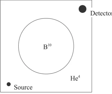
The first system consists of an extruded box filled with Helium. The dimensions of the box are 10cm×10cm×+∞. A neutron flux is produced from an 15-MeV isotropic neutron source at one corner of the box and estimated inside an infinite cylinder of 1cm in diameter placed at the opposite corner. Inbetween is a massive infinite cylinder composed of highly concentrated Bore. The mean free path of neutrons in the Bore slab is less than 0.5 cm. The geometry for this problem is shown in Fig. 1.
Source
Detector
He
4B
10Figure 1.Bypass simulation configuration
The results obtained using TRIPOLI-4R without
vari-ance reduction and TRIPOLI-4R using the AMS
algo-rithm are presented in Table 1. Several AMS simula-tions with 104initial particles were performed, with diff
er-ent values for the parameterk, from 1 duplicated particle (0.01%) per iteration up to 5×10³(50%). In all
simula-tions, theINIPONDimportance map was used.
We observe that the AMS significantly improves the FOM regardless of the parameter k. The number of it-erations required for the AMS algorithm to complete in-creases withkup to kn =0.5%. Above this value, the com-putation time per simulation remains stable and the FOM gain relatively constant.
The smallest relative error for a given number of in-dependent simulations is obtained with k = 1 (0.01%). However, this configuration requires a very large number of iterations for the AMS to complete, which has a strong impact on the computation time. It is therefore more in-teresting (regarding the FOM gain) to chose a greaterkin order to speed up the simulation.
The study of the Bypass problem puts into light the ap-parent robustness of the AMS efficiency with regard to the parameterk. As long as it is not too small, its impact on the algorithm efficiency in reducing the variance remains stable. However, it is to be noted that the geometry of the Bypass configuration is fairly simple. We may find
cases in which the number of splitting per iteration have a greater impact on the algorithm efficiency.
5.4 Neutron flux attenuation in water
The source of the second problem is a directional neutron point source, emitting neutrons according to a Watt spec-trum and placed at the entry of a straight box filled with water. The detector is placed at 3 m from the source, and the neutron flux is estimated in 10-cm-thick slices between the source and the detector.
3m
1m
Source
Detector
Figure 2.Water box simulation system
The neutron flux attenuation was estimated using
both analog and AMS TRIPOLI-4R simulations. In a
first realization, the importance function used for the AMS was the distance from the source point. The AMS was performed using 103 initial particles per batch and
k = 102 splitting per iteration. Data were collected for both simulations during 65h. Fig. 3 presents the estimated flux with respect to the distance in the box, and the
associated 99.7% confidence intervals. The FOM for
these simulations are shown in Fig. 4.
Depth (cm)
50 100 150 200 250 300
Neutron flux
18 −
10
16 −
10
14 −
10
12 −
10
10 −
10
8 −
10
6 −
10
4 −
10
2 −
10 1
2
10
Analog
AMS (geometrical) Analog
AMS (geometrical)
Table 1.Comparison of TRIPOLI-4R with and without AMS for flux estimation in the Bypass geometry (48h calculations)
Simulation Number of independent simulations Mean Relative error FOM Gain
Analog 14300 4.3042×10⁻¹⁰ 8.6838×10⁻² 0.0008 1
AMS (0.01%) 210 4.0541×10⁻¹⁰ 1.5377×10⁻² 0.0246 31
AMS (0.05%) 1705 4.2244×10⁻¹⁰ 7.1384×10⁻³ 0.1135 147
AMS (0.1%) 4038 4.1462×10⁻¹⁰ 3.8072×10⁻³ 0.3992 517
AMS (0.5%) 10170 4.1518×10⁻¹⁰ 2.3973×10⁻³ 1.0075 1307
AMS (1%) 10900 4.1547×10⁻¹⁰ 2.3948×10⁻³ 1.0123 1313
AMS (5%) 10884 4.1494×10⁻¹⁰ 2.4280×10⁻³ 0.9816 1273
AMS (10%) 11472 4.1451×10⁻¹⁰ 2.3604×10⁻³ 1.0387 1347
AMS (50%) 10829 4.1591×10⁻¹⁰ 2.3750×10⁻³ 1.0259 1331
Depth (cm)
50 100 150 200 250 300
Figure of Merit
6 −
10
5 −
10
4 −
10
3 −
10
2 −
10
1 −
10 1 10
2
10
3
10
Analog
AMS (geometrical) Analog
AMS (geometrical)
Figure 4.FOM comparison in the Water box
It can be seen in Fig. 3 that the analog simulation in unable to estimate a flux farther than 160cm from the source, because of the strong attenuation of neutrons in water. However, the AMS simulation is able to accurately determine the neutron flux all the way from the source to the detector. Near the source point, the analog simulation
is more efficient than the AMS, as shown in Fig. 4.
The neutron flux in this part of the box is high enough for TRIPOLI-4R not to need variance reduction, which places the AMS at a disadvantage due to its impact on runtime.
The AMS mechanism starts to be interesting at a depth of 70cm. The gain in FOM increases up to 103in favor of
AMS at 160cm, from which point the analog simulation fails to estimate the flux.
In order to illustrate the role of the importance map within the AMS algorithm, the deep-penetration simulation was performed a second time, using the same parameters for AMS except for the geometrical impor-tance function, which was replaced by the imporimpor-tance estimated using theINIPONDmodule. The fluxes obtained with both importance maps are shown in Fig. 5, and the associated FOM in Fig. 6.
We observe that the use of theINIPONDmap over the geometrical importance significantly improves the AMS
Depth (cm)
50 100 150 200 250 300
Neutron flux
18 −
10
16 −
10
14 −
10
12 −
10
10 −
10
8 −
10
6 −
10
4 −
10
2 −
10 1
2
10
AMS (geometrical)
AMS (INIPOND) AMS (geometrical)
AMS (INIPOND)
Figure 5.Flux attenuation in the Water box
Depth (cm)
50 100 150 200 250 300
Figure of Merit
6 −
10
5 −
10
4 −
10
3 −
10
2 −
10
1 −
10 1 10
2
10
3
10
AMS (geometrical)
AMS (INIPOND) AMS (geometrical)
AMS (INIPOND)
Figure 6.FOM comparison in the Water box
5.5 Gamma spectroscopy
The AMS algorithm has the specificity to provide a group of particle tracks associated to a global weight
(see Sect. 4). This feature let us hope to use AMS to reduce the variance on deposited scores, such as deposited spectrum (pulse height tally), energy or charge, for which all particles contributing to the scoremusthave the same weight.
The use of other variance reduction techniques for quantities that depend on collective effect of a group
of particles is a complex problem [12]. Currently,
TRIPOLI-4R does not even support variance reduction with deposited scores. However, AMS offers a possibility to have an efficient variance reduction for deposited scores using the same algorithm than for other types of scores.
We present in Fig. 7 a deposited spectrum obtained by simulating the response of a high-purity Germanium (HPGe) detector placed at 50cm of a Sodium source. The gain in efficiency with AMS is shown in Fig. 8.
Energy (MeV)
0 0.5 1 1.5 2 2.5 3 3.5 4
Deposited spectrum
11 −
10
10 −
10
9 −
10
8 −
10
7 −
10
6 −
10
5 −
10
4 −
10
3 −
10
2 −
10
1 −
10 1
Analog AMS Analog AMS
Figure 7.Deposited spectrum in the HPGe detector
Energy (MeV)
0 0.5 1 1.5 2 2.5 3 3.5 4
Figure of Merit
1 −
10 1 10
2
10
3
10
4
10
5
10
6
10
Analog AMS Analog
AMS
Figure 8.AMS gain in FOM over the deposited spectrum
These results are from photon-only simulations, as the coupled photons/electrons/positrons AMS is not yet fully operational.
6 Conclusion
These preliminary results show that the use of the Adaptive Multilevel Splitting algorithm in TRIPOLI-4R reduces significatively the variance. Its connection to the TRIPOLI-4R importance map calculation module enables us to use advanced parametrizations for the importance. The guarantee to have an unbiased resultregardless of the importance map or the number of particles resampled at each iteration makes the AMS algorithm a viable alternative to existing variance reduction techniques in the most severe configurations. Furthermore, it can also be used for variance reduction on deposited scores without need to alterate the algorithm, as seen in Sect 5.5.
In the future, we plan to implement AMS variance reduction on deposited scores using coupled pho-tons/electrons/positrons simulations as well as coupled neutrons/gamma problems.
Another concern is the comparison of the AMS efficiency to existing variance reduction techniques. A paper by the same authors is in preparation regarding this study [13].
Aknowledgement
TRIPOLI-4R is a registered trademark of CEA. We grate-fully acknowledge EDF for their long term partnership and AREVA for their support.
The work of T. Lelièvre and M. Rousset is supported by the European Research Council under the European Union’s Seventh Framework Programme (FP/2007-2013)
/ERC Grant Agreement number 614492.
References
[1] H. Kahn, T.E. Harris, Nat. Bur. Stand. Appl. Math. Series,Estimation of particle transmission by random sampling,12:27-30 (1951)
[2] F. Cérou, A. Guyader, Stoch. Anal. Appl., Adaptive multilevel splitting for rare event analysis,25(2) :417-443 (2007)
[3] C.-E. Bréhier, M. Gazeau, L. Goudenège, T. Lelièvre, M. Rousset, Ann. App. Prob., Unbiasedness of some generalized Adaptive Multilevel Splitting algorithms(to be published)
[4] F. Cérou, A. Guyader, T. Lelièvre, D. Pommier, J. Chem. Phys.,A multiple replica approach to simulate reactive trajectories,134:054108 (2011)
[5] E. Brun, F. Damian, C.M. Diop, E. Dumonteil, F.X. Hugot, C. Jouanne, Y.K. Lee, F. Malvagi, A. Mazzolo, O. Petit, J.C. Trama, T. Visionneau, A. Zoia, Ann. Nucl. Energ.,TRIPOLI-4R, CEA, EDF and AREVA reference
[6] J. J. Duderstadt, W. R. Martin, Transport theory
(1979)
[7] G. I. Bell, S. Glasstone,Nuclear reactor theory(1970) [8] K. Pearson, Nature,The problem of the random walk,
72:294 (1905)
[9] A. Zoia, E. Dumonteil, A. Mazzolo, S. Mohamed,
J. Phys. A: Math. Theor., Branching exponential
flights: travelled lengths and collision statistics,
45(42):425002 (2012)
[10] A. Zoia, E. Dumonteil, A. Mazzolo, S. Mohamed,
Phys. Rev. E, Collision densities and mean
resi-dence times for d-dimensional exponential flights,
83(4):041137 (2011)
[11] N. Metropolis, S. Ulam, J. Am. Stat. Assoc., The Monte Carlo method,44(247):335-341 (1949)
[12] T. E. Booth, Nucl. Sci. Eng., A Monte Carlo vari-ance reduction approach for non-Boltzmann tallies,
116(2):113-124 (1994)
[13] E. Dumonteil, T. Lelièvre, H. Louvin, M. Rousset,