Efficient SAR Raw Data Simulation Including Trajectory Deviations and Antenna Pointing Errors

Efficient SAR Raw Data Simulation including Trajectory Deviations

and Antenna Pointing Errors

Yuhua Guo1, 2, *, Qinhuo Liu1, Bo Zhong1, and Xiaoyuan Yang3

Abstract—Synthetic aperture radar (SAR) raw signal simulation is profoundly useful for validating SAR system design parameters, testing the effectiveness of different processing algorithms, studying the effects of motion errors, etc. Simulating signal data in frequency domain is more efficient than in time domain. However, the former is difficult account for the effects of both sensor trajectory deviations and antenna pointing error for the stripmap SAR mode. In this paper, we attempt to extend the possibility of the Fourier domain approach to account for trajectory deviations as well as antenna beam pointing errors, which is more concerned for airborne SAR systems. After demonstrating a full two-dimensional Fourier domain simulation, an efficient simulation approach is proposed under certain reasonable assumptions. The proposed approach has higher computational efficiency than simulation in time-domain and also allows for imaging an extended scene. The validity of the proposed approaches is analyzed and discussed. Finally, numerical examples are presented to verify the effectiveness and efficiency of the approach.

1. INTRODUCTION

Synthetic aperture radar is an active microwave remote sensing system that images, with high spatial resolution, an area over the ground. The high resolution in range direction is achieved by transmitting a large bandwidth pulse, whereas the azimuth direction is obtained by using a coherent processing approach to synthesize a long azimuth aperture [1].

SAR raw signal simulation is useful and even indispensable, in sensor design, mission planning, image understanding and interpretation, to name a few [2–15]. For airborne SAR systems, due to the inevitable atmospheric turbulence, platform trajectory and attitude variations are unavoidably induced into sensor parameters. SAR raw signal simulation offers a powerful tool to assess, and subsequently to mitigate, the effect of these motion errors. Time-domain simulation [16–19] is able to exactly account for the effects of motion errors, but for extended scenes, it is computationally inefficient. Frequency-domain simulation, based on the fast Fourier transform (FFT), for the ideal case was presented in [20– 25]. Since the SAR system transform function (STF) depends on the azimuth and range coordinates of the ground targets, the frequency domain approach cannot be directly used to simulate SAR raw signal in the presence of motion errors, some improved methods have been proposed [26–31]. The approach presented in [26] considered a two-dimensional (2-D) Fourier domain simulation that accounts for the effects of sensor trajectory deviations. It has a high processing efficiency by using 2-D Fourier transform, but assuming a narrow-beam-slow-deviation make it only applicable to limited SAR system. Another paper [27] presented a simulation approach that can be applied to lager trajectory deviations than

Received 21 October 2016, Accepted 27 December 2016, Scheduled 12 January 2017

* Corresponding author: Yuhua Guo ([email protected]).

1 _{State Key Laboratory of Remote Sensing Science, Institute of Remote Sensing and Digital Earth, Chinese Academy of Sciences,}

No. 20A, Datun Road, Chaoyang District, Beijing 100101, China. 2 State Key Laboratory of Space-Ground Integrated Information Technology, Beijing Institute of Satellite Information Engineering, No. 5 Minzuyuan Road, Chaoyang, District, Beijing 100029, China.

3 _{Department of Mathematics and Systems Science, Beihang University, No. 37 Xueyuan Road, Haidian District, Beijing 100191,}

the one shown in [26]. However, both of the approaches shown in [26] and [27] only deal with sensor trajectory deviations, not including antenna attitude variations. A Fourier domain simulation approach was presented in [28] for antenna attitude variations. This approach is based on the 2-D Fourier domain formulation of the SAR raw signal including antenna beam pointing errors, but it does not take into account the effects of sensors trajectory deviations. A hybrid-domain approach for the spotlight SAR mode was proposed in [29], which account for low to medium squinted angles including platform motion errors. SAR raw data simulation in the presence of sensor trajectory deviations was given in [30]. This approach is based on a narrow bandwidth approximation and is able to simulate higher aperture angles. Reference [31] proposes a frequency-domain stripmap-mode raw data generator of an extended scene taking the antenna pattern deviation into consideration for fixed and variant squinted geometries.

Generally, platform attitude variations may cause antenna boresight offset in both azimuth and range directions, in which the azimuthal offset is more serious as far as image focusing is concerned. In this paper, we consider both the sensor trajectory deviations and platform attitude variations, which is of more realistic and concerned for airborne SAR systems. As for scattering characteristics, which are dependent on frequency, polarization, and target geometry and dielectric properties, in theory, should be considered as far as quantitative evaluation of radiometric resolution is concerned. Simulation of scattering matrix from complex target is also of interest, which however is beyond the scope of this paper. Readers may be referred to [32] for detailed discussion.

The rest of the paper is organized as follows. The algorithm for trajectory deviations is presented in Section 2. In Section 3, SAR signal simulations are carried out considering the trajectory deviations and antenna attitude variations. Simulation results are discussed in Section 4 to show the effectiveness of the proposed approaches. Finally, conclusions are drawn to close the paper.

2. RAW DATA SIMULATION IN THE PRESENCE OF TRAJECTORY DEVIATION

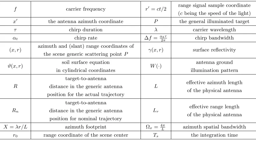
For comparison of the proposed method and corresponding time domain method and also for understanding the following presentation, we firstly summarize the main results obtained in [26] and [27]. Note that h0(x, r) is used to denote the SAR signal in the presence of trajectory deviations. Some important symbols used can be referred to Table 1.

Table 1. List of symbols.

f carrier frequency r=ct/2 range signal sample coordinate

(cbeing the speed of the light)

x _{the antenna azimuth coordinate P the general illuminated target}

τ chirp duration λ carrier wavelength

αt chirp rate Δf=α₂t_πτ chirp bandwidth

(x, r) azimuth and (slant) range coordinates of

the scene generic scattering pointP γ(x, r) surface reflectivity

ϑ(x, r) soil surface equation

in cylindrical coordinates W(·)

antenna ground

illumination pattern

R

target-to-antenna distance in the generic antenna

position for the actual trajectory

L effective azimuth length

of the physical antenna

Rn

target-to-antenna

distance in the generic antenna position for nominal trajectory

Lr effective range length

of the physical antenna

X=λr/L azimuth footprint Ω_x=4_Lπ azimuth spatial bandwidth

2.1. Small Trajectory Deviations

Assume that the transmitted signal is a chirp pulse and the received SAR signal in the presence of trajectory deviations, after the heterodyne step, is:

h0(x, r) = rect

r−R cτ /2

W2

x−x

X dxdrγ(x, r) exp

−j4π λ R−j

4π λ

Δf /f cτ (r

_−R)2

. (1)

From Figure 1, the slant ranges Rn and R take the forms [26]:

Rn =

r2_{+ (x−x)}2 _{=r+ ΔR(x−x, r) (2)} R = (r+δrxr(x, x, r))2+ (x−x)2. (3)

From the geometry shown in Figure 2, the termδrxr(x, x, r) is given by:

δrxr(x, x, r)≈ −d(x) sin(ϑ(x, r)−β(x)) (4)

whered(x) =|d|andβ(x) are related to the horizontal and vertical platform displacements [26]. When displacements are much smaller than the target slant range, the approximation in Eq. (4) is established. Then the slant rangeR can be separated as follows [26, 27]:

R(x, x, r) = Rn(x−x, r) +δR(x, x, r)

= r+ ΔR(x−x, r) +δr(x) +ψ(x, r) +ϕ(x, x, r) (5) where δr(x) is the projection of the trajectory deviations onto the scene center, ψ(x, r) the range variant term, and ϕ(x, x, r) includes the azimuth variant effect. δr(x), ψ(x, r) and ϕ(x, x, r) can be computed using Eq. (4).

As given in [26], a major step in simulation flow is to obtain the following equations, after the range Fourier transform (FT) of the SAR raw data in Equation (1), followed by separating the factor exp{−j(η+4_λπ)δr(x)}from the integral,

h0(x, η) = exp

−j

η+4π

λ

δr(x) ¯h0(x, η). (6)

The next step is to take the azimuth FT of Equation (6), i.e.,

¯

h0(ξ, η) =

exp[−jηr¯ ]

G(ξ−l, η, r) ¯F(ξ−l, l, η, r)dl (7)

Figure 2. SAR system geometry in cross track plane [26].

with

¯

F(χ, l, η, r) =

¯

f(x, x, η, r) exp(−jxχ)·exp(−jxl)dxdx (8)

G(ξ, η, r) = rect

_η

bcτ

w2

ξ

Ω_x

exp

jη 2

4b

exp

−jη¯2_−ξ2_{−η¯r (9)}

¯

f(x, x, η, r) = γ(x, r) exp−jη¯[ψ(x, r) +ϕ(x, x, r)] (10) whereG(·) is SAR STF andη=η+4_λπ.

It shows in [26] that if the following three conditions hold simultaneously:

|ϕ(x, x, r)| λ

4π (11)

|ψ(x, r)| f Δf

λ

2π (12)

|ψ(x, r)−ψ(x, r)| λ

4π (13)

Then a full 2-D Fourier domain approach is attainable. A detailed discussion on the above conditions can be referred to [26].

2.2. Moderate Trajectory Deviations

If conditions in Eqs. (11) and (12) hold, Equation (10) takes the following approximation:

¯

f(x, x, η, r)≈γ(x, r) exp

−j4π λ ψ(x

_{, r) (14)}

The SAR STF,G(·) can be separated into two different contributions as follows:

G(ξ, η, r) =GA(ξ, r)GB(ξ, η, r) (15) where

GA(ξ, r) =ω

ξ

Ω_x

exp

⎡ ⎣_−j

⎛ ⎝4π

λ

2

−ξ2− 4π λ

⎞ ⎠_r

⎤

accounts for the azimuth frequency modulation including the focus depth effect, while

GB(ξ, η, r) = rect

_η bcτ ω ξ Ω_x exp jη 2 4b exp

−jη¯2_−ξ2_−η¯r

exp

⎡ ⎣_j

⎛ ⎝4π

λ

2

−ξ2₋4π λ

⎞ ⎠_r

⎤

⎦ (17)

describes the range cell migration effect.

It follows that Equation (7) can be simplified as:

¯

h0(ξ, η)≈

exp[−jηr¯ ]GB(ξ, η, r){Q(ξ, r)⊗_ξ[GA(ξ, r)Γ(ξ, r)]}dr. (18)

Once ¯h0(ξ, η) is computed, thenh0(x, η) can be evaluated through Eq. (6). It follows thath(x, r) can be readily obtained after range inverse FT.

3. RAW DATA SIMULATION IN THE PRESENCE OF TRAJECTORY DEVIATIONS AND ANTENNA ATTITUDE VARIATIONS

The SAR received signal in the presence of trajectory deviations and azimuth antenna pointing error can be expressed as follows:

h(x, r) =

dxdrγ(x, r) exp

−j4π λR−j

4π λ

Δf /f cτ (r

_−R)2

rect

r−R cτ /2

W2

x−x−δx X

. (19)

Note that the azimuth envelope term, W2(x−_Xx−δx) in Equation (19), is different from that in Equation (1) with the additional term that accounts for antenna pointing error:

δx = (r+δrxr(x, x, r))δaz(x) (20)

δaz(x) is the antenna pointing errors in the azimuth dimension. It can be observed that the antenna

pointing error leads to gain variations, appearing as amplitude modulations. Compared with the case of accounting for antenna attitude variations without trajectory deviations [28], the amplitude modulation in Eq. (20) depends on the actual range coordinate estimation of the target via the term

r+δrxr(x, x, r). Indeed, Equation (19) can be served as a signal model for the exact time-domain

simulation. Theoretically, it is used as a reference to assess the effectiveness of the proposed algorithm, to be presented below.

Since the amplitude modulation depends on both the azimuth position of sensor and the target-to-antenna range, simulation in 2-D Fourier domain is not feasible. Suppose the target-to-antenna pointing errors are small compared with the beamwidth, the following approximation can be taken:

W2

x−x−δx X

≈W2

x−x X

−W2(1)

x−x X

(r+δrxr(x, x, r))δaz(x)

+1 2W

2(2)

x−x X

(r+δrxr(x, x, r))2δ2az(x) (21)

whereW2(n)(·) denotes thenth order derivative of the two-way antenna radiation diagram. Accordingly, the expression of Eq. (19) can be approximated as:

h(x, r)h0(x, r) +h1(x, r) +h2(x, r) (22) where h0(x, r) is the nominal raw data in the presence of trajectory deviations, but free of antenna pointing errors. The latter two terms in the right side of Eq. (22) denote the effect of trajectory

deviations and azimuth antenna pointing error. It should be noted that the difference of the

approximation of the antenna pattern between Equation (21) and that made in [28] is that each component of Eq. (21) is related to the trajectory deviations error. The decomposition of W2(n)_(·)

3.1. Small Trajectory Deviations and Antenna Attitude Variations

For the approach in 2-D Fourier domain, h0(x, r) can be evaluated by the procedures outlined in Section 2.1. For the terms h1(x, r) and h2(x, r), it is highly desirable to evaluate them in a form similar to h0(x, r), such that fast computation in 2-D Fourier domain can be attempted. Note that

h1(·) andh2(·) include both the trajectory deviations and azimuth antenna pointing error, which couple the azimuth and range space-variant effects of the displacement motion error. Hence, it is preferable, even necessary, to decouple the effects of trajectory deviations and azimuth antenna pointing error. In doing so, let us denote the range FT of h1(x, r) as h1(x, η), then it is readily recognized that

h1(x, η) = exp−jηδr¯ (x)h1(x, η). (23)

The term δaz(x) can be taken out from the integral of ¯h1(x, η)

h1(x, η) =δaz(x)h1(x, η) (24) where

h1(x, η) = rect

_η bcτ exp jη 2 4b

dxdrγ(x, r) exp

−jη¯(r+ ΔR(x−x, r)

+ψ(x, r) +ϕ(x, x, r)) −(r+δr(x, x, r))W2(1)

x−x X

(25)

and

b= 4π

λ

Δf /f

cτ . (26)

From Equation (24), it can be seen that the trajectory deviations and antenna pointing errors are now decoupled, to large degree, allowing the azimuth FT of h1(x, η) to be expressed as

h1(ξ, η) = FT[δaz(x)]⊗h1(ξ, η) (27)

whereh1(ξ, η) is the azimuth FT ofh1(x, η) and is given by:

h1(ξ, η) =

drexp[−jηr¯ ]

dlG1 (ξ−l, η, r)F1(ξ−l, l, η, r). (28)

The term F1(·) in the above equation is the 2-D FT of ˜f1(·), where

f1(x, x, η, r) =−[r+δrxr(x, x, r)]γ(x, r) exp−jη¯[ψ(x, r) +ϕ(x, x, r)] (29)

and

˜

G1(x, x, η, r) = rect

_η bcτ PRF v W 2

ξ−Δξ(r) 2Ω_x

−W2

ξ 2Ω_x exp j η 4b ×exp jη 2 4b

exp{−j(η2_−ξ2_−η2_{)r}. (30)}

In Equation (30), note that Δξ(r) = _λr4_PRFπv [28]. It is seen thatf1(·) depends on the trajectory deviations and ˜G1(·) involves the variations of the antenna pattern which is induced by the antenna pointing error effect. Similarly, the 2-D FT ofh2(x, r) can be obtained by the same manner. After the range FT of

h2(x, r), and separating the factor exp{−jηδr(x)}, the azimuth FT of h2(x, η) is

h2(ξ, η) = FT_x[δ2_az(x)]⊗h2(ξ, η) (31)

where

h2(ξ, η) =

drexp[−jηr]

dlG2 (ξ−l, η, r)F2(ξ−l, l, η, r). (32)

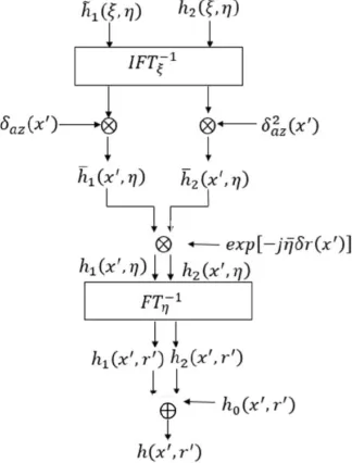
Figure 3. Flow-chart of the SAR raw data simulation.

includes ₂1[r + δrxr(x, x, r)]2. G2 (ξ, η, r) is similar to G1 (ξ, η, r) except that G2 (ξ, η, r) involves

(PRF_v )2[W2(ξ−_ΩΔ_xξ)−2W2(ξ−Δξ(r)_Ωx +W2(ξ−2Δξ(r)_Ωx )] instead of (PRF_v )[W2(ξ−_ΩΔ_xξ) +W2(_Ωξ_x)]. Then, the spectrum of ˜h1(x, r) and ˜h2(x, r) can be obtained. Finally,h(x, r) is evaluated according to the flow chart given in Figure 3.

Recall that ˜f1(·) and ˜f2(·) involve the azimuth and range space-variant effects of the displacement motion error, computation in a full 2-D Fourier domain is not yet feasible at this point. Hence, it is required to take an effective estimation of ˜f1(·) and ˜f2(·). Unlike the approximation made in Section 2.1, now both the amplitude and phase approximations should be put together to evaluate ˜f1(·) and ˜f2(·) as follows:

f1(x, x, η, r) ≈(r+δrr(x, r))γ(x, r) exp{−jηψ¯ (x, r)}=γ1(x, r) (33)

f2(x, x, η, r) ≈ 1

2(r+δrr(x

_{, r))}2

γ(x, r) exp{−jηψ¯ (x, r)}=γ2(x, r). (34)

While the approximation for the phase in ˜f1(·) and ˜f2(·) requiring to meet, simultaneously, the conditions specified in Equations (11), (12) and (13), approximation of ˜f1(·) and ˜f2(·) for the amplitude should satisfy the following condition:

δrxr(x, x, r)≈δrr(x, r) (35)

which is equivalent to (see appendix):

|d(x)|=|d(x)|. (36) That is, the offset of trajectory deviations along the azimuth direction are equal to the trajectory deviations with respect to the target. When conditions in Eqs. (11)–(13) and (35) are all satisfied,

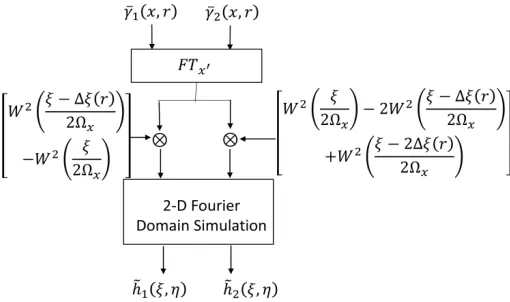
h1(ξ, η) andh2(ξ, η) can be evaluated using the 2-D FT method. The procedure can be illustrated in Figure 4.

The validity limit of the simulator should satisfy Eqs. (11)–(13), (21), (35). From the analysis in Section 2.1, it can be deduced that conditions in Eqs. (11)–(13) lead to the approach only applicable for narrow-beam-slow-deviation. In addition, the condition in Eq. (21) requires that

δx

X 1 (37)

that is

δaz(x) _r+δrX

r(x, r) < X

r = λ

Figure 4. Flow-chart of the method discussed in Section 3.1.

3.2. Moderate Trajectory Deviations and Antenna Attitude Variations

In the previous section, the 2-D FT of SAR raw data simulation accounting for small trajectory deviations and antenna pointing errors is considered. However, the approach requires satisfying the condition of narrow-beam-slow-deviation, making it pertinent to some specific SAR systems. To remove this limitation, one-dimensional azimuth Fourier domain processing followed by range time-domain integration is used. Now that the major task is to evaluate h1(x, r) and h2(x, r). When h1(ξ, η) and

h2(ξ, η) are available, evaluation ofh1(x, r) andh2(x, r) can be performed according to the procedures in Figure 3. Hence, it only requires to evaluate h1(ξ, η) and h2(ξ, η) as described in the following. The difference of the evaluation of h1(ξ, η) and h2(ξ, η) with respect to h0(ξ, η) is that in the evaluation of

f1(·) andf1(·) we have to consider both the amplitude and phase approximation. For the evaluation of

f1(·), let

f1(x, x, η, r)≈(r+δrr(x, r))γ(x, r) exp

−j4π λψ(x

_{, r). (39)}

The conditions of approximation in the above equation with respect to the phase off1(·) are the same as given in Section 2.2, i.e., Eqs. (11) and (12), while the approximation for the amplitude off1(·) should satisfy the following condition:

δrxr(x, x, r)≈δrr(x, r). (40) Then f1(·) can be separated into two terms, which are related to x and x variables. Hence, F1(·) in Eq. (28) can be separated as:

F1(χ, l, η, r) = Γ(χ, r)Q1(l, r) (41) where Γ(·) is the FT of γ(·) [27] and

Q1(l, r) = FT_x

[r+δrr(x, r)] exp

−j4π λ ψ(x

_{, r) . (42)}

Accordingly, G1 (·) in Eq. (30) can be decomposed into the following two parts:

G1(ξ, η, r) =GA(ξ, r)GB1(ξ, η, r) (43)

where

GB1(ξ, η, r) = rect

η

2bcτ /2

PRF

v W

2

ξ−Δξ

2Ω_r

−W2

ξ

2Ω_r

×exp

jη 2

4b exp{−j(

η2_−ξ2−_η2_)r}exp

⎧ ⎨ ⎩j

⎛ ⎝4π

λ

2

−ξ2−4π λ

⎞ ⎠_r

Then h1(ξ, η) can be evaluated as follows:

h1(ξ, η)≈

drexp[−jηr¯ ]GB1(ξ, η, r){Q1(ξ, r)⊗ξ[GA(ξ, r)Γ(ξ, r)]}. (45)

Similarly, after assuming

f2(x, x, η, r) ≈1

2(r+δrr(x

_{, r))}2

γ(x, r) exp

−j4π λψ(x

_{, r) (46)}

the evaluation ofh2(ξ, η) can be obtained by:

h2(ξ, η)≈

drexp[−jηr¯ ]GB2(ξ, η, r){Q2(ξ, r)⊗ξ[GA(ξ, r)Γ(ξ, r)]}. (47)

The difference between Q1(·) and Q2(·) is that Q2(·) includes the term 1₂(r + δrr(x, r))2 instead of (r +δrr(x, r)). Correspondingly, GB2(·) includes the amplitude modulation factor [W2(2Ωξr) −

2W2(ξ_2Ω−Δξ

x )+W

2₍ξ−2Δξ

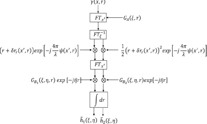
2Ωx )]. From Eqs. (45) and (47), efficient computation ofh1(ξ, η) andh2(ξ, η) is easily

attainable. Figure 5 summaries the computation flow chart of the procedures outlined above. It should be stated that at this point that since the attitude variations follows the condition in Equation (21), the validity limit of the simulator in domain of attitude variations is specified by Eq. (37). It follows that

δaz(x) X

r+δrr(x, r) <

X r =

λ

L. (48)

The validity limit of the simulator with respect to trajectory deviations should satisfy Eqs. (11), (12) and (40). Note that condition in Eq. (11) implicitly requires the topography be smooth, which implies that condition in Eq. (40) is established [26]. Then the approximations made in the proposed approach for trajectory deviations only satisfy the conditions of Eqs. (11) and (12), which are the same as the analysis of [27]. Together with condition in Eq. (37), the proposed approach in Section 3.2 is valid for moderate trajectory deviations and antenna pointing error.

3.3. Computational Efficiency Comparison

Now, comparison of computational complexity between the approaches presented in Sections 3.1 and 3.2 is in order, where the computational complexity, for both approaches, is increased as the nth order

approximation of the two-way antenna radiation diagram. Denoting Nx andNr the azimuth and range directions (in pixels), respectively, of the raw signal, then the computational complexity of γ(x, r) is of the order NxNr. Let N and N1 be the complex multiplications needed by the method discussed in

Section 3.1 and the one in Section 2.1 [26], then

N = (n+ 1)N1. (49)

From [27], it is known that

N1 ≈NxNr(1 + log2NxNr). (50)

Now, let N and N2 be the complex multiplications (in pixels) needed by the method discussed in Section 3.2 and the one in Section 2.2, then

˜

N = (n+ 1)N2 (51)

where

N2≈NxNr2. (52)

From Eqs. (49) and (51), it can be seen that the algorithm given in Section 3.1 has a higher computational efficiency than the one discussed on Section 3.2 with the samen. Now let us compare the computational complexity of the proposed approach of Section 3.2 with reference to the time-domain approach. It is not difficult to verify that the computational complexity in the time domain is [27]:

N3 ≈NxNrNtpNsa (53)

whereNtpandNsaare the dimensions of the transmitted pulse and of the synthetic aperture. In general,

the size ofn is smaller than Nsa and Ntp is of the same order as Nr [27], then the algorithm shown in

Section 3.2 turns out to have a higher computational efficiency than the exact time domain approach. The computational time saving is

N3 N ≈

Nsa

n+ 1. (54)

Hence, simulation of raw signal from extended scenes becomes highly feasible in the sense of saving computation time.

4. SIMULATION RESULTS

In this section, some simulation results are presented to verify the effectiveness of the proposed approaches. Simulation parameters were taken from the X-band airborne SAR system [26] and [27], given in Table 2. Note that the ideal time domain simulator can be realized by making use of equation of Eq. (19). For shorthand notation, we designate the algorithm presented in Section 3.1 as Algorithm A, the algorithm in Section 3.2 as Algorithm B, and the time-domain approach as Algorithm C. Considering that the raw signal from a scattering point is placed at midrange (r= 5140 m) over a perfectly absorbing background, the horizontal and vertical components of the trajectory deviations are reported in Figure 6. The antenna pointing error is assumed, without loss of generality, to be sinusoidal form:

δaz(x) =δmsin

2π vTbx

_{+φ0 (55)}

whereδm is the amplitude, Tb the antenna jitter period, andφ0 the initial phase, assumingδm = ₂₀1 _Lλ,

Tb = 101 Ts and φ0 = 0. The simulation results of Approaches A and C are compared, where the

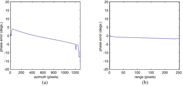
amplitude comparisons of the target along the azimuth and range direction are plotted in Figures 7(a) and (b), respectively. It can be observed that the difference between the exact and simulated raw signal is negligible. Comparison of phase in the azimuth and range directions is shown in Figure 8, where Figure 8(a) is the azimuth cut while Figure 8(b) is the range cut. We see that the phase difference between Algorithms A and C is very small. Thus the accuracy of Algorithm A is verified.

Table 2. Simulated sensor parameters.

Nominal height 4000 m Range pixel dimension 3 m

Midrange coordinate 5140 m Chirp bandwidth 45 MHz

Wavelength 3.14 cm Chirp duration 5µs

Platform velocity 100 m/s Azimuth antenna dimension 1 m

Pulse Repetition Frequency 400 Hz Range antenna dimension 8 cm

Sampling Frequency 50 MHz Number of azimuth samples in the raw data 1941

Azimuth pixel dimension 25 cm Number of range samples in the raw signals 830

400 800 1200 1600 2000

-3 -2 -1 0 1 2 3

azimuth pixels

trajectory deviation [cm]

Horizontal displacement

Vertical displacement

Figure 6. The horizontal and vertical displacement of trajectory deviations [cm] vs. the azimuth pixels.

0 400 800 1200

0 0.2 0.4 0.6 0.8 1

azimuth (pixels)

amplitude

0 100 200 300 400 500 600 700 800 900 0

0.2 0.4 0.6 0.8 1 1.2

range (pixels)

amplitude

(a) (b)

Figure 7. SAR raw data amplitude comparison between Algorithm A and C (The blue lines are the results from the Algorithm A, and the red lines are from Algorithm C).(a) Azimuth cut. (b) Range cut. The scattering point is located at the center of the illuminate scene.

respectively. It is seen from the figures that the difference, both the amplitude and phase, between exact and the simulated raw signal is very small.

0 200 400 600 800 1000 1200 -20

-15 -10 -5 0 5 10 15 20

azimuth (pixels)

phase error (degs.)

0 50 100 150 200 250

-20 -15 -10 -5 0 5 10 15 20

range (pixels)

phase error (degs.)

(a) (b)

Figure 8. SAR raw data phase comparison between Algorithm A and C. (a) Azimuth cut. (b) Range cut. The scattering point is located at the center of the illuminated scene.

200 400 600 800 1000120014001600 1800 2000 -0.2

0 0.2 0.4 0.6 0.8 1

azimuth pixels

trajectory deviation [m]

Horizontal displacement

Vertical displacement

Figure 9. The horizontal and vertical displacement of trajectory deviations [m] vs. the azimuth pixels.

0 400 800 1200

0 0.2 0.4 0.6 0.8 1

azimuth (pixels)

amplitude

0 100 200 300 400 500 600 700 800 0

0.2 0.4 0.6 0.8 1

range (pixels)

amplitude

(a) (b)

0 200 400 600 800 1000 1200 -20

-15 -10 -5 0 5 10 15 20

azimuth (pixels)

phase error (degs.)

0 50 100 150 200 250

-20 -15 -10 -5 0 5 10 15 20

range (pixels)

phase error (degs.)

(a) (b)

Figure 11. SAR raw data phase comparison between Algorithm B and C. (a) Azimuth cut. (b) Range cut. The scattering point is located at near range at r= 4840 m.

0 500 1000 1500 2000

-8 -6 -4 -2 0 2 4 6

azimuth pixels

trajectory deviation [m]

vertical displacement

Honrizontal displacement

Figure 12. Simulated trajectory deviations relative to Figure 13 and Figure 14.

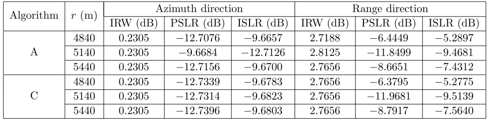
Table 3. The focus performance of the point target response of Algorithm A and C.

Algorithm r (m) Azimuth direction Range direction

IRW (dB) PSLR (dB) ISLR (dB) IRW (dB) PSLR (dB) ISLR (dB)

A

4840 0.2305 −12.7076 −9.6657 2.7188 −6.4449 −5.2897

5140 0.2305 −9.6684 −12.7126 2.8125 −11.8499 −9.4681

5440 0.2305 −12.7156 −9.6700 2.7656 −8.6651 −7.4312

C

4840 0.2305 −12.7339 −9.6783 2.7656 −6.3795 −5.2775

5140 0.2305 −12.7314 −9.6823 2.7656 −11.9681 −9.5139

5440 0.2305 −12.7396 −9.6803 2.7656 −8.7917 −7.5640

0 400 800 1200 0

0.2 0.4 0.6 0.8 1

azimuth (pixels)

amplitude

0 100 200 300 400 500 600 700 800 0

0.2 0.4 0.6 0.8 1

range (pixels)

amplitude

(a) (b)

Figure 13. SAR raw data amplitude comparison between Algorithm B and C. The track deviations are depicted in Figure 12 and (55) gives the antenna pointing errors (The blue lines are for the results of Algorithm B and the red lines are from Algorithm C). (a) Azimuth cut. (b) Range cut. The scattering point is located in the near range atr = 4840 m.

0 200 400 600 800 1000 1200 -20

-15 -10 -5 0 5 10 15 20

azimuth (pixels)

phase error (degs.)

0 50 100 150 200 250

-20 -15 -10 -5 0 5 10 15 20

range (pixels)

phase error (degs.)

(a) (b)

Figure 14. SAR raw data phase comparison between Algorithm B and C. The track deviations are depicted in Figure 12 and (55) gives the antenna pointing. (a) Azimuth cut. (b) Range cut. The scattering point is located in the near range at r= 4840 m.

amplitude and phase error in the azimuth direction between Algorithms B and C. It can be observed that both the amplitude and phase error are very large. Therefore, Algorithm B is only applied to moderate trajectory deviations and azimuth antenna pointing errors.

By comparing Algorithm A with Algorithm C, the point target analyses for far range (5440 m), midrange (5140 m) and near range (4840 m) are shown in Table 3, including the impulse response width (IRW), peak side-lobe ratio (PSLR) and integrated side-lobe ratio (ISLR). It is shown that the proposed algorithms achieve high precision as that in time domain. Similar conclusion can be obtained by comparing Algorithm B with Algorithm C, which is shown in Table 4.

final images obtained by processing the simulated raw signal using Algorithm A and Algorithm B without motion compensation (MOCO) are shown in Figures 17(a) and (b), respectively. And yet, the corresponding trajectory deviations MOCO results of Algorithms A and B, which are shown in [33], are displayed in Figures 7(c) and (d), respectively.

0 400 800 1200

0 0.2 0.4 0.6 0.8 1

azimuth (pixels)

amplitude

0 200 400 600 800 1000 1200 -40

-30 -20 -10 0 10 20 30 40

azimuth (pixels)

phase error (degs.)

(a) (b)

Figure 15. SAR raw data amplitude comparison between Algorithm B and C. The track deviations are depicted in Figure 9, (55) gives the antenna pointing errors where δm = _Lλ (The blue lines are for the results of Algorithm B and the red lines are from Algorithm C). (a) Azimuth amplitude error. (b) Azimuth phase error. The scattering point is located in the midrange at r= 5140 m.

Table 4. The focus performance of the point target response of Algorithm B and C.

Algorithm r (m) Azimuth direction Range direction

IRW (dB) PSLR (dB) ISLR (dB) IRW (dB) PSLR (dB) ISLR (dB)

B

4840 0.2266 −5.0346 −3.9095 2.7188 −6.8351 −5.6503

5140 0.2227 −3.4025 −2.2344 2.8125 −12.3214 −9.5441

5440 0.2188 −2.4523 −1.2622 2.7656 −8.5 −7.2288

C

4840 0.2266 −5.3933 −4.2801 2.7656 −7.1473 −6.0101

5140 0.2227 −3.3611 −2.1945 2.7656 −12.8208 −9.6497

5440 0.2188 −2.4399 −1.2496 2.7656 −8.0237 −6.8483

400 800

-3 -2 -1 0 1 2 3

azimuth pixels

trajectory deviation [cm]

Horizontal displacement

Vertical displacement

0 100 200 300 400 500 600 700 800 900 -0.4

-0.2 0 0.2 0.4 0.6 0.8 1

azimuth pixels

trajectory deviation [m]

vertical displacement

Honrizontal displacement

(a) (b)

range

azimuth

range

azimuth

range

azimuth

range

azimuth

(a) (b)

(c) (d)

Figure 17. Image comparison of different algorithms: (a) Algorithm A without motion compensation. (b) Algorithm B without motion compensation. (c) Algorithm A with the compensation of trajectory deviations. (d) Algorithm B with the compensation of trajectory deviations.

5. CONCLUSIONS

In this paper, the problem of efficient airborne SAR raw signal simulation is addressed for sensor trajectory deviations and antenna pointing errors for stripmap SAR mode. Under the assumption that the antenna pointing error is small compared with the beamwidth, the raw signal is separated into three different components, where the first one describes the trajectory deviations, and the latter two account for the effect of trajectory deviations and antenna pointing error. Consequently, an efficient algorithm for SAR raw signal simulation in the presence of moderate trajectory deviations and antenna pointing errors is proposed. The simulation approach to evaluation of each component relies on using 1-D azimuth Fourier domain processing followed by range time domain integration. This approach has a high computational efficiency compared with the time domain simulator due partly to the use of FT in the azimuth direction, while maintain high accuracy. Extensive analytical and numerical evaluations are performed to demonstrate the effectiveness and efficiency of the proposed algorithms. It should be worth to test the algorithms on real world data from airborne SAR system and will be reported in the future.

ACKNOWLEDGMENT

APPENDIX A.

Let us conside Eq. (36). By comparingδrxr(x, x, r) and δrr(x, r), we can obtain

δrxr(x, x, r)−δrr(x, r)≈ −d(x) sin(ϑ(x, r)−β(x)) +d(x) sin(ϑ(x, r)−β(x)) =−d(x)[sin(ϑ(x, r) cosβ(x))−cosϑ(x, r) sinβ(x)]

+d(x)[sinϑ(x, r) cosβ(x)−cosϑ(x, r) sinβ(x)] = sinϑ(x, r)[−d(x) cosβ(x) +d(x) cosβ(x)]

+ cosϑ(x, r)[d(x) sinβ(x)−d(x) sinβ(x)]. (A1) Since 0<|ϑ(x, r)|< π₂, the approximation of δrxr(x, x, r)≈δrr(x, r) requires the following conditions

are satisfied:

d(x) cosβ(x) = d(x) cosβ(x) (A2)

d(x) sinβ(x) = d(x) sinβ(x). (A3)

The corresponding square on both sides of Equations (A2) and (A3) are

d2(x) cos2β(x) = d2(x) cos2β(x) (A4)

d2(x) sinβ2(x) = d2(x) sin2β(x). (A5)

By adding the both sides of Equations (A4) and (A5), it can get

d2(x) =d2(x) (A6) then Eq. (36) is obtained.

REFERENCES

1. Franceschetti, G. and G. Schirinzi, “A SAR processor based on two-dimensional FFT codes,”IEEE Trans. Aerosp. Electron. Syst., Vol. 26, No. 2, 142–149, 1990.

2. Kulpa, K., P. Samczy´nski, M. Malanowski, A. Gromek, D. Gromek, W. Gwarek, B. Salski, and G. Ta´nski, “An advanced SAR simulator of three-dimensional structures combining geometrical optics and full-wave electromagnetic methods,”IEEE Trans. Geosci. Remote Sens., Vol. 52, No. 1, 776–784, 2014.

3. Franceschetti, G., A. Iodice, D. Riccio, and G. Ruello, “SAR raw signal simulation for urban structures,”IEEE Trans. Geosci. Remote Sens., Vol. 41, No. 9, 1986–1995, 2003.

4. Balz, T. and U. Stilla, “Hybrid GPU-based single- and double-bounce SAR simulation,” IEEE

Trans. Geosci. Remote Sens., Vol. 47, No. 10, 3519–3529, 2009.

5. Dumont, R., C. Guedas, E. Thomas, F. Cellier, and G. Donias, “DIONISOS. An end-to-end SAR simulator,” Proc. EuSAR, 677–680, 2010.

6. Mametsa, H. J., F. Rouas, A. Berges, and J. Latger, “Imaging radar simulation in realistic

environment using shooting and bouncing rays technique,” Proc. SPIE, SAR Image Analysis,

Modeling and Techniques IV, 34–40, 2001.

7. Margarit, G., J. J. Mallorqui, J. M. Rius, and J. Sanz-Marcos, “On the usage of GRECOSAR, an orbital polarimetric SAR simulator of complex targets, to vessel classification studies,” IEEE Trans. Geosci. Remote Sens., Vol. 44, No. 12, 3517–3526, 2006.

8. Hammer, H., T. Balz, E. Cadario, U. Soergel, U. Thoennessen, and U. Stilla, “Comparison of SAR simulation concepts for the analysis of high resolution SAR data,”Proc. EuSAR, 2008.

9. Anglberger, H., R. Speck, T. Kampf, and H. Suess, “Fast ISAR image generation through localization of persistent scattering centers,” Proc. SPIE Defence, Security and Sensing, 2009. 10. Auer, S., S. Hinz, and R. Bamler, “Ray-tracing simulation techniques for understanding

high-resolution SAR images,” IEEE Trans. Geosci. Remote Sens., Vol. 48, No. 3, 1445–1456, 2010. 11. Brunner, D., G. Lemoine, H. Greidanus, and L. Bruzzone, “Radar imaging simulation for urban

12. Smolarczyk, M., “Radar signal simulator for SAR algorithms tests,” Proc. International Radar Symposium, 509–513, Dresden, Germany, 2003.

13. Kulpa, K., M. Smolarczyk, G. Ta´nski, A. Gromek, and P. Jobkiewicz, “Radar signal simulator and its usage for interferometric SAR radars phase unwrapping algorithms test,”15th IEEE Int. Conf., 427–430, MIKON, 2004.

14. Horst, H., K. Silvia, and S. Karsten, “On the use of GIS data for realistic SAR simulation of large urban scenes,”IGARSS, 4538–4541, 2015.

15. Liu, B. C. and Y. J. He, “SAR raw data simulation for ocean scenes using inverse Omega-K algorithm,”IEEE Trans. Geosci. Remote Sens., Vol. 54, No. 10, 6151–6169, 2016.

16. Blacknell, D., A. Freeman, S. Quegan, A. I. Ward, P. I. Finley, H. C. Oliver, G. R. White, and J. W. Wood, “Geometric accuracy in airborne SAR image,”IEEE Trans. Aerosp. Electron. Syst., Vol. 25, No. 2, 241–258, 1989.

17. Oliver, J. C., “Review article — Synthetic aperture radar imaging,” Phys. D: Applied Physics, Vol. 22, No. 7, 871–890, 1989.

18. Mori, A. and F. De Vita, “A time-domain raw signal simulator for interferometric SAR,” IEEE Trans. Geosci. Remote Sens., Vol. 42, No. 9, 1811–1817, 2004.

19. Xu, F. and Y. Jin, “Imaging simulation of polarimetric SAR for a comprehensive terrain scene using the mapping and projection algorithm,”IEEE Trans. Geosci. Remote Sens., Vol. 44, No. 11, 3219–3234, 2006.

20. Eldhuset, K., “High resolution spaceborne INSAR simulation with extended scenes,” Proc. Inst. Elect. Eng.-Radar Sonar Navig., 53–57, 2005.

21. Khwaja, S. A., L. Ferro-Famil, and E. Pottier, “Efficient SAR raw data generation for anisotropic urban scenes based on inverse processing,”IEEE Geosci. Remote Sens. Lett., Vol. 6, No. 4, 757–761, 2009.

22. Franceschetti, G., M. Miliaccio, D. Riccio, and G. Schirinzi, “SARAS: A SAR raw signal simulator,” IEEE Trans. Geosci. Remote Sens., Vol. 30, No. 1, 110–123, 1992.

23. Khwaja, S. A., L. Ferro-Famil, and E. Pottier, “SAR raw data simulation in the frequency domain,” Proc. The 3rd European Radar Conferene, 277–280, 2006.

24. Franceschetti, G., M. Miliaccio, and D. Riccio, “SAR simulation of actual ground sites described in terms of sparse input data,”IEEE Trans. Geosci. Remote Sens., Vol. 32, No. 6, 1600–1169, 1994. 25. Franceschetti, G., A. Iodice, M. Migliaccio, and D. Riccio, “A novel across-track SAR interferometry

simulator,” IEEE Trans. Geosci. Remote Sens., Vol. 36, No. 3, 950–962, 1998.

26. Franceschetti, G., A. Iodice, S. Perna, and D. Riccio, “SAR sensor trajectory deviations: Fourier

domain formulation and extended scene simulation of raw data,” IEEE Trans. Geosci. Remote

Sens., Vol. 44, No. 9, 2323–2334, 2006.

27. Franceschetti, G., A. Iodice, S. Perna, and D. Ricco, “Efficient simulation of airborne SAR raw data of extended scenes,”IEEE Trans. Geosci. Remote Sens., Vol. 44, No. 10, 2851–2860, 2006. 28. Tang, X., M. Xiang, and L. Wei, “SAR raw signal simulation accounting for antenna attitude

variations,” IGARSS, 613–616, 2009.

29. Vandewal, M., R. Speck, and H. S¨uß, “Efficient SAR raw data generation including low squint angles and platform instabilities,” IEEE Geosci. Remote Sens. Lett., Vol. 5, No. 1, 26–30, 2008. 30. Khwaja, A. S., L. Ferro-Famil, and E. Pottier, “Efficient stripmap SAR raw data generation taking

into account sensor trajectory deviations,”IEEE Geosci. Remote Sens. Lett., Vol. 8, No. 4, 794–798, 2011.

31. Franceschetti, G., R. Lanari, and S. Marzouk, “A new two-dimensional squint mode SAR processor,”IEEE Trans. Aerosp. Electron. Syst., Vol. 32, No. 2, 854–863, 1996.

32. Chen, K. S.,Principles of Synthetic Aperture Radar — A System Simulation Approach, CRC Press, 2015.