Carlo A. Gonano*, Riccardo E. Zich, and Marco Mussetta
Abstract—Dealing with the project of metamaterials scientists often have to design circuit elements at a sub-wavelength (or “microscopic”) scale. At that scale, they use the set of Maxwell’s equations in free-space, and neither permittivity ε nor permeability μare formally defined. However, the objective is to use the unit cells in order to build a bulk material with some desired “macroscopic” properties. At that scale the set of Maxwell’s equations in matter is adopted. To pass from one approach to the other is not obvious. In this paper we analyse the classic definitions of polarizationP and magnetization M, highlighting their limits. Then we propose a definition for P and M fully consistent with Maxwell’s equations at any scale.
1. INTRODUCTION
Maxwell’s equations are the well-known fundamental laws describing the ElectroMagnetic field [1]. Depending on the system, they can be written in “free-space” or in “matter”. Usually, if you are dealing with a “microscopic” system, you use free-space Maxwell’s equations. Otherwise, if the system is composed by “macroscopic” bulk materials, you have to use the Maxwell’s equations in matter.
In the field of metamaterials [2–4], engineers often have to project small, “microscopic”, sub-wavelength unitary cells in order to create a “macroscopic” bulk material with some desired properties. Designing the sub-wavelength circuit or device, you have to deal with free-space Maxwell’s equations, while if you want to describe the macroscopic behaviour you are going to use the in-matter set. So the problem of how to council the two different models (approaches), microscopic and macroscopic ones, arises [5]. In particular, polarizationP and magnetizationM fields should be rigorously defined in order to avoid paradoxes and contradictions.
In the first part of this work we make a comparison between the two sets of Maxwell’s Equations, in free-space and in matter respectively, and we derive a third set in order to enlighten the role of P
and M.
In the second part we explore the limits of the distinction between “free” and “bound” charges and currents.
In the third part of this work we analyse the classic definitions of P and M, showing they cannot be easily extended to the microscopic case.
In the fourth and fifth parts we fix some conditions and then formally define polarization P and magnetization M for a generic system, no matter if “microscopic” or macroscopic”, in a scale-invariant way.
In the sixth we discuss the main results and in the seventh part we resume some conclusions.
Received 6 October 2015, Accepted 9 November 2015, Scheduled 12 November 2015
* Corresponding author: Carlo Andrea Gonano ([email protected]).
2. COMPARISON OF MAXWELL’S EQUATIONS SETS 2.1. Maxwell’s Equations in Free Space in the Time Domain
Maxwell’s Equations in free-space or in “vacuum” can be written as:
⎧ ⎪ ⎪ ⎨ ⎪ ⎪ ⎩
− →
∇T·ε0E=ρe
− →∇ × 1
μ0B =Je+ ∂
ε0E
∂t
⎧ ⎨ ⎩
− →∇T·
B = 0 −
→∇ ×
E =−∂ B
∂t
(1)
where: E is the electric field;B is the magnetic (induction) field;ρe is the electric charge density;Je is the electric current per unit of surface; ε0 and μ0 are the free space electric permittivity and magnetic permeability respectively. Here we adopt the superscript T to indicate the transposed (horizontal) vectors and−→∇, ensuring consistency with further matrix equations.
2.2. Maxwell’s Equations in Matter in the Time Domain
Maxwell’s Equations in matter have a similar structure to free-space ones, but they involve the displacement field D, the magnetic field H, and free charge ρf and current Jf densities. All of these have to be expressed in terms of⎧ E and B via the constitutive relations in order to be tackled.
⎨ ⎩
− →
∇T·D =ρ f −
→∇ ×
H =Jf +∂ ∂tD
⎧ ⎨ ⎩
− →
∇T·B = 0 −
→∇ ×
E =−∂ B
∂t
(2)
The second pair of equations is the same for the two sets, and it can be rephrased in terms of scalarϕA
and vector A potentials. ⎧
⎨ ⎩
B =−→∇ ×A
E =−∂ A
∂t −
− →∇
ϕA
(3)
2.3. Maxwell’s Equations for P and M
Now we focus the attention on the sets involving thesources of the EM fields, and we will try to derive an analogous set in order to enlighten the polarization P and magnetizationM. The sources of the EM fields are electric charges and currents, and usually they are divided in free and bound ones:
ρe = ρf +ρb (4)
Je = Jf +Jb (5)
The displacement D and magnetic H fields are related through their own definitions to P and M
respectively, in fact:
Dε0E +P =⇒ ε0E =D −P (6)
H 1
μ0B −M =⇒
1
μ0B =H +M (7)
where the symbolstands for “is defined to be equal to”. Subtracting the first sets of (1) and (2) one from the other, we obtain the Maxwell’s Equations forP and M:
⎧ ⎨ ⎩
− →∇T·
(−P) =ρb −
→∇ ×
M =Jb+∂(−
P)
∂t
(8)
Free charges are those free to move, instead of bound ones which have limited displacements.
This could be a reasonable definition [6–9], since in metals and conductors electrons can move quite easily in the crystal lattice. In polarized dielectrics, instead, the charges are restrained by strong internal forces and so they are bound to their position. However, that definition does not work in some contexts.
Let’s consider a plasma, that is a ionized gas of charged unbound particles [10]. Formally, all the charges are free, since the molecular forces are negligible and the conductivity is very high. At a microscopic level — that in this case correspond to sizes smaller than the Debye’s length λD — the plasma is thus usually modelled as system of free charged particles.
ΔxλD =⇒system of free charged particles (9)
However, charges produce and are subjected to the EM forces. At a macroscopic level, that is for systems larger than λD, the plasma is modelled as a continuous medium with average properties. For example, in the Drude model [11] it is possible to calculate the effective permittivityεof the plasma as:
ε(ω)
ε0 = 1− ω2P
ω2 (10)
whereωP is the characteristic plasma “frequency”. SinceD(ω) =ε(ω)E(ω), the polarization of plasma can be different from zero, in fact:
P(ω) = (ε(ω)−ε0)E(ω) (11)
Since P =0 , except as ω → ∞, both ρb and Jb can be different from zero and so the plasma can contain bound charges.
ΔxλD =⇒continuous system with bound charges (12)
Also in this case the distinction between free and bound charges seems to be related to thescale of the system.
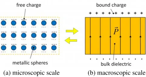
Let’s now make an other example. Consider a group of metallic spheres: if they are invested by an electric field, there will be a displacement of free charges on the single surfaces (see Fig. 1). If we look at the same system at a larger scale, interpreting the group of spheres as a bulk metamaterial, then the displacement of charges looks quite limited. Actually, they are bound on the surface of the little spheres and cannot move far beyond. Actually, at that macroscopic scale the system looks as a polarized dielectric.
3.2. Free Charges as Charges in Conductors
An alternative definition of free charge could be based on the distinction between conductors and dielectrics:
Free charges and currents are those in conductors (metals), instead of bound ones which are in dielectrics.
(a) microscopic scale (b) macroscopic scale
Figure 1. (a) At a microscopic scale, the charge on the single metallic spheres is regarded as free; (b) At macroscopic scale, the same system looks as a polarized dielectric since the charges are bound and their displacements are small.
(a) (b) (c)
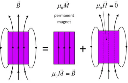
Figure 2. (a) At a microscopic scale, a magnet can be modelled through Amperian loops of bound
current; (b) Magnetic field produced by a permanent magnet; (c) Hysteresis curve. AtH= 0 there are residualB field and a net magnetization M.
Let’s consider a static permanent magnet: it generates a magnetic fieldB even if there are no visible macroscopic currents. However, a magnet is usually modelled as an ensemble of microscopic current loops (Amperian currents, see Fig. 2). Many permanent magnets are made of conducting materials, like iron, cobalt, nickel etcetera, so the currents inside the magnet should be free. Hence, bound currents should be negligible: |Jb| |Jf|. Surprisingly, that’s false, and the opposite is true.
In the static case (∂.∂t = 0), H and M can be calculated as: −
→
∇ ×H =Jf; →−∇ ×M =Jb (13)
Since we are considering a permanent magnet with no external currents, theH field inside is zero (see Fig. 3) and the magnet will produce a residual B field which can be determined from the hysteresis curve at H = 0. In other words, inside the permanent magnet the H field is much smaller than the magnetization M, and so the free currents are much less intense than bound ones:
inside permanent magnet |H| |M|=⇒ |Jf| |Jb| (14) Thus, even if the permanent magnet is made of a conducting material, the currents generating its magnetic field B are not free, but bound ones. Differently, the magnetization field M would be identically null.
The case of a empty inductor filled with current (Fig. 4) can be regarded as complementary to the permanent magnet. The current flowing in the windings is usually considered asfree (soJe =Jf) and since the inductor is empty inside, its magnetization M is actually zero: M =0. Field H instead is comparable toB/μ0:
Figure 3. Fields for a permanent magnet. The
H field is zero inside, while the magnetization M
is high and equal to B/μ0.
Figure 4. Fields for an empty inductor. The magnetization M is zero inside the solenoid, since it is empty, while the H field is equal to
B/μ0. This case is complementary to that of the permanent magnet.
Summarizing:
Inside a permanent magnet B =μ0M; H =0 =⇒Je=Jb (16)
Inside an empty inductor B =μ0H; M =0 =⇒Je=Jf (17)
3.3. Concluding Remarks on Free and Bound Charges
As we have seen in the previous paragraphs, to distinguish free charges from bound ones is not so obvious and that subdivision appears to rely on the system to be analysed, and in particular on its scale. Generally speaking, at microscopic scales charges look to be free and discrete, while at macroscopic scales they appear to be bound and continuous. Moreover, in numerical simulation free charges and currents are considered instead as theknown orassigned sources for the ElectroMagnetic problem. On the contrary, bound charges and currents are considered as unknown variables to be calculated, once the constitutive relations for the media are assigned.
Shortly, the concepts of free and bound charges sound quite fuzzy and arbitrary, and trying to impose a rigid definition of them seems useless. Actually scientists working on different topics will adopt different definitions, suitable to their models and objectives. Here we do not mean to re-define free and bound charges, but if we want to develop and work with coherent models we must know the objects we are dealing with. Otherwise, we risk to achieve contradictory conclusions and misleading results, without being aware of that.
Hereafter we assume thefree and bound charges have been defined in some way by the “user”: we are just going to require that Maxwell’s Equations have to be satisfied.
3.4. Conservation of Charge
It could be easily verified that electric charges are conserved for each set in (3), (8). Let’s consider the “microscopic” case: we take the derivative in time for the divergence of E, apply the divergence to the curl ofB (identically zero) and then sum the equations together:
⎧ ⎪ ⎪ ⎪ ⎨ ⎪ ⎪ ⎪ ⎩
∂ ∂t
−→
∇T·ε0E
= ∂
∂tρe
0 =−→∇T·
− →∇ × 1
μ0B
=−→∇T·
⎛ ⎝Je+∂
ε0E
∂t
⎞ ⎠=⇒
(18)
∂ρe
∂t +
− →
With an analogous procedure, conservation laws forfree and bound charge can be deduced:
∂ρf
∂t +
− →∇T·
Jf = 0 conservation of free charge (20)
∂ρb
∂t +
− →∇T·
Jb= 0 conservation of bound charge (21)
3.5. Fields Produced by Free and Bound Charges
Thanks to the linearity of Maxwell’s Equations, we can consider separately free charges from bound ones and decompose the fields E and B on the basis of their sources. We call:
• Ef, Bf, Af, ϕA,f the fields produced byfree charges and currents. • Eb, Bb, Ab, ϕA,b the fields produced bybound charges and currents. The Maxwell’s Equations for free charges will look so:
⎧ ⎪ ⎪ ⎨ ⎪ ⎪ ⎩
− →∇T·
ε0Ef
=ρf
− →∇ × 1
μ0Bf =Jf + ∂
ε0Ef
∂t
⎧ ⎨ ⎩
Bf =−→∇ ×Af
Ef = −∂ ∂tAf −−→∇ϕA,f
(22)
In the same way, for bound charges will hold:
⎧ ⎪ ⎪ ⎨ ⎪ ⎪ ⎩
− →∇T·
ε0Eb
=ρb
− →∇ × 1
μ0Bb =Jb+ ∂
ε0Eb
∂t
⎧ ⎨ ⎩
Bb =−→∇ ×Ab
Eb =−∂ ∂tAb −−→∇ϕA,b
(23)
The sets (22) and (23) are quite similar to (2) and (8) respectively. In fact, the sources of the fields are unchanged. Summing together the equations in (22) with those in (23) we get the set of Maxwell’s Equations in vacuum (1). Obviously the global fields produced by all charges and currents ρe and Je will be the sum of those originated by free and bound ones.
E = Ef +Eb ϕA=ϕA,f +ϕA,b (24)
B = Bf +Bb A =Af +Ab (25)
It should be noticed that all the fields in (22) and (23) can propagate also in vacuum, while P
and M are identically zero in empty space. In fact, in vacuum the permittivity and permeability are respectivelyε0 and μ0, so:
D = ε0E =⇒P =D −ε0E =0 (26)
H = 1
μ0B =⇒M =−H +
1
μ0B =0 (27)
In general,P andM are required to be zero outside any body.
4. ANALYSING THE CLASSIC DEFINITIONS FOR P AND M
(a) microscopic scale (b) macroscopic scale
Figure 5. (a) At microscopic scale, the polarization field P among the charged particles should be zero, since that space is vacuum (ε= ε0); (b) At macroscopic scale, the same system looks as a bulk material with a non-zero polarization field P.
4.1. Limits of Classic Definition for Polarization P
Classically [6–9, 12] the polarization P on the domain Ωx is defined as the net electric dipole per unit of volume V. If all the electric dipoles pi on Ωx are known, thenP is:
P = 1
V
Ωx
(pi) (28)
Unfortunately, with this definition P is not a field P(x, t), but an average quantity: in fact it is not associated to a pointx, but to a whole domain Ωx.
Let’s suppose we consider a system at microscopic scale, made by many charged particles separated from vacuum (Fig. 5). What is the polarization fieldP(x, t) on this domain Ωx? Since in vacuum holds
D=ε0E, rigorouslyP(x, t) should be zero wherever there are no charges.
P(x, t) =0 ∀x∈ vacuum (29)
However, if we consider the same system at a larger scale, we could see a bulk material with net dipole and polarization. So definingP appears to be again a scale question.
4.2. Calculating a Net Electric Dipole
Another problem to face in defining P, also as an average quantity, is how to calculate the net dipole on a domain.
For a group of point chargesQi, the net dipolep is equal to:
p= i
pi = i
Qi·(xi−x0) (30)
wherexi is theith charge position, whilex0 is the reference point. More generally, for a domain Ωx the net electric dipolep can be calculated as:
p=
Ωx
ρ·(x−x0)dΩx (31)
The problem resides in the arbitrary pointx0: if the net chargeQon the domain is different from zero, the value of p can change depending on the choice ofx0, in fact:
Q=
Ωx
ρ dΩx=⇒p=
Ωx
(ρ·x)dΩx−Q x0 (32)
Supposing the pointx0 is fixed, holding (28), (31) the average polarization can be written as:
P = 1
V
Ωx
ρ·(x−x0)dΩx (33)
Now we are going to analyse the limits of the definition for magnetization M, following an analogous procedure.
4.3. Limits of Classic Definition for Magnetization M
Classically [6–9, 12], the magnetization M on the domain Ωx is defined as the net magnetic dipole per unit of volumeV. If all the magnetic dipolesmi on Ωx are known, thenM is:
M = 1
V
Ωx
(mi) (34)
Similarly to (28), that quantity is not a field M(x, t) but an average value: in fact it is not associated to a pointx, but to a whole domain Ωx.
Let’s suppose we consider a system at microscopic scale, made by many circular current loops (amperian currents). What is the magnetization fieldM(x, t) on this domain Ωx?
Since in vacuum holdsH = μ1
0B, rigorouslyM(x, t) should be zero wherever there are no currents.
M(x, t) =0 ∀x∈ vacuum (35)
However, if we consider the same system at a larger scale, we could see a bulk material with net dipole and magnetization. For example, it could be an ordinary magnet. So definingM appears to be also a
scale question.
4.4. Calculating a Net Magnetic Dipole
Another problem to face in definingM, also as an average quantity, is how to calculate the net magnetic dipole on a domain.
For a group of point chargesQi, the net magnetic dipolem is equal to:
m= 1
2
i
(xi−x0)×(Qivi) (36)
wherexi is the ith charge position,vi is its velocity andx0 is the reference point. More generally, for a domain Ωx net magnetic dipole m can be calculated as:
m= 1
2
Ωx
(x−x0)×(ρv)dΩx= 1 2
Ωx
(x−x0)×J d Ωx (37)
Even in this case, the value ofm can change depending on the choice of reference pointx0, so it is not uniquely defined. Supposingx0 to be fixed, holding (34), (37) theaverage magnetization can be written as:
M = 1
V
1 2
Ωx
(x−x0)×J d Ωx (38)
5. CONDITIONS FOR THE DEFINITION OF P AND M
Now we are going to give two definitions, one for polarization M, one for magnetization P, requiring that these respect some conditions:
• bothP andM must satisfy Maxwell’s Equations inside any material Ωx, that is:
⎧ ⎨ ⎩
− →∇T·
(−P) =ρb −
→∇ ×
M =Jb +∂(−
P)
∂t
Ωx Ωx
• Moreover, the definitions forP andM must be valid for any kind of materials, even for a non-linear or hysteretic one.
We cannot guarantee a priori that all these requirements can be accomplished, but we are going to verify if that is possible or not.
5.1. Bound Charges and Currents are Null Outside Materials
Here we prove that, holding conditions (39) and (40), bound charges and currents are identically zero
outside any material Ωx. In fact:
P =0
M =0 ∀x /∈Ωx=⇒
⎧ ⎨ ⎩
− →∇T·
(−0) =ρb −
→∇ ×
0 =Jb+∂(∂t−0) =⇒
ρb = 0
Jb =0 ∀x /∈Ωx (42)
So the bound charges and currents ρb and Jb can exist just inside the material Ωx or at least on its boundary∂Ωx.
5.2. Consistency for P Definition
Here we check if the classic definition ofP as average quantity is coherent with Maxwell’s Equation (39). We take the equation linking the divergence forP toρband try to derive the electric dipole’s definition.
− →∇T·(−
P) = ρb (43)
−→
∇T·P·(x−x0) = −ρ
b·(x−x0) (44)
Δx·
−→
∇T·P = −ρb·Δx (45)
We place Δx=x−x0 in order to simplify the notation, and exploit a differential identity:
Δx·
−→
∇T·P= [ΔxPT]·−→∇ −P (46)
More explicitly:
Δxi·
3
j=1
∂Pj
∂xj =
3
j=1 ∂
∂xj (ΔxiPj)−Pi (47)
Replacing (46) in (45), it follows:
P−[ΔxPT]·→−∇ =ρb·Δx (48) Integrating on the domain Ωx it yields:
Ωx
P dΩx−
Ωx
[ΔxPT]·−→∇
dΩx =
Ωx
Using an extension of the Gauss’ Theorem for Divergence [13], the integral on Ωx can be rephrased as an integral on its boundary ∂Ωx, so:
Ωx
P dΩx−
∂Ωx
[ΔxPT]·n
dSx=
Ωx
(ρb·Δx) dΩx (50)
Remembering that the electric dipole pon Ωx is defined as:
p=
Ωx
(ρb·Δx) dΩx (51)
we get:
Ωx
P dΩx =p+
∂Ωx
Δx·
PT·n
dSx (52)
We can notice that this result is quite different from the classic definition ofP, which would imply:
Ωx
P dΩx=p (53)
However, the residual term can be considered as a net dipole produced by the charges on the domain’s surface∂Ωx.
σb =nT·P =⇒
∂Ωx
Δx·
PT·n
dSx=
∂Ωx
(σb·Δx) dSx (54)
In fact, even if inside a body the density of bound charge is zero (ρb = 0), the net dipole can be different from zero thanks to the surface charge density σb.
Moreover, it should be remembered that (39) are required to be valid just inside the domain Ωx and that the value of global dipole depends also on the choice of the reference pointx0.
Shortly, we can say that the “classic” definition of polarization P is consistent with Maxwell’s Equations only if we consider also the dipole related to the boundary term (54).
5.3. Consistency for M Definition
Here we check if the classic definition ofM as average quantity is coherent with Maxwell’s Equation (39). We take the equation linking the curl for M to Jb and try to derive the magnetic dipole’s definition.
− →∇ ×
M =Jb+∂(−P)
∂t (55)
JB =Jb+∂(−P)
∂t =⇒
− →∇ ×
M =JB (56)
We introduce the equivalent current density JB just to simplify the notation. Now we calculate the moment with respect to a reference pointx0:
(x−x0)×
−→
∇ ×M = (x−x0)×JB (57)
Δx×
−→
∇ ×M = Δx×JB (58)
Again, Δx=x−x0 in order to simplify the notation. We exploit a differential identity for curl:
Δx×
−→
∇ ×M= 2M +
I
MT·Δx
−[MΔxT]
·−→∇ (59)
More explicitly:
Δx×
−→
∇ ×M
i = 2Mi+
∂ ∂xi
⎛ ⎝3
j=1
MjΔxj
⎞ ⎠−3
j=1 ∂
Ωx ∂Ωx
whereA is a generic matrix field, whilen is the normal pointing outward the domain Ωx. So if follows:
Ωx I MT·Δx
−[MΔxT]
·−→∇dΩx=
∂Ωx
I
MT·Δx
−[MΔxT]
·n dSx (64)
Now Equation (62) can be rephrased as:
2
Ωx
M dΩx =
Ωx
Δx×JBdΩx−
∂Ωx
I
MT·Δx
−[MΔxT]
·n dSx (65)
2
Ωx
M dΩx =
Ωx
Δx×JBdΩx−
∂Ωx
MT·Δx
n−M (Δx·n)
dSx (66)
The term inside the boundary integral can be compacted using an algebraic identity:
MT·Δx
n−M ΔxT·n= Δx×
n×M
=−Δx×
M×n
(67)
Replacing the last cross product in the integral, we obtain:
2
Ωx
M dΩx=
Ωx
Δx×JBdΩx+
∂Ωx
Δx×
M×n
dSx (68)
Remembering that the magnetic dipolem on Ωx is defined as:
m= 1
2
Ωx
Δx×JbdΩx (69)
we can notice that (68) is quite different from the classic definition ofM, which would imply:
2
Ωx
M dΩx= 2m =
Ωx
Δx×JbdΩx (70)
In fact:
• there is an additional term related to the value ofM on the boundary∂Ωx,
• the current density JB isdifferent from the real bound oneJb. SinceJB =Jb +∂(−∂tP), those two quantities are equal just if the polarization P is constant in time.
Anyway, the residual term can be interpreted as a net magnetic dipole produced by the currents on the domain’s surface∂Ωx.
JS,B =M ×n=⇒
∂Ωx
Δx×
M×n
dSx =
∂Ωx
Δx×JS,B
dSx (71)
In fact, even if inside a body the density of generalized bound currents is zero (JB=0), the net magnetic dipole can be different from zero thanks to the surface current density JS,B.
Moreover, it should be remembered that (39) are required to be valid just inside the domain Ωx and that the value of the global dipole depends also on the choice of the reference pointx0.
As a consequence, we can say that the “classic” definition of magnetizationM is not fully consistent with Maxwell’s Equations. In fact, it could be considered as a particular case, where the polarization
6. DEFINITION OF P AND M FIELDS
Now let’s observe and compare the set of Maxwell’s Equations involving ρb and Jb. We rewrite here (23) and (39) for clarity:
⎧ ⎨ ⎩
− →∇T·
(−P) =ρb −
→
∇ ×M =Jb +∂(−P)
∂t
∀x∈Ωx
⎧ ⎪ ⎪ ⎨ ⎪ ⎪ ⎩
− →∇T·
ε0Eb
=ρb
− →∇ × 1
μ0Bb =Jb + ∂
ε0Eb
∂t
(everywhere) (72)
We can notice that the two systems are almost identical, but the first one is required to be valid just
inside the domain Ωx occupied by the bodies: in fact, P and M are required to be zero outside. The second system instead is valid everywhere, since the electric Eb and magnetic Bb fields can propagate and extend also in vacuum, so outside any material.
It could be useful to define a “belonging function”∈Ω such that:
∈Ω(x, t) =
1 forx∈Ωx(t)
0 forx /∈Ωx(t) (73)
This function is equal to 1 inside the domain Ωx(t), while it is zerooutside. On the boundary∂Ωx(t) the belonging function is discontinuous, but it could be placed equal to 1/2 if desired. Let’s note that Ωx(t) can change in time, so we are taking into account also the possibility of amoving (orlagrangian) domain. Finally, the polarization P and magnetization M can be related to Eb and Bb through the
belonging function: ⎧
⎨ ⎩
−P =∈Ω ε0Eb −ΔP
M =∈Ω
1
μ0Bb +ΔM
(74)
The terms ΔP and ΔM were included for the sake of completeness, since they are associated to a kind of “gauge transformation”. In fact, they are required to respect two conditions, deriving from (40) and
(72):
− →∇T·
ΔP = 0 −
→
∇ ×ΔM =0 ∀x∈Ωx
ΔP =0
ΔM =0 ∀x /∈Ωx (75)
This ensures that Maxwell’s Equations are not affected. Hence, here we set both ΔP and ΔM equal to zero.
6.1. Formal Definition of P and M
We propose these formal definitions for polarization P and magnetization M:
6.1.1. Definition of Polarization FieldP
Given a system of material bodies on a domain Ωx, the inner polarization field P equals the field −ε0Eb
generated by the bound charges and currents inside the domain itself. Outside the domain Ωx, the associated polarization field P is null.
6.1.2. Definition of Magnetization Field M
Given a system of material bodies on a domain Ωx, the inner magnetization field M equals the field
Bb/μ0 generated by the bound charges and currents inside. Outside the domain Ωx, the associated magnetization fieldM is null.
Mathematically: ⎧
⎨ ⎩
P − ∈Ω ε0Eb
M ∈Ω
1
μ0Bb
7. DISCUSSION OF THE RESULTS
In this section we discuss some consequences descending from the definitions (76) we have proposed.
7.1. Definition of D and H Fields
Once we have defined P and M, we can express straightforward the electric displacement D and the magnetic fieldH. Substituting (76) in their own definition we find:
⎧ ⎨ ⎩
D ε0E +P
H 1
μ0B −M
=⇒
⎧ ⎪ ⎨ ⎪ ⎩
D=ε0
E− ∈Ω Eb
H= 1
μ0
B− ∈Ω Bb
(78)
We can expressD and H for points outside or inside the chosen domain Ωx:
(i) Ifx /∈Ωx, so for points outside the body, then∈Ω= 0 and thus:
⎧ ⎨ ⎩
D=ε0E
H= 1
μ0B
(79)
Thus D and H result to be respectively proportional to the global electric E and magnetic B in vacuum.
(ii) Ifx∈Ωx, so for points inside the body, then∈Ω= 1 and thus:
⎧ ⎪ ⎨ ⎪ ⎩
D=ε0
E−Eb
=ε0Ef
H= 1
μ0
B−Bb
= 1
μ0Bf
(80)
Thus D and H result to be respectively proportional to the electric Ef and magnetic Bf fields produced byfree charges and currents.
7.2. Multibody Systems
As we have highlighted, the definition ofP andM for a body or a system of bodies depends on the space occupied by the system itself. Actually, the domain Ωx is usually chosen on the basis of the system’s
scale. Once you fix the space occupied by the system you are interested in, you are implicitly choosing the problem’s scale. Now let’s consider a multi-body system, made of different domains Ωi, each one associated to theith body.
Ωx= N
i=1
( Ωi) (81)
The belonging functions∈Ωi for the sub-domains Ωi will be so related:
∈Ω=
i
∈Ωi=∈Ω 1(x, t)+∈Ω 2(x, t) +. . .+∈ΩN (x, t) (83)
We suppose to know all the charges and currentsρb,Jb, and we want to determine the global polarization
P and magnetization M fields. In order to do that, we must be aware that:
• charges ρb,i and currentsJb,i inside the domain Ωi can generate Eb,i, Bb,i fields extending also in other domains Ωj.
• the global electric dipolepon the whole domain can be different from the sum of the single domains’ dipolespi. In fact, the electric dipole is not a simple additive quantity.
(a) isolated charges (b) net dipole
Figure 6. (a) The electric dipoles p1,1 and p2,2 — calculated separately for two charges on different
domains Ω1 and Ω2 — are zero; (b) If the domains are united and considered as a global system, then
the net dipolep can result to be different from the sum ofp1,1 and p2,2.
For example, we can consider two single, isolated charges on domains Ω1 and Ω2 respectively
(Fig. 6). If we calculate separately the dipoles p1,1 and p2,2, they can be identically zero:
p1,1=0; p2,2 =0 (84)
But if we look at the whole system, joining together the domains Ω1and Ω2, we obtain a net dipole
different from zero:
p=0 =⇒p= p1,1+p2,2 (85)
So the global electric dipole should be calculated considering also the interaction between the charges on different domains.
• the global magnetic dipole m on the whole domain can be different from the sum of the single domains’ dipolesmi. In fact, the magnetic dipole is not a simple additive quantity.
For example, we can consider two isolated currents flowing across the domains Ω1 and Ω2
respectively (Fig. 7). If we calculated separately the magnetic dipoles m1 ,1 and m2 ,2, they can
be identically zero:
m1,1=0; m2 ,2=0 (86)
But if we look at the whole system, joining together the domains Ω1 and Ω2, we obtain a net
magnetic dipole different from zero:
m= 0 =⇒m =m1 ,1+m2 ,2 (87)
So the global magnetic dipole should be calculated considering also the interaction between the currents on different domains.
Shortly, in order to calculate the global P and M on a multi-body systems we must take into account themutual interactions among the single sub-domains Ωi.
Figure 7. (a) The magnetic dipolesm1 ,1 andm2 ,2— calculated separately for two currents on different
domains Ω1 and Ω2 — are zero; (b) If the domains are united and considered as a global system, then
the net dipolem can result to be different from the sum ofm1 ,1 and m2 ,2.
(i) Determine the densities of bound charge ρb,i and current Jb,i inside single Ωi. If the global distributions are already known, then it holds:
ρb,i=∈Ωi ρb
Jb,i =∈Ωi Jb
(88)
(ii) Using the Maxwell’s Equation (23), calculate the electric and magnetic fields generated by the sourcesρb,i,Jb,i.
(iii) Calculate the polarizationPi,jand magnetizationMi,jon the sub-domain Ωiinduced by the sources
in Ωj: ⎧
⎨ ⎩
Pi,j =− ∈Ωi ε0Eb,j
Mi,j =∈Ωi
1
μ0Bb,j
(89)
The global polarization Pi and magnetization Mi on the sub-domain Ωi will be equal to the sum of all the single contributions:
⎧ ⎪ ⎪ ⎨ ⎪ ⎪ ⎩ Pi =
j
Pi,j =− ∈Ωi ε0Eb
Mi=
j
Mi,j =∈Ωi
1
μ0Bb
(90)
(iv) The global polarizationP and magnetization M on the whole domain Ω are given by the sum of the single fieldsPi,Mi respectively: ⎧
⎪ ⎪ ⎨ ⎪ ⎪ ⎩ P = i Pi M = i
Mi (91)
More explicitly: ⎧
⎪ ⎪ ⎨ ⎪ ⎪ ⎩ P = i j
Pi,j =− i
j
∈Ωi ε0Eb,j
M = i j Mi,j =
i
j ∈Ωi
1
μ0Bb,j
(92)
The global electric and magnetic field are sum of the fields produced in the single domain. Moreover, the global belonging function is equal to the sum of the other ones, so:
∈Ω=
i ∈Ωi
⎧ ⎪ ⎪ ⎨ ⎪ ⎪ ⎩
Eb = j
Eb,j
Bb =
j
Bb,j
Finally, as required we obtain: ⎧
⎨ ⎩
P =− ∈Ω ε0Eb
M =∈Ω
1
μ0Bb
(94)
So we have verified that the proposed definition works also for multi-body systems.
This property is quite important if you have to implement a numerical simulation in order to determine the EM fields in a complex system. For example, you might be interested to determine the effective, global permittivity εand permeability μ for a macroscopic, bulk meta-material made of elements with different EM properties [2, 14, 15, 25, 26].
7.3. Relativistic Body
Our definition forP andM was conceived to be consistent with the Special Relativity Theory, too. Here we are going to give just some hints, since treating rigorously the problem of a body moving at relativistic speed would require much longer explanations.
A body at rest in a reference frameAis supposed to have a certain permittivityεAand permeability
μA. More generally, it can be characterized by some polarization PA and magnetization MA. If we look at the same body but in a different reference frame L, its permittivity εL and permeability μL could be different [16–19]. Moreover, if in the ref. frame A the body’s material was isotropic, in the moving ref. frame L it could turn out to be anisotropic. That could give rise to a formal problem, since the constitutive relation for the material appear to be different with the change of the reference frame [8, 9, 20, 24]. In other words, we have to face a physical law which seems not to be invariant with the reference frame, and that is usually to be avoided in Relativity [23].
We tried to rephrase part of the problem focusing the attention on the transformation forP and
M. Suppose that the polarizationPA and the magnetizationMA were known in the ref. frame A. We want to determinePL and ML in a ref. frame L, moving at constant speedv with respect toA.
7.3.1. Electromagnetic Tensor and Lorentz Transformation
From the definition (76) of P and M we can notice that these are strongly related to electric and magnetic fields. Now, in Relativity it is possible to build the ElectroMagnetic tensor Fμν, containing the electric E and magnetic B fields [8]:
Fμν =F=
0 −ET/c0
E/c0 B
=
⎡ ⎢ ⎣
0 −E1/c0 −E2/c0 −E3/c0 E1/c0 0 −B3 B2 E2/c0 B3 0 −B1 E3/c0 −B2 B1 0
⎤ ⎥
⎦ (95)
wherec0 is the speed of light in vacuum andB the magnetic tensor.
The EM tensor FL in ref. frame L can be obtained applying the Lorentz Transformation to the original one inA. The matrix (tensor) ΛLA associated to the Lorentz Transformation fromA to Lis:
Λμν = ΛLA(v) = γ −γ βT −γ β γ
!
(96)
where:
β = v
c0; γ=
1
"
1−β2; γ =I+ (γ−1)[ββ
T]/β2 (97)
The EM tensor FL inLcan be so calculated as:
FL= ΛLA· FA·ΛTLA (98)
The same equation can be rewritten with a notation more common in Relativity:
⎨ ⎪ ⎩
EL=γ EA−BAv −(γ−1)v2[vv ]·EA BL=γ BAγ+ γ
c20
EA∧∧v
(101)
For sake of simplicity, in the following we are going to use the 3D notation.
7.3.2. Transformation for P and M
The EM tensorF can be transformed from one ref. frame to another, and it contains theglobal electric and magnetic fields.
Thanks to Maxwell’s Equations linearity, we can decompose it in the sum of two tensorsFf and Fb, the former associated to free charges, the latter to bound ones.
F =Ff+Fb (102)
More explicitly:
Ff =
0 −EfT/c0
Ef/c0 Bf
; Fb =
0 −EbT/c0
Eb/c0 Bb
(103)
Like the global EM tensor F, both Ff and Fb transform according to Lorentz. We can so define a
magnetization-polarization tensor M[8, 12, 20] equal to:
M = 1
μ0 ∈Ω Fb (104)
M = 1
μ0 ∈Ω
0 −EbT/c0
Eb/c0 Bb
(105)
Recalling the definition (76) for P and M, we can express the magnetization-polarization tensor Min function of them:
M=
0 c0PT
−c0P M
(106)
The tensor M transforms like F, since ∈Ω is an invariant scalar field. In fact, an event (x, t) can
belong or not to a space-time domain Ω(t) independently from the chosen ref. frame.
∈ΩA(xA, tA) =∈ΩL(xL, tL) =∈Ω (xμ) invariant scalar field,∀A, L (107)
Finally, the magnetization-polarization tensorMin a ref. frameL can be calculated as:
ML= ΛLA· MA·ΛTLA (108)
Analogously to the transformation (100) forE and B, we can retrieve the relation forP and M:
⎧ ⎪ ⎨ ⎪ ⎩
PL=γ
PA+ 1
c20
MA×v −(γ−1)v12
vT ·PA
v
ML=γ
MA−PA×v
−(γ−1) 1
v2
vT ·MA
v
(109)
7.3.3. Transformation for D and H
Following a similar procedure, the displacement tensor Dcan be constructed as:
D = 1
μ0F − M (110)
D =
0 −c0DT
c0D H
(111)
In an another notation:
Dμν = 1
μ0F
μν− Mμν (112)
Thus the transformations for the electric displacement D and the magnetic fieldH will be:
⎧ ⎪ ⎪ ⎨ ⎪ ⎪ ⎩
DL=γ
DA− 1
c20
HA×v −(γ−1) 1
v2
vT ·DA
v
HL=γ
HA+DA×v
−(γ−1) 1
v2
vT ·HA
v
(113)
In principle, for every material, the constitutive relation linkingD andH toE andB should beinvariant in form, even if the body is observed from different reference frames [16, 17].
8. CONCLUSIONS AND FUTURE OUTCOMES
In this work the concepts of polarization P and magnetization M have been analysed, highlighting the limits of their classical definitions. We proposed a global definition forP and M with these features:
• it is fully consistent with the Maxwell’s equations, instead of the classical definition which in some cases does not work (as explained in Sections 5.2, 5.3).
• fieldsP and M depend on the space occupied by the considered system, and thus on itsscale. • the definition forP and M is valid for any kind of material, no matter if non-linear or hysteretic.
In fact, the material’s constitutive relation should be assigned independently.
• fields P and M can be calculated also for multi-body systems, taking into account the mutual interactions.
• the proposed definition forP andM is consistent with the Special Relativity Theory.
Here we have presented the preliminary part of a larger work: our definition can be tested in many other contexts and problems. For example, the concepts of local and global magnetization can be applied to the analysis of Weiss domains in ferromagnetic materials. They can be also suitable for some lumped-parameter models for electrical machines (e.g., transformers).
As a matter of fact, this study on P and M definitions started from the problem of modelling metamaterials at different scales: from microscopic to macroscopic ones and vice-versa. This is ongoing research and further results will be presented in future publications.
REFERENCES
1. Maxwell, J. C.,A Treatise on Electricity and Magnetism, Vol. 1, Clarendon Press, 1881.
2. Engheta, N. and R. W. Ziolkowski, Metamaterials: Physics and Engineering Explorations, John Wiley & Sons, 2006.
3. Pendry, J. B., “Negative refraction,” Contemporary Physics, Vol. 45, No. 3, 191–202, 2004.
4. Pendry, J. B. and D. R. Smith, “Reversing light with negative refraction,” Physics Today, Vol. 57, 37–43, 2004.
13. Gonano, C. A., “Estensione in ND di prodotto vettore e rotore e loro applicazioni,” Master’s Thesis, Politecnico di Milano, Dec. 2011.
14. Sihvola, A. H., “Metamaterials and depolarization factors,”Progress In Electromagnetics Research, Vol. 51, 65–82, 2005.
15. Mallet, P., C.-A. Guerin, and A. Sentenac, “Maxwell-Garnett mixing rule in the presence of multiple scattering: Derivation and accuracy,”Physical Review B, Vol. 72, No. 1, 014205, 2005.
16. Cheng, D. K. and J.-A. Kong, “Covariant descriptions of bianisotropic media,”Proceedings of the IEEE, Vol. 56, No. 3, 248–251, 1968.
17. Paul, O. and M. Rahm, “Covariant description of transformation optics in nonlinear media,”Optics Express, Vol. 20, No. 8, 8982–8997, 2012.
18. Pastorino, M., M. Raffetto, and A. Randazzo, “Electromagnetic inverse scattering of axially moving cylindrical targets,” IEEE Transactions on Geoscience and Remote Sensing, Vol. 53, No. 3, 1452– 1462, Mar. 2015.
19. Fernandes, P., M. Ottonello, and M. Raffetto, “Regularity of time-harmonic electromagnetic fields in the interior of bianisotropic materials and metamaterials,”IMA Journal of Applied Mathematics, hxs039, 2012.
20. Landau, L. and E. Lifshitz, The Classical Theory of Fields, Vol. 2, Course of Theoretical Physics Series, Butterworth-Heinemann, 1980.
21. Gonano, C. A. and R. E. Zich, “Magnetic monopoles and Maxwell’s equations in N dimensions,”
2013 International Conference on Electromagnetics in Advanced Applications (ICEAA), 1544–1547, Sep. 2013.
22. Gonano, C. A. and R. E. Zich, “Cross product in N Dimensions — the doublewedge product,” arXiv:1408.5799, 2014.
23. Einstein, A., “Zur elektrodynamik bewegter k¨orper,”Annalen Der Physik, Vol. 322, No. 10, 891– 921, 1905.
24. Janssen, M. and J. J. Stachel, “The optics and electrodynamics of moving bodies,” 2004.
25. Yin, X., H. Zhang, S.-J. Sun, Z. Zhao, and Y.-L. Hu, “Analysis of propagation and polarization characteristics of electromagnetic waves through nonuniform magnetized plasma slab using propagator matrix method,”Progress In Electromagnetics Research, Vol. 137, 159–186, 2013. 26. Xu, X. B. and L. Zeng, “Ferromagnetic cylinders in Earth’s magnetic field: A two-dimensional