Plane Wave Diffraction by a Finite Parallel-Plate Waveguide with Sinusoidal Wall Corrugation

Plane Wave Diffraction by a Finite Parallel-Plate Waveguide

with Sinusoidal Wall Corrugation

Toru Eizawa and Kazuya Kobayashi*

Abstract—The diffraction by a finite parallel-plate waveguide with sinusoidal wall corrugation is analyzed for the E-polarized plane wave incidence using the Wiener-Hopf technique combined with the perturbation method. Assuming that the corrugation amplitude of the waveguide walls is small compared with the wavelength and expanding the boundary condition on the waveguide surface into the Taylor series, the problem is reduced to the diffraction by a flat, finite parallel-plate waveguide with a certain mixed boundary condition. Introducing the Fourier transform for the unknown scattered field and applying an approximate boundary condition together with a perturbation series expansion for the scattered field, the problem is formulated in terms of the zero-order and the first-order Wiener-Hopf equations. The Wiener-Hopf equations are solved via the factorization and decomposition procedure leading to the exact and asymptotic solutions. Taking the inverse Fourier transform and applying the saddle point method, a scattered far field expression is derived explicitly. Scattering characteristics of the waveguide are discussed in detail via numerical examples of the radar cross section (RCS).

1. INTRODUCTION

In microwave and optical engineering, there are many devices with periodic structures such as resonators, filters, reflector antennas, and couplers composed of gratings. Therefore the analysis of the scattering and diffraction by periodic structures is an important subject in electromagnetic theory and optics. Various analytical and numerical methods have been developed thus far and diffraction phenomena have been investigated for a number of periodic structures [1]. It is well known that the Riemann-Hilbert problem technique [2–4], the analytical regularization methods [4–7], the Yasuura method [8–10], the integral and differential method [11], the point matching method [12], and the Fourier series expansion method [13, 14] are efficient for the analysis of diffraction problems involving periodic structures. The Wiener-Hopf technique [15–18] is known as a powerful approach for analyzing electromagnetic wave problems associated with canonical geometries rigorously, and can be applied efficiently to the problems of diffraction by specific periodic structures such as gratings. There are significant contributions to the analysis of the diffraction by gratings and other related structures based on the Wiener-Hopf technique [19–25]. In the previous papers [26–29], we have analyzed the diffraction problems involving transmission-type gratings with the aid of the Wiener-Hopf technique, where rigorous solutions valid over a broad frequency range have been obtained.

It is to be noted that the analysis in most of the above-mentioned papers are restricted to periodic structures of infinite extent and plane boundaries. Therefore, it is important to investigate scattering problems involving periodic structures without these restrictions. As an example of infinite periodic structures with non-plane boundaries, Das Gupta [30] analyzed the plane wave diffraction by a half-plane with sinusoidal corrugation by means of the Wiener-Hopf technique together with the perturbation method. The method developed in [30] has been generalized thereafter by Chakrabarti and Dowerah [31]

Received 9 January 2017, Accepted 12 March 2017, Scheduled 14 March 2017 * Corresponding author: Kazuya Kobayashi ([email protected]).

for the Wiener-Hopf analysis of the H-polarized plane wave diffraction by two parallel sinusoidal half-planes. In [32, 33], we have analyzed the problem considered by Chakrabarti and Dowerah via a different Wiener-Hopf approach for both E and H polarizations, and derived various new expressions of the scattered field. We have also considered a finite sinusoidal grating as another important generalization to Das Gupta [30] and analyzed the plane wave diffraction for bothE andH polarizations via a hybrid Wiener-Hopf and perturbation approach [34–36].

The aim of this paper is to provide further generalization to our previous analysis carried out for the diffraction problems involving the semi-infinite parallel-plate waveguide with sinusoidal corrugation [32, 33] and the finite sinusoidal grating [34–36]. We shall analyze in this paper the plane wave diffraction by a finite parallel-plate waveguide with sinusoidal wall corrugation for the E-polarized plane wave incidence. The method is based on the use of the Wiener-Hopf technique with the perturbation method.

Assuming that the corrugation amplitude of the waveguide walls is small compared with the wavelength, the original problem is replaced by the problem of diffraction by a flat, finite parallel-plate waveguide with an impedance-type, boundary condition. Introducing the Fourier transform for the unknown scattered field and applying boundary conditions in the transform domain, the problem is formulated in terms of the simultaneous Wiener-Hopf equations satisfied by unknown spectral functions. By using a perturbation series expansion for the scattered field, these Wiener-Hopf equations are separated into the zero-order and first-order Wiener-Hopf equations, which are then solved exactly via the factorization and decomposition procedure. However, the solution is formal since infinite series with unknown coefficients as well as branch-cut integrals with unknown integrands are involved. In order to obtain explicit approximate solutions of the Wiener-Hopf equations, we shall apply the method based on a rigorous asymptotics established recently by Kobayashi [37]. For the infinite series with unknown coefficients, we shall derive highly accurate, approximate expressions by taking into account the edge condition explicitly. For the branch-cut integrals with unknown integrands, we assume that the waveguide length is large compared with the incident wavelength and derive high-frequency asymptotic expressions of the branch-cut integrals. Based on these results, approximate solutions of the Wiener-Hopf equations, efficient for numerical computation, are explicitly derived. Taking the Fourier inverse of the solution in the transform domain and applying the saddle point method, a scattered far field in the real space is derived. Representative numerical examples of the radar cross section (RCS) are shown for various physical parameters, and the effect of sinusoidal corrugation of the waveguide walls is investigated in detail.

The time factor is assumed to bee−iωt and suppressed throughout this paper.

2. FORMULATION OF THE PROBLEM

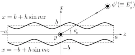
We consider the diffraction of an E-polarized plane wave by a finite parallel-plate waveguide with sinusoidal wall corrugation as shown in Figure 1, where the surface of the two planes is assumed to be finitely thin, perfectly electric conducting, and uniform in they-direction, being defined by

x=±b+hsinmz, |z| ≤a, (1)

where 2h is the corrugation amplitude and m(> 0) is the periodicity (surface roughness) parameter. Taking into account the geometry of the waveguide together with the fact that the electric field is parallel to they-axis, this scattering problem is reduced to a two-dimensional problem.

Let us define the total electric fieldφt(x, z) [≡Eyt(x, z)] by

φt(x, z) =φi(x, z) +φ(x, z), (2) whereφi(x, z) is the incident field ofE polarization given by

φi(x, z) =e−ik(xsinθ0+zcosθ0)_{, 0< θ}

0< π/2 (3)

with k[≡ω(ε0μ0)1/2] being the free-space wavenumber. The scattered field φ(x, z) satisfies the

two-dimensional Helmholtz equation

Figure 1. Geometry of the problem.

Nonzero components of the scattered electromagnetic fields are derived from the following relation:

(Ey, Hx, Hz) =

φ, i ωμ0

∂φ ∂z,

1 iωμ0

∂φ ∂x

. (5)

The total electric field φt satisfies the perfect conductor condition

φt(±b+hsinmz, z) = 0, |z|< a (6) on the waveguide walls. We assume that the corrugation amplitude 2h is small compared with the wavelength and expand Eq. (6) in terms of the Taylor series. Then by ignoring the O(h2_{) terms from}

the Taylor expansion, we obtain that

φt(±b, z) +hsinmz∂φ

t_{(±b, z)}

∂z +O(h

2_{) = 0, |z|< a. (7)}

Equation (7) is the approximate boundary condition used throughout the remaining part of this paper. We note that, by letting h →0 in Eq. (7), the problem reduces to the diffraction problem involving a flat, finite parallel-plate waveguide.

For convenience of analysis, we assume that the medium is slightly lossy as in k= k1+ik2 with

0 < k2 k1. The solution for real k is obtained by letting k2 → +0 at the end of analysis. In view

of the radiation condition, it follows that the scattered fieldφ(x, z) behaves like the diffracted field for fixed xas|z| → ∞. Hence we can show that

φ(x, z)∼CH0(1)(kρ)∼Cρ−1/2eik1ρe−k2ρ=O

e−k2|z|

=O

e−k2|z|cosθ0

(8)

as |z| → ∞, where ρ = (x2+z2)1/2, and C and C are constants. In Eq. (8), H0(1)(·) is the Hankel

function of the first kind.

We introduce the Fourier transform of the scattered fieldφ(x, z) as

Φ(x, α) = (2π)−1/2

_∞

−∞φ(x, z)e

iαz_{dz, (9)}

where α = Reα+iImα(≡ σ+iτ). In view of Eq. (8), it follows that Φ(x, α) is regular in the strip |τ|< k2cosθ0 of the complex α-plane. We also introduce the Fourier integrals as in

Φ_±(x, α) = ±(2π)−1/2

_±∞

±a φ(x, z)e iα(z∓a)

dz, (10)

Φ1(x, α) = (2π)−1/2

_a

−aφ(x, z)e

iαz_{dz, (11)}

Then it is seen that Φ(_±n)(x, α) are regular in τ ≷∓k2cosθ0 whereas Φ1(x, α) is an entire function. It

follows from Eqs. (9)–(11) that

Φ(x, α) =e−iαaΦ₋(x, α) + Φ1(x, α) +eiαaΦ+(x, α). (12)

Taking the Fourier transform of Eq. (4) and making use of Eq. (8), we derive that

whereγ(α) = (α2−k2)1/2. Sinceγ(α) is a double-valued function ofα, we choose its proper branch so thatγ(α) reduces to−ik whenα= 0. The solution of Eq. (13) is expressed as

Φ(x, α) = A(α)e−γ(α)x, x > b,

= B(α)e−γ(α)x+C(α)eγ(α)x, |x|< b,

= D(α)eγ(α)x, x <−b, (14)

where A(α),B(α), C(α), and D(α) are unknown functions. For convenience of analysis, we introduce the Fourier integrals as in

P±(α) = ±(2π)−1/2

_±∞

±a

φ(b+ 0, z) +hsinmz∂φ(b+ 0, z) ∂x

eiα(z∓a)dz, (15)

Q±(α) = ±(2π)−1/2

_±∞

±a

φ(−b−0, z) +hsinmz∂φ(−b−0, z) ∂x

eiα(z∓a)dz, (16)

M1(α)

N1(α)

= (2π)−1/2

a

−a

∂φ(±b+ 0, z)

∂x −

∂φ(±b−0, z) ∂x

eiαzdz, (17)

F1,2(α) = (2π)−1/2

_a

−a

φ(±b, z) +hsinmz∂φ(±b, z) ∂x

eiαzdz. (18)

Taking into account the approximate boundary condition on the waveguide surface as given by Eq. (7) and carrying out some manipulations, we find from Eqs. (10), (11), and (12) that

P+(α) +P−(α) +F1(α) = Φ (b+ 0, α) + h

2i Φ

_{(b+ 0, α+m)−Φ(b+ 0, α−m), (19)}

Q+(α) +Q−(α) +F2(α) = Φ (−b−0, α) + h

2i Φ

_{(−b−0, α+m)−Φ(−b−0, α−m), (20)}

where the prime denotes differentiation with respect tox. Substituting the scattered field expression in Eq. (14) into Eqs. (19), (20), and (17), it follows that

P+(α) +P−(α) +F1(α) = A(α)e−γ(α)b +ih

2

γ(α+m)A(α+m)e−γ(α+m)b

−γ(α−m)A(α−m)e−γ(α−m)b

, (21)

Q+(α) +Q−(α) +F2(α) = D(α)e−γ(α)b −ih

2

γ(α+m)D(α+m)e−γ(α+m)b

−γ(α−m)D(α−m)e−γ(α−m)b

, (22)

M1(α) = −γ(α)

A(α)e−γ(α)x−B(α)e−γ(α)x+C(α)eγ(α)x

, (23)

N1(α) = −γ(α)

B(α)eγ(α)x−C(α)e−γ(α)x+D(α)e−γ(α)x

, (24)

Φ(b+ 0, α)−Φ(b−0, α) = γ2(α)

[A(α)−B(α)]e−r(α)b−C(α)er(α)b

, (25)

Φ(−b+ 0, α)−Φ(−b−0, α) = B(α)er(α)b + [C(α)−D(α)]e−r(α)b, (26)

where the prime denotes differentiation with respect to x. Making use of the continuity of tangential electric fields across x=±band Eq. (2), we deduce the following relations:

Φ(−b+ 0, α)−Φ(−b−0, α) = (2π)−1/2ih

2 [N1(α+m)−N1(α−m)], (27)

Φ(b+ 0, α)−Φ(b−0, α) = (2π)−1/2ih

Substituting Eqs. (25) and (26) into Eqs. (28) and (27) respectively, we can derive equations which relate A(α), B(α), C(α), and D(α) with M1(α) and N1(α). Solving these equations for A(α), B(α),

C(α), andD(α), we find that

A(α) = −e −γ(α)b

2

N1(α)

γ(α) −(2π) −1/2ih

2 [N1(α+m)−N1(α−m)]

−e−γ(α)b 2

M1(α)

γ(α) −(2π) −1/2ih

2 [M1(α+m)−M1(α−m)]

, (29)

B(α) = −e −γ(α)b

2

N1(α)

γ(α) −(2π) −1/2ih

2 [N1(α+m)−N1(α−m)]

, (30)

C(α) = −e −γ(α)b

2

M1(α)

γ(α) + (2π) −1/2ih

2 [M1(α+m)−M1(α−m)]

, (31)

D(α) = −e −γ(α)b

2

M1(α)

γ(α) + (2π) −1/2ih

2 [M1(α+m)−M1(α−m)]

−eγ(α)b 2

N1(α)

γ(α) + (2π) −1/2ih

2 [N1(α+m)−N1(α−m)]

. (32)

Substituting Eqs. (29) and (32) into Eqs. (21) and (22), respectively and using the boundary conditions, we arrive at

S(α) +G1(α) = −K(α)U1(α) +ih

4 e

−2γ(α+m)b_−(2π)−1/2

e−2γ(α)b+ (2π)−1/2−1

V−(α+m)

+

(2π)−1/2e−2γ(α)b−e−2γ(α−m)b−(2π)−1/2+ 1

V−(α−m)

, (33)

D(α) +G2(α) = −L(α)V1(α) + ih

4 (2π)

−1/2_e−2γ(α)b _−e−2γ(α+m)b_{+ (2π)}−1/2 _−1U

−(α+m)

+

e−2γ(α−m)b−(2π)−1/2e−2γ(α)b−(2π)−1/2+ 1

U−(α−m)

, (34)

where

S(α) = [P+(α) +P−(α)] + [Q+(α) +Q−(α)], (35)

D(α) = [P+(α) +P−(α)]−[Q+(α) +Q−(α)], (36)

U1(α) = M1(α) +N1(α), V1(α) =M1(α)−N1(α), (37)

G1,2(α) = F1(α)±F2(α) =e−ikbsinθ0

e−iαaA0−eiαaB0

α−kcosθ0

+ikhsinθ0 2

2

n=1

(−1)n+1e −iαa_A

n−eiαaBn α−kcosθn

±eikbsinθ0

e−iαaA0−eiαaB0

α−kcosθ0

+ikhsinθ0 2

2

n=1

(−1)n+1e −iαa_A

n−eiαaBn α−kcosθn

, (38)

A0 = −(2π)−1/2ieikacosθ0, B0=−(2π)−1/2ie−ikacosθ0, (39)

An = (2π)−1/2eikacosθn, Bn= (2π)−1/2e−ikacosθn (40)

cosθ1,2 = cosθ0∓m/k, (41)

K(α) = e

−γ(α)b_coshγ(α)b

γ(α) , L(α) =

e−γ(α)bsinhγ(α)b

γ(α) . (42)

Equations (33) and (34) are the simultaneous Wiener-Hopf equations satisfied by S(α), D(α), U1(α),

and V1(α), which hold for anyα in the strip |τ|< k2cosθ0. In the above, K(α) and L(α) defined by

3. ZERO- AND FIRST-ORDER WIENER-HOPF EQUATIONS

In order to solve the Wiener-Hopf Equations (33) and (34), we express the unknown functions S(α), D(α),U1(α), and V1(α) in terms of perturbation series expansions in h omittingO(h2) as

S(α) = S0(α) +hS1(α) +O(h2), (43) D(α) = D0(α) +hD1(α) +O(h2), (44)

U1(α) = U1(0)(α) +hU (1)

1 (α) +O(h2), (45)

V1(α) = V (0)

1 (α) +hV (1)

1 (α) +O(h 2₎

. (46)

We can also express the known functions G1(α) and G2(α) defined by Eq. (38) in the form of a

perturbation series in h as in

G1(α) = G01(α) +hG11(α) +O(h2), (47)

G2(α) = G02(α) +hG12(α) +O(h2). (48)

In view of Eqs. (35) and (36), S0(α) and S1(α) in Eq. (43) and D0(α) and D1(α) in Eq. (44) can be expressed as follows:

S0(α) = eiαaS+0(α) +e−iαaS−0(α) =eiαa P+0(α) +Q0+(α)

+e−iαa P₋0(α) +Q0₋(α), (49)

S1(α) = eiαaS+1(α) +e−iαaS−1(α) =eiαa P+1(α) +Q1+(α)

+e−iαa P₋1(α) +Q1₋(α), (50)

D0(α) = eiαaD+0(α) +e−iαaD0−(α) =eiαa P+0(α)−Q0+(α)

+e−iαa P₋0(α)−Q0₋(α), (51)

D1(α) = eiαaD+1(α) +e−iαaD1−(α) =eiαa P+1(α)−Q1+(α)

+e−iαa P₋1(α)−Q1₋(α). (52) We substitute Eqs. (43)–(48) into Eqs. (33) and (34), and make use of Eqs. (49)–(52) in the resultant equations. After ignoring the O(h2) terms, the original Wiener-Hopf equations can be separated into theO(1) equations

K(α)U1(0)(α) +eiαaS˜ 0

(+)(α) +e−iαaS˜ 0

−(α) = 0, (53)

L(α)V1(0)(α) +eiαaD˜ 0

(+)(α) +e−iαaD˜ 0

−(α) = 0 (54)

and theO(h) equations

K(α)U1(1)(α) +eiαaS˜ 1

(+)(α) +e−iαaS˜ 1

−(α)−₄i e−2γ(α+m)b−(2π)−1/2e−2γ(α)b+ (2π)−1/2 −1

V1(0)(α+m) +

(2π)−1/2e−2γ(α)b−e−2γ(α−m)b−(2π)−1/2+ 1

V1(0)(α−m)

= 0, (55)

L(α)V1(1)(α) +eiαaD˜(+)1 (α) +e−iαaD˜−1(α)−

i

4 (2π) −1/2

e−2γ(α)b−e−2γ(α+m)b+ (2π)−1/2−1

U1(0)(α+m) +

e−2γ(α−m)b−(2π)−1/2e−2γ(α)b −(2π)−1/2+ 1

U1(0)(α−m)

= 0 (56)

for|τ|< k2cosθ0, where

˜

S(+)0 (α) = P 0

+(α) +Q0+(α)−2B0

cos(kbsinθ0)

α−kcosθ0 ,

(57)

˜

S₋0(α) = P₋0(α) +Q0₋(α) + 2A0

cos(kbsinθ0)

α−kcosθ0 ,

(58)

˜

D(+)0 (α) = P 0

+(α)−Q0+(α) + 2iB0

sin(kbsinθ0)

α−kcosθ0 ,

(59)

˜

D₋0(α) = P₋0(α)−Q0₋(α)−2iA0

sin(kbsinθ0)

α−kcosθ0 ,

(60)

˜

S(+)1 (α) = P 1

+(α) +Q1+(α) + 2

n=1

(−1)nBn(C1+C2) α−kcosθn ,

˜

S₋1(α) = P₋1(α) +Q1₋(α)−

2

n=1

(−1)nAn(C1+C2) α−kcosθn ,

(62)

˜

D1(+)(α) = P+1(α)−Q1+(α) + 2

n=1

(−1)nBn(C1−C2) α−kcosθn ,

(63)

˜

D1₋(α) = P₋1(α)−Q1₋(α)−

2

n=1

(−1)nAn(C1−C2) α−kcosθn ,

(64)

Cn = ik sinθ0

2 e

±ikbsinθ0 ₍₆₅₎

forn= 1,2.

Equations (53), (54) and (55), (56) are the zero- and first-order Wiener-Hopf equations, respectively. The zero-order problem corresponds to the diffraction by a flat, finite parallel-plate waveguide, whereas the first-order problem is important since it contains the effect due to the sinusoidal corrugation.

4. EXACT AND ASYMPTOTIC SOLUTIONS

The kernel functionK(α) and L(α) defined by Eq. (42) are factorized as in [15–18]

K(α) = K+(α)K−(α) =K+(α)K+(−α), (66)

L(α) = L+(α)L−(α) =L+(α)L+(−α), (67)

where

K+(α) = (coskb)1/2eiπ/4(k+α)−1/2exp

iγ(α)b π ln

α−γ(α) k

·exp

iαb π

1−C+ ln π 2kb +i

π 2

∞

n=1,odd

1 + α iγn

e2iαb/nπ, (68)

L+(α) =

sinkb k

1/2

exp

iγ(α)b π ln

α−γ(α) k

·exp

iαb π

1−C+ ln2π kb +i

π 2

∞

n=2,even

1 + α iγn

e2iαb/nπ (69)

withC(= 0.57721566. . .) being Euler’s constant and

γn= (nπ/2b)2−k2

1/2

. (70)

It seems from Eqs. (66) and (67) thatK±(α) and L±(α) are regular and nonzero in τ ≷∓k2. We can

also verify that

K±(α)∼(∓2iα)−1/2, L±(α)∼(∓2iα)−1/2 (71) asα→ ∞ withτ ≷∓k2. We shall now solve the zero-order Wiener-Hopf Equations (53), (54) and the

first-order Wiener-Hopf Equations (55), (56) to derive the exact and asymptotic solutions.

4.1. Solution of the Zero-Order Wiener-Hopf Equations (53) and (54)

at the exact solution with the result that

˜

S(+)0 (α) = −K+(α)

2B0cos(kbsinθ0)

K+(kcosθ0)(α−kcosθ0)

+1 2

σsu0(α)−σud0(α)

−1 2

us0(α)−ud0(α) = 0, (72)

˜

S₋0(α) = −K−(α)

− 2A0cos(kbsinθ0)

K−(kcosθ0)(α−kcosθ0)

+1 2

σsu0(−α)−σdu0(−α)

−1 2

us0(−α)−ud0(−α) = 0, (73)

˜

D(+)0 (α) = −L+(α)

− 2iA0sin(kbsinθ0)

L+(kcosθ0)(α−kcosθ0)

+ 1 2

σ_vs0(α)−σdv0(α)

−1 2

v0s(α)−v0d(α) = 0, (74)

˜

D₋0(α) = −L−(α)

2iA0sin(kbsinθ0)

L−(kcosθ0)(α−kcosθ0)

+ 1 2

σvs0(−α) +σvd0(−α)

−1 2

v0s(−α) +v0d(−α) = 0, (75)

where

us,d0 (α) =

1 πi

_k+i∞

k

e2iβaγ(β)K+(β) ˜S₍₊₎s0,d0(β)

β+α dβ, (76)

vs,d0 (α) =

1 πi

_k+i∞

k

e2iβaγ(β)L+(β) ˜Ds₍₊₎0,d0(β)

β+α dβ, (77)

σs,du (α) = ∞ n=1 odd _nπ 2b

2 K+(iγn)e−2aγnS˜₍₊₎s0,d0(iγn) ibγn(α+iγn) ,

(78)

σs,dv (α) = ∞ n=2 even _nπ 2b

2 L+(iγn)e−2aγnD˜s₍₊₎0,d0(iγn) ibγn(α+iγn)

(79)

Introducing the functions ˜

S₍₊₎s0,d0(α) = ˜S(+)0 (α)±S˜ 0

−(−α), D˜(+)s0,d0(α) = ˜D 0

(+)(α)±D˜ 0

−(−α), (80)

Equations (72)–(75) can be rearranged as

˜

S₍₊₎s0,d0(α)

b =b

−1/2_K +(α)

±b−1/2us,d0 (α)∓

∞

n=2

anpnsso,dn 0 b(α+iγ2n−3) ∓

Au0

b(α+kcosθ0)−

B0u

b(α−kcosθ0)

,(81)

˜

Ds₍₊₎0,d0(α)

b =b

−1/2

L+(α)

±b−1/2vs,d0 (α)∓

∞

n=2

˜

anp˜ndso,dn 0 b(α+iγ2n−2) ±

Av0

b(α+kcosθ0)

+ B

v

0

b(α−kcosθ0)

,(82)

where

a01 = kb, ˜a01=kb, (83)

a0n =

(2n−3)2π2e−2aγ2n−3 4biγ2n−3 ,

˜ a0n =

(2n−2)2π2e−2aγ2n−2

4biγ2n−2 , n≥

2, (84)

p01 = b−1/2K+(k), p˜01 =b−1/2L+(k), (85)

ss0,d0 = b−1S˜₍₊₎s0,d0(k), ds0,d0 =b−1D˜₍₊₎s0,d0(k), (87)

ssn0,d0 = b−1S˜s

0,d0

(+) (iγ2n−3), d

s0,d0

n =b−1D˜s

0,d0

(+) (iγ2n−2), n≥2. (88)

Equations (81) and (82) are formal since they contain the branch-cut integrals with unknown integrands and the infinite series with unknown coefficients. Therefore it is necessary to develop approximation procedures for obtaining explicit approximate solutions for numerical computation.

Regarding the branch-cut integralsus,d0 (α) andv

s,d

0 (α) with the unknown integrands ˜S

s0,d0

(+) (β) and

˜

Ds₍₊₎0,d0(β), we apply the rigorous asymptotic method developed by Kobayashi [37]. Omitting the details, we obtain a high-frequency expressions ofus,d0 (α) and v0s,d(α) for large k|a|as in

u0s,d(α) ∼kK+(k) ˜S₍₊₎s0,d0(k)ξ(α), v0s,d(α)∼kL+(k) ˜D₍₊₎s0,d0(k)ξ(α), (89)

where

ξ(α) =−2a

1/2_e2ika

π Γ1[1/2,−2i(α+k)a]. (90) In Eq. (90), Γ1(·,·) is the generalized gamma function introduced by Kobayashi [38] and is defined by

Γm(u, v) =

_∞

0

tu−1e−t

(t+v)mdt (91)

for Reu >0,|v|>0,|argv|< π, and positive integer m.

We next evaluate the infinite series σus,d(α) and σs,dv (α) with the unknown coefficients ssn0,d0 and dsn0,d0. Taking into account the edge condition, we can show that ˜S₍₊₎s0,d0(α) and ˜Ds₍₊₎0,d0(α) have the asymptotic behavior

˜

S₍₊₎s0,d0(α), D˜₍₊₎s0,d0(α) =O(α−3/2), α→ ∞. (92) Therefore, the infinite series contained in Eqs. (81) and (82) are approximated with the choice of a large positive integer N by

∞

n=2

anpnssn b(α+iγ2n−3) ≈

N

n=2

anpnssn b(α+iγ2n−3)

+Ku(1)S

(1)

uN(α), (93)

∞

n=2

˜ anp˜ndsn b(α+iγ2n−2) ≈

N

n=2

˜ anp˜ndsn b(α+iγ2n−2)

+Kv(1)S

(1)

vN(α), (94)

whereKu(1) and Kv(1) are unknown constants independent ofn, and

S_uN(1)(α) = ∞

n=N+1

an(bγ2n−3)−2

b(α+iγ2n−3),

(95)

S_vN(1)(α) = ∞

n=N+1

an(bγ2n−2)−2

b(α+iγ2n−2).

(96)

By substituting Eqs. (89), (93), and (94) into Eqs. (81) and (82), we arrive at the explicit approximate solutions of the Wiener-Hopf Equations (53) and (54) with the result that

˜

S₍₊₎s0,d0(α)

b ≈ b

−1/2

K+(α)

±a01p01ss0,d0ξ(α)∓

N

n=2

anpnsso,dn 0 b(α+iγ2n−3)

∓Ku(1)S

(1)

uN(α)∓

Au0

b(α+kcosθ0)−

B0u

b(α−kcosθ0)

, (97)

˜

D₍₊₎s0,d0(α)

b ≈ b

−1/2

L+(α)

±˜a01p˜01ds0,d0ξ(α)∓

N

n=2

˜

anp˜ndso,dn 0 b(α+iγ2n−2)

∓Kv(1)S

(1)

vN(α)±

Av0

b(α+kcosθ0)

+ B

v

0

b(α−kcosθ0)

4.2. Solution of the First-Order Wiener-Hopf Equations (55) and (56)

Multiplying both sides of Eq. (55) bye±iαa/K∓(α), Eq. (56) bye±iαa/L∓(α) respectively, and applying the decomposition procedure, we arrive at the exact solution with the result that

˜

S₍₊₎s1,d1(α) K+(α)

+

2

n=1

(−1)n+1

Bn(C1+C2)

K+(kcosθn)(α−kcosθn) ±

e2ikacosθn_B

n(C1+C2)

K−(kcosθn)(α+kcosθn)

+σs,du1(α)−us,d1 (α)

−Ts1,d1(α)

K+(α)

= 0, (99)

˜

Ds₍₊₎1,d1(α) L+(α)

+

2

n=1

(−1)n+1

Bn(C1−C2)

L+(kcosθn)(α−kcosθn)±

e2ikacosθn_B

n(C1−C2)

L−(kcosθn)(α+kcosθn)

+σs,d_v1(α)−v

s,d

1 (α)

−Qs1,d1(α)

L+(α)

= 0, (100)

where

Ts1,d1(α) = ie−iαa/4 e−2γ(α−m)b+C3(α)

V1(0)(α−m)∓V (0)

1 (−α−m)

+

e−2γ(α+m)b+C3(α) V₁(0)(α+m)∓V₁(0)(−α−m) , (101)

Qs1,d1(α) = ie−iαa/4 e−2γ(α−m)b+C4(α) U (0)

1 (α−m)∓U (0)

1 (−α+m)

−e−2γ(α+m)b+C4(α) U1(0)(α+m)∓U (0)

1 (−α−m) , (102)

C3,4(α) = −(2π)−1/2

e−2γ(α)b∓1

∓1, (103)

us,d1 (α) =

1 πi

_k+i∞

k

e2iuaγ(u)K+(u) ˜S₍₊₎s1,d1(u)

u+α du, (104)

vs,d1 (α) =

1 πi

_k+i∞

k

e2iuaγ(u)L+(u) ˜D₍₊₎s1,d1(u)

u+α du, (105)

σs,du1(α) =

∞ n=1 odd _nπ 2b

2K+(iγn)e−2aγnS˜(+)s1,d1(iγn)

ibγn(α+iγn) ,

(106)

σs,d_v1(α) =

∞ n=2 even _nπ 2b

2L+(iγn)e−2aγnD˜₍₊₎s1,d1(iγn) ibγn(α+iγn)

(107)

with

˜

S₍₊₎s1,d1(α) = ˜S(+)1 (α)±S˜ 1

−(−α), D˜(+)s1,d1(α) = ˜D 1

(+)(α)±D˜ 1

−(−α). (108)

In order to derive approximate solutions for numerical computation, it is required to evaluate the unknown functions us,d1 (α) and v

s,d

1 (α) defined by Eqs. (104) and (105) as well as σ

s,d

u1(α) and σ

s,d v1(α)

defined by Eqs. (106) and (107). To this end, we may apply a procedure similar to that employed for the zero-order Wiener-Hopf equations. Omitting the whole details, we arrive at the approximate solutions as in

˜

S(+)s1·d1(α)≈

K+(α)

b1/2

±a11p11ss1,d1ξ(α)∓

N−1

n=2

a1np1nss

1,d1

n

b(α+iγ2n−3) ±K (2)

u S

(2)

+b1/2

2

n=1

(−1)n

Bn(C1+C2)

K+(kcosθn)(α−kcosθn)±

e2ikacosθn_B

n(C1+C2)

K−(kcosθn)(α+kcosθn)

+Ts1,d1(α),

(109)

˜

Ds(+)1·d1(α)≈

L+(α)

b1/2

±˜a11p˜11ds1,d1ξ(α)∓

N−1

n=2

˜ a1np˜1nds

1,d1

n

b(α+iγ2n−2) ∓K (2)

v S

(2)

vN(α)

+b1/2

2

n=1

(−1)n

Bn(C1−C2)

L+(kcosθn)(α−kcosθn) ±

e2ikacosθn_B

n(C1−C2)

L−(kcosθn)(α+kcosθn)

+Qs1,d1(α),

(110)

where

a11 =kb, ˜a11 =kb, (111)

a1n =

(2n−3)2_π2_e−2aγ2n−3 4biγ2n−3 ,

˜ a1n=

(2n−2)2_π2_e−2aγ2n−2

4biγ2n−2 , n≥

2, (112)

p11 =b−1/2K+(k), p˜11=b−1/2L+(k), (113)

p1n =b−1/2K+(iγ2n−3), p˜n1 =b−1/2L+(iγ2n−2), n≥2, (114)

ss1,d1 = ˜S₍₊₎s1,d1(k), ds1,d1 = ˜Ds₍₊₎1,d1(k), (115)

ssn1,d1 = ˜S s1,d1

(+) (iγ2n−3), d

s1,d1

n = ˜D s1,d1

(+) (iγ2n−2), n≥2. (116)

S_uN(2)(α) = ∞

n=N+1

an(bγ2n−3)−2

b(α+iγ2n−3),

(117)

S_vN(2)(α) = ∞

n=N+1

an(bγ2n−2)−2

b(α+iγ2n−2),

(118)

u_s,d1 (α) ∼kK+(k) ˜S₍₊₎s1,d1(k)ξ(α), (119)

vs,d1 (α) ∼kL+(k) ˜D₍₊₎s1,d1(k)ξ(α) (120)

aska→ ∞.

4.3. Determination of the Unknown Coefficients

Equations (97), (98), (109), and (110) are approximate solutions to the simultaneous Wiener-Hopf Equations (53)–(56), and hold uniformly in θ0 for large N and |k|a, where the unknownssns1,d1, ssn0,d0, dns0,d0, and dns1,d1 forn= 1,2,3, . . . , N as well asKu(1),Kv(1),Ku(2), and Kv(2) are contained.

In order to determine these unknowns, we set α=k, iγ2m−3 form= 2,3,4, . . . , N+ 1 in Eqs. (97)

and (109). We also setα=k, iγ2m−2 form= 2,3,4, . . . , N+ 1 in Eqs. (98) and (110). These procedures

lead to the two sets of (N+1)×(N+1) equations, wheress_N1+1,d1 andd

s1,d1

N+1 are involved. SinceN is a large

positive number, we can employ Eq. (92) to replace ss_N1,d₊₁1 and ds_N1₊₁,d1 by their asymptotic expressions

5. SCATTERED FAR FIELD

In this section, we shall derive an asymptotic expression of the field outside the waveguide. The region outside the waveguide actually includes |z| > a with |x| < b, but contributions from this region are negligibly small at large distance from the origin. Therefore, only the scattered far field for|x|> b will be discussed in the following. The scattered fieldφ(x, z) in the real space can be derived by taking the inverse Fourier transform of Eq. (9) according to the formula

φ(x, z) = (2π)−1/2

_∞+ic

−∞+ic

Φ(x, α)e−iαzdα, (121)

wherec is a constant satisfying|c|< k2cosθ0.

Substituting Eq. (37) into Eqs. (45) and (46), we obtain that

M1(α)

N1(α)

= 1 2

U1(0)(α)±V (0) 1 (α)

+h

U1(1)(α)±V (1) 1 (α)

. (122)

Furthermore substituting Eq. (122) into Eqs. (29) and (32) and taking into account Eqs. (14) and (121), we arrive at an integral representation for the scattered field with the result that

φ(x, z) =φ(0)(x, z) +hφ(1)(x, z), (123) where

φ(0)(±b, z) = −(2π)−1/2

_∞+ic

−∞+ic 1 2γ(α)

U1(0)(α) coshγ(α)b

±V1(0)sinhγ(α)b

e∓γ(α)x−iαzdα, x≷b, (124)

φ(1)(±b, z) = (2π)−1/2

_∞+ic

−∞+ic

− h

2γ(α) U

(1)

1 (α) coshγ(α)b±V (1)

1 (α) sinhγ(α)b

±(2π)−1/2ih

4 U

(0)

1 (α+m)−U (0)

1 (α−m)

coshγ(α)b

±V1(0)(α+m)−V (0)

1 (α−m)

sinhγ(α)b

e∓γ(α)x−iαzdα, x≷±b. (125)

As seen above, Eqs. (124) and (125) are the and first-order scattered fields, respectively. The zero-order scattered field corresponds to the problem of diffraction by a flat, finite parallel-plate waveguide. In the following, we shall derive asymptotic expressions of the zero- and first-order scattered far fields explicitly.

Since the integrand of Eq. (124) has branch points at α = ±k, evaluation in closed form is in general difficult. However, we may apply the saddle point method to derive an asymptotic expression at large distances from the origin. Introduce the cylindrical coordinates (ρ, θ) centered at the origin as follows:

x=ρsinθ, z=ρcosθ, for −π < θ < π. (126) By means of the saddle point method, we can derive a far field asymptotic expression of the scattered field with the result that

φ(0)(ρ, θ)∼ − 1 2γ(−kcosθ)

U1(0)(−kcosθ) coshγ(−kcosθ)b

±V1(0)(−kcosθ) sinhγ(−kcosθ)b

ksin|θ|e

i(kρ−π/4)

(kρ)1/2 (127)

forx≷±bas kρ→ ∞.

Next we shall derive an asymptotic expression of the first-order scattered field φ(1)(x, z). In view of Eq. (125), the first-order scattered field can be written as

where

φ(1)u (x, z) = −(2π)−1/2

_∞+ic

−∞+ic 1 2γ(α)h

U1(1)(α) coshγ(α)b

±V1(1)(α) sinhγ(α)b

e∓γ(α)x−iαzdα, x≷±b, (129)

φ(1)v (x, z) = ±(2π)−1/2·

_∞+ic

−∞+ic ih

4 U

(0)

1 (α+m)−U (0)

1 (α−m)

coshγ(α)b

±V1(0)(α+m)−V (0)

1 (α−m)

sinhγ(α)b

e∓γ(α)x−iαzdα, x≷±b. (130)

Applying the saddle point method with the aid of the cylindrical coordinate defined by Eq. (126), it is found thatφ(1)u (x, z) has the asymptotic expression

φ(1)_u (ρ, θ)∼ − 1 2γ(−kcosθ)

U1(1)(−kcosθ) coshγ(−kcosθ)b

±V1(1)(−kcosθ) sinhγ(−kcosθ)b

ksin|θ|e

i(kρ−π/4)

(kρ)1/2 (131)

forx≷±bas kρ→ ∞.

An asymptotic evaluation ofφ(1)v (x, z) defined by Eq. (130) is in general difficult, since the integrand has branch points at α =±k+m,±k−m as well as α =±k. For simplicity, we assume |m/k| 1, which implies that the period of corrugation is large compared with the wavelength. Then in the process of asymptotic evaluation, we can ignore contributions from branch-cut integrals occurring due to the branch points at α=±k+m,±k−m. Therefore the simple saddle point method may be employed to obtain a far field expression with the result that

φ(1)v (ρ, θ)∼ ∓ i

4 U

0

1(−kcosθ(1))−U10(−kcosθ(2))

coshγ(−kcosθ)b

±V10(−kcosθ(1))−V10(−kcosθ(2))

sinhγ(−kcosθ)b

ksin|θ|e

i(kρ−π/4)

(kρ)1/2 (132)

forx≷±bas kρ→ ∞. where

θ(1) = cos−1(cosθ−m/k), θ(2)= cos−1(cosθ+m/k). (133) As seen above, substitution of Eqs. (131) and (132) into Eq. (128) yields an explicit far field expression of the first-order scattered far field, and holds for arbitrary incidence and observation angles.

6. NUMERICAL RESULTS AND DISCUSSION

In this section, we shall present numerical examples of the RCS and discuss far field scattering characteristics of the waveguide in detail. Since this is a two-dimensional problem, the RCS per unit length is given by

ρ= lim ρ→∞

2πρ|φ|2/|φi|2, (134)

where

other hand, in order to validate the far field asymptotic expression ofφ(1)v (x, z) given by Eq. (132), the ratiom/k has been taken asm/k≤0.2 in numerical computations. Under this condition, contributions from branch-cut integrals due to the branch points atα=±k+mand±k−marising in the process of asymptotic evaluation of Eq. (130) are small compared with the saddle point contribution and hence, Eq. (132) can be used with reasonable accuracy.

Figures 2–5 show numerical examples of the bistatic RCSσ/λas a function of observation angleθ

(a) (b)

-180 -120 -60 0 60 120 180

OBSERVATION ANGLE (DEG)

-180 -120 -60 0 60 120 180

OBSERVATION ANGLE (DEG) 0

40

20

-20

-40

BISTATIC RCS (dB)

0 40

20

-20

-40

BISTATIC RCS (dB)

corrugated waveguide flat waveguide

corrugated waveguide flat waveguide

Figure 2. Bistatic RCS σ/λ[dB] of a flat waveguide and a corrugated waveguide for θ0= 60◦,N = 1,

2a= 10λ, m/k= 0.1, 2b= 4λ. (a) 2h= 0.02λ. (b) 2h= 0.1λ.

(a) (b)

-180 -120 -60 0 60 120 180

OBSERVATION ANGLE (DEG)

-180 -120 -60 0 60 120 180

OBSERVATION ANGLE (DEG) 0

40

20

-20

-40

BISTATIC RCS (dB)

0 40

20

-20

-40

BISTATIC RCS (dB)

corrugated waveguide flat waveguide

corrugated waveguide flat waveguide

Figure 3. Bistatic RCS σ/λ[dB] of a flat waveguide and a corrugated waveguide for θ0= 60◦,N = 5,

2a= 50λ, m/k= 0.1, 2b= 4λ. (a) 2h= 0.02λ. (b) 2h= 0.1λ.

(a) (b)

-180 -120 -60 0 60 120 180

OBSERVATION ANGLE (DEG)

-180 -120 -60 0 60 120 180

OBSERVATION ANGLE (DEG) 0

40

20

-20

-40

BISTATIC RCS (dB)

0 40

20

-20

-40

BISTATIC RCS (dB)

corrugated waveguide flat waveguide

corrugated waveguide flat waveguide

Figure 4. Bistatic RCS σ/λ[dB] of a flat waveguide and a corrugated waveguide for θ0= 60◦,N = 5,

for various values of N, 2a,m/k, and 2h, where the incidence angleθ0 and the waveguide width 2bare

fixed as 60◦ and 4λ, respectively. All these results provide comparisons on the scattering characteristics between the flat waveguide (black lines) and the corrugated waveguide (red lines). In the figures, the parameter m/k is important in numerical computation and is physically the periodicity (surface roughness) parameter. In addition,N(≡(2a/λ)(m/k)) implies the number of periods of the corrugation of the waveguide walls. The periodicity parameterm/k is chosen as 0.1 and 0.2 in Figures 2 and 3 and Figures 4 and 5, respectively. We have chosen the waveguide length and the corrugation depth as 2a= 10λ,25λ,45λ,50λ and 2h= 0.02λ,0.1λ, respectively.

It is seen from all the figures that the bistatic RCS has maximum peaks at θ=−120◦ and 120◦, which correspond to the incident and reflected shadow boundaries, respectively. Comparing the results for the corrugated waveguide with those for the flat waveguide, we observe that the effect of the sinusoidal corrugation of the waveguide walls is noticeable in the reflection region 90◦ < θ <180◦, and the bistatic RCS has sharp peaks at two particular observation angles around the specularly-reflected direction at θ=π−θ0(= 120◦). Consideration on the infinite periodic structure may offer physical understanding of

the scattering mechanism at these particular observation angles. Referring to (41), it is seen thatπ−θ1

andπ−θ2 are, respectively, propagation directions of the (−1) and (+1) order diffracted waves involved

in the Floquet mode arising in periodic structures of infinite extent [17]. The angles π−θ1, π−θ2 are,

respectively, 113.6◦,126.9◦ in Figures 2 and 3, and 107.5◦,134.4◦ in Figures 4 and 5, where somewhat large reflection is expected. In fact, we see that the observation angles associated with the two peaks aroundπ−θ0 are precisely coincident with the directions atπ−θ1 and π−θ2. On the other hand, the

peaks along the specular reflection π−θ0 is also expected from the grating theory since they exactly

correspond to the propagation direction of the zero-order Floquet mode. Therefore it is confirmed that

corrugated waveguide flat waveguide

corrugated waveguide flat waveguide

(a) (b)

-180 -120 -60 0 60 120 180

OBSERVATION ANGLE (DEG)

-180 -120 -60 0 60 120 180

OBSERVATION ANGLE (DEG) 0

40

20

-20

-40

BISTATIC RCS (dB)

0 40

20

-20

-40

BISTATIC RCS (dB)

Figure 5. Bistatic RCS σ/λ[dB] of a flat waveguide and a corrugated waveguide for θ0= 60◦,N = 9,

2a= 45λ, m/k= 0.2, 2b= 4λ. (a) 2h= 0.02λ. (b) 2h= 0.1λ.

(a) (b)

-180 -120 -60 0 60 120 180

OBSERVATION ANGLE (DEG)

-180 -120 -60 0 60 120 180

OBSERVATION ANGLE (DEG) 0

40

20

-20

-40

BISTATIC RCS (dB)

0 40

20

-20

-40

BISTATIC RCS (dB)

corrugated waveguide corrugated strip

corrugated waveguide corrugated strip

Figure 6. Bistatic RCSσ/λ[dB] of a corrugated strip and a corrugated waveguide forθ0 = 60◦,N = 1,

(a) (b)

-180 -120 -60 0 60 120 180

OBSERVATION ANGLE (DEG)

-180 -120 -60 0 60 120 180

OBSERVATION ANGLE (DEG) 0

40

20

-20

-40

BISTATIC RCS (dB)

0 40

20

-20

-40

BISTATIC RCS (dB)

corrugated waveguide corrugated strip

corrugated waveguide corrugated strip

Figure 7. Bistatic RCSσ/λ[dB] of a corrugated strip and a corrugated waveguide forθ0 = 60◦,N = 5,

2a= 25λ, m/k= 0.2, 2h= 0.1λ. (a) 2b= 2λ. (b) 2b= 6λ.

the three peaks at π−θ0, π−θ1, and π−θ2 in the results for the sinusoidal wall corrugation are due

to the periodicity of the sinusoidal surface of the waveguide.

It can also be observed by comparing Figures 2(a), 3(a), 4(a), and 5(a) with Figures 2(b), 3(b), 4(b), and 5(b) that the peaks occurring at the π−θ1 and π −θ2 directions become sharper with an

increase of 2h. On comparing Figure 2 for N = 1 with Figure 3 for N = 5, we see the peaks along π−θ1 and π−θ2 more clearly for larger N. This is because, if N increases, then the surface of the

waveguide walls approaches a periodic structure and hence, waves along the propagation directions of the particular Floquet modes are strongly excited.

We shall now investigate the scattering characteristics depending on the number of strips, namely a single corrugated strip and two corrugated strips (corrugated parallel-plate waveguide). Figures 6 and 7 show comparisons between these two structures. Scattering characteristics in the neighborhood of the main-lobe directions at θ = ±120◦ show close features for both cases as can be expected. The differences between a single strip and two strips occur noticeably for |θ|< 60◦ and 150◦ < θ < 180◦. This is because, in this region, the effect due to the radiation from waveguide modes becomes stronger.

7. CONCLUDING REMARKS

In this paper, we have analyzed the diffraction by a finite parallel-plate waveguide with sinusoidal wall corrugation using the Wiener-Hopf technique combined with the perturbation method. Assuming that the corrugation amplitude is small compared with the wavelength and expanding the scattered field in the form of a perturbation series, the problem has been reduced to the diffraction by a flat, finite parallel wall waveguide with a certain mixed boundary condition. Using this approximate boundary condition, the problem has been formulated in terms of the simultaneous Wiener-Hopf equations. The Wiener-Hopf equations have been solved via the factorization and decomposition procedure leading to the exact and approximate solutions. Taking the inverse Fourier transform and applying the saddle point method, an asymptotic expression of the scattered far field has been derived.

REFERENCES

1. Byelobrov, V. O., T. L. Zinenko, K. Kobayashi, and A. I. Nosich, “Periodicity matters: Grating or lattice resonances in the scattering by sparse arrays of subwavelength strips and wires,” IEEE Antennas Propagat. Mag., Vol. 57, No. 6, 34–45, 2015.

2. Shestopalov, V. P., The Riemann-Hilbert Method in the Theory of Diffraction and Propagation of Electromagnetic Waves, Kharkov University Press, Kharkov, 1971 (in Russian).

3. Nosich, A. I., “Green’s function-dual series approach in wave scattering by combined resonant scatterers,” Analytical and Numerical Methods in Electromagnetic Wave Theory, Chap. 9, M. Hashimoto, M. Idemen, and O. A. Tretyakov (eds.), Science House, Tokyo, 1993.

4. Shestopalov, V. P., L. N. Litvinenko, S. A. Masalov, and V. G. Sologub, Diffraction of Waves by Gratings, Kharkov University Press, Kharkov, 1973 (in Russian).

5. Shestopalov, V. P., A. A. Kirilenko, and S. A. Masalov, Convolution-type Matrix Equations in the Theory of Diffraction, Naukova Dumka Publishing, Kiev, 1984 (in Russian).

6. Nosich, A. I., “The method of analytical regularization in wave-scattering and eigenvalue problems: Foundations and review of solutions,”IEEE Antennas Propagat. Mag., Vol. 41, No. 3, 34–49, 1999. 7. Nosich, A. I., “Method of analytical regularization in computational photonics,”Radio Sci., Vol. 51,

1421–1430, 2016.

8. Ikuno, H. and K. Yasuura, “Improved point-matching method with application to scattering from a periodic surface,”IEEE Trans. Antennas Propagat., Vol. 21, No. 5, 657–662, 1973.

9. Okuno, Y., “The mode-matching method,”Analysis Methods for Electromagnetic Wave Problems, Chap. 4, E. Yamashita (ed.), Artech House, Boston, 1990.

10. Okuno, Y., “An introduction to the Yasuura method,” Analytical and Numerical Methods in Electromagnetic Wave Theory, Chap. 11, M. Hashimoto, M. Idemen, and O. A. Tretyakov (eds.), Science House, Tokyo, 1993.

11. Petit, R. (ed.), Electromagnetic Theory of Gratings, Springer-Verlag, Berlin, 1980.

12. Hinata, T. and T. Hosono, “On the scattering of electromagnetic wave by plane grating placed in homogeneous medium — Mathematical foundation of point-matching method and numerical analysis,”Trans. IECE Japan, Vol. J59-B, No. 12, 571–578, 1976 (in Japanese).

13. Yamasaki, T., K. Isono, and T. Hinata, “Analysis of electromagnetic fields in inhomogeneous media by Fourier series expansion methods — The case of a dielectric constant mixed a positive and negative regions,” IEICE Trans. Electron., Vol. E88-C, No. 12, 2216–2222, 2005.

14. Ozaki, R., T. Yamasaki, and T. Hinata, “Scattering of electromagnetic waves by multilayered inhomogeneous columnar dielectric gratings,”IEICE Trans. Electron., Vol. E90-C, No. 2, 295–303, 2007.

15. Noble, B., Methods Based on the Wiener-Hopf Technique for the Solution of Partial Differential Equations, Pergamon, London, 1958.

16. Weinstein, L. A., The Theory of Diffraction and the Factorization Method, The Golem Press, Boulder, 1969.

17. Mittra, R. and S.-W. Lee,Analytical Techniques in the Theory of Guided Waves, Macmillan, New York, 1971.

18. Kobayashi, K., “Wiener-Hopf and modified residue calculus techniques,” Analysis Methods for Electromagnetic Wave Problems, Chap. 8, E. Yamashita (ed.), Artech House, Boston, 1990. 19. Baldwin, G. L. and A. E. Heins, “On the diffraction of a plane wave by an infinite plane grating,”

Math. Scand., Vol. 2, 103–118, 1954.

20. Hills, N. L. and S. N. Karp, “Semi-infinite diffraction gratings — I,” Comm. Pure Appl. Math., Vol. 18, No. 1–2, 203–233, 1965.

21. L¨uneburg, E. and K. Westpfahl, “Diffraction of plane waves by an infinite strip grating,” Ann. Phys., Vol. 27, No. 3, 257–288, 1971.

M. Idemen, and O. A. Tretyakov (eds.), Science House, Tokyo, 1993.

23. Serbest, A. H., A. Kara, and E. L¨uneburg, “Scattering of plane waves at the junction of two corrugated half-planes,” Electromagnetics, Vol. 25, No. 1, 21–38, 2005.

24. Idemen, M. and A. Alkumru, “Diffraction of two-dimensional high-frequency electromagnetic waves by a locally perturbed two-part impedance plane,” Wave Motion, Vol. 42, 53–73, 2005.

25. Ayub, M., M. Ramzan, and A. B. Mann, “Acoustic diffraction by an oscillating strip,” Applied Mathematics and Computation, Vol. 214, 201–209, 2009.

26. Kobayashi, K., “Diffraction of a plane wave by the parallel plate grating with dielectric loading,” Trans. IECE Japan, Vol. J64-B, No. 10, 1091–1098, 1981 (in Japanese).

27. Kobayashi, K., “Diffraction of a plane electromagnetic wave by a parallel plate grating with dielectric loading: The case of transverse magnetic incidence,” Can. J. Phys., Vol. 63, No. 4, 453–465, 1985.

28. Kobayashi, K. and T. Inoue, “Diffraction of a plane wave by an inclined parallel plate grating,” IEEE Trans. Antennas Propagat., Vol. 36, No. 10, 1424–1434, 1988.

29. Kobayashi, K. and K. Miura, “Diffraction of a plane wave by a thick strip grating,” IEEE Trans. Antennas Propagat., Vol. 37, No. 4, 459–470, 1989.

30. Das Gupta, S. P., “Diffraction by a corrugated half-plane,” Proc. Vib. Prob., Vol. 3, No. 11, 413– 424, 1970.

31. Chakrabarti, A. and S. Dowerah, “Traveling waves in a parallel plate waveguide with periodic wall perturbations,”Can. J. Phys., Vol. 62, No. 3, 271–284, 1984.

32. Zheng, J. P. and K. Kobayashi, “Diffraction by a semi-infinite parallel-plate waveguide with sinusoidal wall corrugation: Combined perturbation and Wiener-Hopf analysis,” Progress In Electromagnetics Research B, Vol. 13, 75–110, 2009.

33. Zheng, J. P. and K. Kobayashi, “Combined Wiener-Hopf and perturbation analysis of the H -polarized plane wave diffraction by a semi-infinite parallel-plate waveguide with sinusoidal wall corrugation,” Progress In Electromagnetics Research B, Vol. 13, 203–236, 2009.

34. Kobayashi, K. and T. Eizawa, “Plane wave diffraction by a finite sinusoidal grating,”IEICE Trans., Vol. E74, No. 9, 2815–2826, 1991.

35. Eizawa, T. and K. Kobayashi, “Wiener-Hopf analysis of theH-polarized plane wave diffraction by a finite sinusoidal grating,” Progress In Electromagnetics Research, Vol. 149, 1–13, 2014.

36. Kobayashi, K., “Some diffraction problems involving modified Wiener-Hopf geometries,”Analytical and Numerical Methods in Electromagnetic Wave Theory, Chap. 4, M. Hashimoto, M. Idemen, and O. A. Tretyakov (eds.), Science House, Tokyo, 1993.

37. Kobayashi, K., “Solutions of wave scattering problems for a class of the modified Wiener-Hopf geometries,” IEEJ Transactions on Fundamentals and Materials, Vol. 133, No. 5, 233–241, 2013. 38. Kobayashi, K., “On generalized gamma functions occurring in diffraction theory,” J. Phys. Soc.