Connectivity in Semi-Algebraic Sets.

(1)

ABSTRACT

ROHAL, JAMES JOSEPH. Connectivity in Semi-Algebraic Sets. (Under the direction of Hoon Hong.)

(2)

(3)

Connectivity in Semi-Algebraic Sets

by

James Joseph Rohal

A dissertation submitted to the Graduate Faculty of North Carolina State University

in partial fulfillment of the requirements for the Degree of

Doctor of Philosophy

Applied Mathematics

Raleigh, North Carolina

2014

APPROVED BY:

Jonathan Hauenstein Mohab Safey El Din

Erich Kaltofen Agnes Szanto

Hoon Hong

(4)

DEDICATION

(5)

BIOGRAPHY

(6)

ACKNOWLEDGEMENTS

If you were to tell me eleven years ago that my academic career will culminate with me becoming an assistant professor, I would have told you that you were crazy. Yet, I somehow survived the entire ordeal. However, that would not have been possible without the help of my friends, family, and many professors along the way. You have all helped me maintain my sanity throughout this process and for that I wish to thank you from the bottom of my heart.

Let me begin with my friends. So many of you have pushed me to keep going when I faltered and helped provide the necessary distractions to live a normal life outside of academics. To Sofia, Jon, Scott, Stephen, Adam, Josh, and Ryan, you have all been my retreat; the people I go to when I need to be picked up. Without you, this thesis would not have been completed. To everyone else that I have met through the math department and over the course of my stay in North Carolina, you have made this past five years the most memorable of my life.

It goes without saying, my family members are the most amazing people in the world. There are no bigger cheerleaders than my parents. No finite number of words in this Acknowledgments section can begin to thank them for everything they have done for me. Without a doubt, they have been the most influential people in my life and have pushed me to achieve so much.

(7)

TABLE OF CONTENTS

LIST OF TABLES . . . vi

LIST OF FIGURES . . . vii

Chapter 1 Introduction . . . 1

1.1 Problem Statement . . . 5

1.2 Previous Work . . . 7

1.3 Algorithm . . . 8

1.3.1 Description of AlgorithmConnectivity . . . 9

1.3.2 Specification of SubalgorithmDestination . . . 16

1.4 Overview of Results . . . 17

1.4.1 Partial Correctness . . . 18

1.4.2 Termination . . . 21

1.4.3 Length Bound . . . 21

1.4.4 Experimental Results . . . 25

Chapter 2 Partial Correctness . . . 27

2.1 Preliminaries . . . 27

2.2 Proof of Main Result . . . 35

Chapter 3 Termination . . . 39

Chapter 4 Length Bound . . . 47

4.1.1 Bound on Trajectory Length in a Ball . . . 47

4.1.2 Ball Enclosing Connectivity Path . . . 53

Chapter 5 Experimental Results . . . 69

5.1 Non-Trivial Examples . . . 70

5.2 Computational Timings . . . 79

Chapter 6 Conclusion and Outlook . . . 84

(8)

LIST OF TABLES

Table 1.40 Approximate steepest ascent path lengths for a sample connectivity path connecting pand q. . . 23

Table 5.11 Abbreviations used throughout Section 5.2. . . 79

Table 5.12 Number of instances generated for each degree. . . 81

Table 5.13 Average running times for sparse and dense polynomial instances. . . 82

(9)

LIST OF FIGURES

Figure 1.1 A circle and two points. . . 1

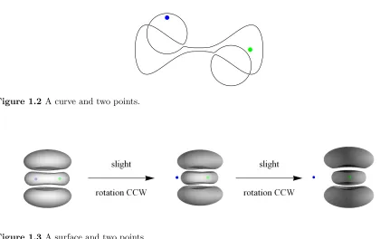
Figure 1.2 A curve and two points. . . 2

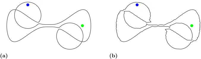
Figure 1.3 A surface and two points. . . 2

Figure 1.5 Plotting f = 0 using different numbers of sample points, where f is from (1.4). . . 4

Figure 1.10 Sample inputs for Problem 1.7. . . 7

Figure 1.11 Connectivity and Destination algorithms. . . 10

Figure 1.13 Illustration of Step 2 of Connectivity. . . 11

Figure 1.14 Illustration of the points inR. . . 12

Figure 1.15 Illustration of step 5 of Connectivity. . . 13

Figure 1.16 Illustration of steps 7 and 8 of Connectivity. . . 15

Figure 1.21 Illustration of various steepest ascent paths. . . 17

Figure 1.26 Illustration of the contours of a routing functiong along with its routing points. . . 19

Figure 1.29 Illustration of the outgoing eigenvectors of (Hessg)(r2). . . 19

Figure 1.32 Illustration of a connectivity path connectingp and q. . . 21

Figure 1.39 A sample connectivity path connectingp and q. . . 22

Figure 1.46 Illustration of the ridge and valley set ofg. . . 24

Figure 1.48 Illustration of several superlevel sets ofg. . . 26

Chapter 2 Partial Correctness . . . 27

Figure 2.3 Illustration of the stable manifolds for the routing points of g. . . 28

Figure 2.23 A decomposition of a connected component ofg. . . 36

Chapter 3 Termination . . . 39

Figure 3.12 Illustration of how to avoid the “bad” set of parameters. . . 45

Chapter 4 Length Bound . . . 47

Figure 4.1 Illustration of Ω curve. . . 48

Figure 4.33 Illustration of the induction base case. . . 61

Figure 4.34 A connected component containing more than one routing point. . . 62

Figure 4.35 Superlevel set of routing point lowest in height. . . 63

Figure 4.37 Illustration of pointsx0 _and _y0_{. . . 64}

Figure 4.38 Illustration of pointsx0 and y0. . . 65

Figure 4.39 Illustration of Case 1.1.1. . . 66

Figure 5.3 Illustration of the connectivity path for examples with n= 2. . . 71

Figure 5.5 Illustration of the connectivity path for example with n= 2. . . 75

(10)

Figure 5.10 Illustration of the connectivity path for example withn= 3. . . 78

Figure 5.14 Plot of the data from Table 5.13. . . 82

Chapter 6 Conclusion and Outlook . . . 84

(11)

Chapter 1

Introduction

Let us begin by looking at Figure 1.1.

Figure 1.1 A circle and two points.

Ask yourself the following question.

Q1: Can I draw a continuous curve starting at the blue point and ending at the green point without crossing the black curve?

We can immediately see that the answer is yes. Let us look at an example that is a little more complex. Ask yourself the same question after studying Figure 1.2. The answer in this instance is no. Answering the question might have been a bit more difficult because of the narrow gaps in the curves.

(12)

CHAPTER 1. INTRODUCTION

Figure 1.2 A curve and two points.

Figure 1.3 A surface and two points.

Q2: Can I draw a continuous curve starting at the blue point and ending at the green

point without crossing the gray surface?

The answer to the question is no. It may be difficult to tell from the pictures, but the green point lies inside one of the blobs while the blue point lies outside of all three blobs. Unfortunately, we cannot generalize this question to higher dimensions because we are unable to visualize higher dimensional surfaces very well.

Now rather than relying on pictures to describe our curves and surfaces, let us represent these objects using polynomials. We will represent a curve by a single polynomial equation in two variables and will represent a point by a tuple of numbers. We can rephrase question Q1 in the following way.

Q3: Can I draw a continuous curve starting at(p1, p2)and ending at (q1, q2) without

crossing f(x1, x2) = 0?

In Figure 1.1, the black circle represents the curve f(x1, x2) = 0 where f =x21+x22−1. The

(13)

by hand that

f(−1,1)>0 and f(1,1)>0,

and conclude that there exists a curve connecting the two given points without crossing f = 0. Hence the answer to question Q3 would be yes. Question Q3 becomes more difficult to answer when the polynomial f is more complicated. For example, the black curve in Figure 1.2 is the set of points where f(x1, x2) = 0 and

f = 4096x16₁ −16384x14₁ + 26624x12₁ −22528x10₁ −1024x8₁x4₂+ 1024x8₁x2₂ + 10496x8₁+ 2048x6₁x4₂−2048x6₁x2₂−2560x6₁−1280x4₁x4₂+ 1280x4₁x2₂ + 256x4₁+ 256x2₁x4₂−256x2₁x2₂−4096x16₂ + 16384x14₂ −26624x12₂ + 22528x10₂ −10560x8₂+ 2688x₂6−352x4₂+ 32x2₂−1.

(1.4)

Determining whether there exists such a curve connecting the two points −1 2,

1 2

(blue point) and 4₅,0 (green point) without crossing f = 0 is quite difficult now. It turns out that the answer is no in this instance. It is trivial to generalize question Q3 to higher dimensions:

Q4: Can I draw a continuous curve starting at (p1, p2, p3) and ending at(q1, q2, q3)

without crossing f(x1, x2, x3) = 0?

In Figure 1.3, we draw the surface f(x1, x2, x3) = 0 where

f =x6₁+ 4x4₁x2₂+ 3x₁4x2₃+ 2x4₁+ 5x2₁x4₂+ 8x2₁x2₂x2₃+ 8x2₁x2₂+ 3x2₁x4₃−12x2₁x2₃ −4x2₁+ 2x6₂+ 5x₂4x2₃+ 6x4₂+ 4x2₂x4₃−24x2₂x2₃+x₃6−14x4₃+ 28x2₃−7

and draw the points (0,2,0) (blue) and 4₅,0,0 (green). Again, determining whether we can connect the given points using a curve that avoidsf = 0 is a very difficult problem. As before, the answer is no.

(14)

answers. For instance, in Figure 1.5 we draw the curve f = 0 using the ContourPlotcommand in Mathematica, where f is from (1.4). In Figure 1.5a, many more sample points are used to draw the curve while far fewer sample points are used to draw the curve in Figure 1.5b. As mentioned earlier, we cannot connect the blue and green point in Figure 1.5a by a continuous curve that does not cross the black curve. However, it appears that in Figure 1.5b that we can connect the blue and green points by a continuous curve that does not cross the black curve. This discrepancy was caused by how we drew the curve f = 0.

(a) (b)

Figure 1.5 Plottingf = 0 using different numbers of sample points, wheref is from (1.4).

Questions like Q3 and Q4 are called connectivity queries. The white region in which the two points lie is called a semi-algebraic set. We are interested in determining whether two given points in a semi-algebraic set can be connected by some continuous curve. Notice that the black curve in Figure 1.5a splits the white region into four distinct regions. These four regions are called semi-algebraically connected components. An alternative formulation of questions Q3 and Q4 is to determine whether the two given points lie in a same semi-algebraically connected component.

(15)

1.1. PROBLEM STATEMENT CHAPTER 1. INTRODUCTION

geography [LaV06]. The field of motion planning was first introduced in scientific literature by Lozano-Perez, Wesley, and Reif [LPW79; Rei79].

In a broad sense, determining whether two points lie in a same connected component of a semi-algebraic set is part of a growing field called algorithmic real algebraic geometry [Bas03]. Real algebraic geometry is concerned with studying the properties of semi-algebraic sets. Computing properties such as the connected components of a semi-algebraic set is a fundamental problem and motivated the problem of computing the topology of semi-algebraic sets (see for example [SS83]).

In this thesis we present a robust symbolic-numeric method based on gradient ascent for deciding whether two given points in a semi-algebraic set are connected; that is, whether the two points lie in a same semi-algebraically connected component. In particular, we consider the semi-algebraic set defined byf 6= 0 where f is a given polynomial. In this chapter we will describe the symbolic part of the method and in a forthcoming paper, describe the numeric part of the method. The symbolic part of the method was first discussed in [Hon10]. The second part of the thesis focuses on proving the partial correctness and termination of the symbolic method assuming the correctness of the numeric subalgorithm. In the third part of the thesis we give an upper bound on the length of a path connecting the input points if they lie a same semi-algebraically connected component. In the last part of the thesis we give experimental timing results for our method.

In the first section we give a formal statement of the problem we will be studying in this thesis. In the second section we give an overview of the previous work done on this and related problems. In the third section we state the steps of the symbolic-numeric algorithm. Finally, in the fourth section we explicitly state the results in the thesis. They will be described in full detail in the chapters following.

1.1 Problem Statement

(16)

1.1. PROBLEM STATEMENT CHAPTER 1. INTRODUCTION

We say S is asemi-algebraic set in Rn if it is a finite union of sets of the form

  x∈R

n

P(x) = 0∧ ^

Q∈Q

Q(x)6= 0

  

where P is a polynomial inR[x1, . . . , xn] and Qis a finite subset ofR[x1, . . . , xn]. Let{f ?0} be

a shorthand notation for{x∈Rn|f(x)?0} where?∈ {=,6=, >, <,≥,≤}. A semi-algebraic set

S is semialgebrically connected ifS is not the disjoint union of two non-empty semi-algebraic sets that are both closed inS. A semi-algebraically connected component of a semi-algebraic set S is a maximal semi-algebraically connected subset of S. A semi-algebraic set has a finite number of semi-algebraically connected components. Throughout this thesis, when we use the shorthand notation ofconnected component, we mean a semi-algebraically connected component of a given semi-algebraic set.

Example 1.6. For f ∈R[x1, x2] defined by

f =−2x2

1+x41−2x22+ 2x21x22+x42

the set{f 6= 0} is a semi-algebraic set that has two (semi-algebraically) connected components.

We now state our problem precisely.

Problem 1.7.

Input: f ∈Z[x1, . . . , xn],n≥2, degf ≥1, squarefree, with finitely many singular points,

p, q∈_Qn_{∩ {f} ₆_{= 0}_}_.

Output: true, if and only if the two pointsp and q lie in a same connected component of the set {f 6= 0}.

Example 1.8. We illustrate the problem using a toy example. Let

f =−2x2

1+x41−2x22+ 2x21x22+x42. (1.9)

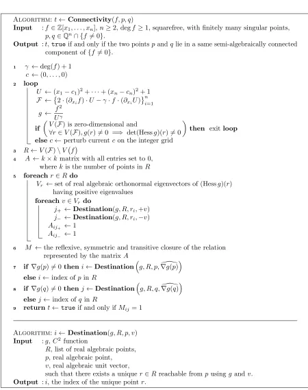
Figure 1.10a shows the set defined by f = 0. The two points p, q in Figure 1.10b cannot be connected via a continuous path in{f 6= 0}since they belong to different connected components. Hence the output should befalse. The two pointsp, qin Figure 1.10c, however, can be connected

(17)

1.2. PREVIOUS WORK CHAPTER 1. INTRODUCTION

(a)

p

q

(b)

p

q

(c)

Figure 1.10 Sample inputs for Problem 1.7.

1.2 Previous Work

Initially, it was not even clear as to whether the problem of rigorously determining whether two points lie in a same connected component of a semi-algebraic set S ⊂Rn was decidable. Evidence that the problem was decidable came in the form of the works by Tarski [Tar51] and Seidenberg [Sei54], who proved the decidability of the first order theory of real closed fields. Since then, there has been intense research effort on development of algorithms for performing quantifier elimination in the first order theory of real closed fields. A major breakthrough came in the form of the cylindrical algebraic decomposition algorithm developed by Collins [Col75], which used single variable resultants to perform quantifier elimination. Schwartz and Sharir [SS83] recognized the power of the cylindrical algebraic decomposition algorithm and used it to answer connectivity queries.

(18)

1.3. ALGORITHM CHAPTER 1. INTRODUCTION

In the previous papers, the construction of a roadmap of S ⊂ Rn depends on singly exponential many recursive calls to itself on several (n−1) dimensional slices of S. Improving the algorithms in those papers was a notoriously difficult problem with no progress made until very recently. In the papers by Basu, Roy, Safey El Din, and Schost [Bas12; BR13; SEDS10; SEDS13], they used an improved recursive scheme to drop the dimension by more than one in each recursive call.

All of the algorithms discussed so far are based on real algebraic geometry computations, which are difficult to implement and may not be fast in practice. This inspired researchers to search for practical solutions to solving motion planning problems using heuristic or sampling based approaches. In these approaches, completeness of the method is sacrified. One such method was based on potential fields [Kha86]. The idea was to create a scalar function, called the potential function, such that the gradient direction points away from the obstacle barrier. One can then follow the gradient field via gradient ascent (or descent) to traverse the free space. Typically the potential function is dependent on the input configurations; that is, the potential function is chosen in such a way that the goal configuration is a global minimum of the potential function.

A good middle ground between the symbolic approaches mentioned earlier and purely numeric approaches mentioned in the previous paragraph are hybrid symbolic-numeric methods. Recently, Iraji and Chitsaz [IC14] have proposed a method for computing a roadmap using a symbolic-numeric scheme. Their scheme bounds the roadmap using a chain of adjacent boxes, with each containing a slice of the roadmap. The method, called NuRA, preserves completeness of the roadmap algorithm and numerical experiments indicate it is practical.

In 2010, Hoon Hong [Hon10] published a note detailing a symbolic-numeric method for solving the problem (Problem 1.7) we are studying in this thesis. We present this method in the next section. The note did not provide a proof of partial correctness or termination. The method presented by Hong was unique in the sense that it answered connectivity queries using gradient trajectories, like in potential field methods, which typically are transcendental.

1.3 Algorithm

(19)

second subsection describes only the input/output specification of Destination.

1.3.1 Description of Algorithm Connectivity

We will illustrate the steps of Connectivity using the toy problem given in Example 1.8. We provide several pictures in the hope of aiding intuitive understanding of what each step does. Of course, the algorithms do not draw the pictures. We state the steps of Connectivity in Figure 1.11. We use the following notation. For a family F = {f1, . . . , fn} of polynomials in Z[x1, . . . , xn], we letV(F) denote the zero-locus inRnof the polynomials inF. For aC2 function

g we let Hessg denote the Hessian matrix of g. For a non-zero vectorv, we letvb= _kv_v_k where k·kis the Euclidean norm.

Example 1.12. Input. f =−2x2

1+x41−2x22+ 2x21x22+x42, p= (19/5,−1/2), q= (−9/10,−14/5) are the blue

and green points in Figure 1.10c, respectively.

• Here,n= 2, degf = 4, and f is a squarefree polynomial with exactly one singular point at (0,0).

1. Initially, we have

γ = 5, c= (0,0).

2. In the first iteration of the loop we have

U =x2₁+x2₂+ 1,

F =−2x5₁−4x2₂x3₁+ 20x₁3−2x4₂x1+ 20x22x1−8x1,

−2x5₂−4x2₁x3₂+ 20x3₂−2x4₁x2+ 20x21x2−8x2 ,

g= −2x

2

1+x41−2x22+ 2x21x22+x42

2

x2

1+x22+ 1

5 .

(20)

Algorithm:t←Connectivity(f, p, q)

Input :f ∈_Z[x1, . . . , xn],n≥2, degf ≥1, squarefree, with finitely many singular points,

p, q∈_Qn_{∩ {}_f ₆_{= 0}_}_.

Output :t,trueif and only if the two pointspandqlie in a same semi-algebraically connected component of{f 6= 0}.

1 γ ←deg(f) + 1

c ←(0, . . . ,0) 2 loop

U ←(x1−c1)2+· · ·+ (xn−cn)2+ 1 F ←2·(∂xif)·U−γ·f ·(∂xiU)

n i=1

g ← f 2

Uγ

if

V(F) is zero-dimensional and

∀r∈V(F), g(r)6= 0 =⇒ det(Hessg)(r)6= 0

then exit loop elsec←perturb currentc on the integer grid

3 R←V(F)\V f

4 A ←k×kmatrix with all entries set to 0, wherek is the number of points inR

5 foreachr∈R do

Vr ←set of real algebraic orthonormal eigenvectors of (Hessg)(r)

having positive eigenvalues foreachv∈Vrdo

j+ ←Destination(g, R, ri,+v)

j₋ ←Destination(g, R, ri,−v)

Aij+ ←1 Aij− ←1

6 M ←the reflexive, symmetric and transitive closure of the relation represented by the matrixA

7 if ∇g(p)6= 0theni←Destination

g, R, p,∇\g(p) elsei←index of pin R

8 if ∇g(q)6= 0thenj←Destination

g, R, q,∇\g(q) elsej←index of qinR

9 returnt←true if and only ifMij = 1

Algorithm:i←Destination(g, R, p, v) Input :g,C2_function

R, list of real algebraic points, p, real algebraic point,

v, real algebraic unit vector,

such that there exists a uniquer∈Rreachable from pusingg andv. Output :i, the index of the unique pointr.

(21)

(a) (b)

c1

c₂

(c)

Figure 1.13 Illustration of Step 2 of Connectivity.

second iteration of the loop we updateU,F andg to be

U =x2₁+ (x2−1)2+ 1,

F =−2x5₁−4x2₂x3₁−16x2x31+ 28x31−2x42x1

−16x3₂x1+ 28x22x1+ 16x2x1−16x1,

−2x5₂−6x4₂−4x2₁x₂3+ 28x3₂+ 4x₁2x2₂−4x2₂ −2x4

1x2+ 28x21x2−16x2+ 10x41−20x21 ,

g= −2x

2

1+x41−2x22+ 2x21x22+x42

2

x2

1+ (x2−1)2+ 1

5 .

The newV(F) is zero-dimensional. We illustrate the perturbedV(F) as the five red points in Figure 1.13b along with the contours for the newg. For all fiver∈V(F), four satisfy g(r)6= 0, and det(Hessg)(r)6= 0 at each of those four. Hence we exit the loop.

• One method for perturbing is using graded lexicographic order, which we visualize in Figure 1.13c. If there is an arrow having tip at α and tail atβ then xα_{> x}β _{in the} graded lexicographic order. We can follow the arrows to systematically change (c1, c2)

starting at (0,0). This generalizes, of course, to any number of variables.

• One can use standard symbolic computation methods to check whetherV(F) is zero-dimensional and to compute the real algebraic points in it. Furthermore, the elements of Hessg are rational functions with integer coefficients, so the determinant can be computed as well.

(22)

Figure 1.13b.

r

1

r

2

r

3

r

4

Figure 1.14 Illustration of the points inR.

• Note that each connected component of{f 6= 0}contains at least one point from the setR.

• One may observe from the contour plot ofg, that the pointsR are critical points of g whereg is non-zero.

• Again, we can use standard symbolic computation methods to identify which of the points inV(F) satisfy f = 0, and then remove them.

4. We have A=

     

0 0 0 0 0 0 0 0 0 0 0 0 0 0 0 0

    

 sincek= 4.

5. Supposer=r1 orr =r4. The matrix (Hessg)(r) has no positive eigenvalues. HenceVr =∅ and the body of the secondforeachloop does not execute.

Suppose instead that r = r2 or r = r3, then the matrix (Hessg)(r) has one positive

eigenvalue. For this eigenvalue, there are two corresponding real algebraic unit eigenvectors. Ifr =r2, the two eigenvectors are [−1 0]T and [1 0]T. We draw these two vectors as a dark

green and light green outward pointing arrow fromr2 in Figure 1.15a. Ifr=r3,

the two eigenvectors are [−1 0]T _{and [1 0]}T_{. We draw these two vectors as a dark blue}

and light blue outward pointing arrow fromr3 in Figure 1.15a. Rather than

(23)

we will use an arrow.

r

2

r

3

(a)

r

1

r

2

r

3

r

4

(b)

Figure 1.15 Illustration of step 5 of Connectivity.

We let

Vr2 =

n o

and Vr3 =

n o

.

Figure 1.15b shows four steepest ascent paths as red curves. Two of the red curves originate from r2. We see that steepest ascent from r2 in the initial direction approaches r4.

Similarly, we see that steepest ascent from r2 in the initial direction approaches r4.

Hence whenr =r2, the inner foreachloop executes once because there is only one vector

inVr2 and

j+←Destination

g, R, r2,

= 4, j−←Destination

g, R, r2,

= 4, A24←1,

A24←1.

Two of the other steepest ascent paths originate from r3. We see that steepest ascent from

r3 in the initial direction approaches r1. Similarly, we see that steepest ascent from

(24)

executes once because there is only one vector inVr3 and

j+←Destination

g, R, r3,

= 1, j−←Destination

g, R, r3,

= 1, A31←1,

A31←1.

The matrix A has the form

A=      

0 0 0 0 0 0 0 1 1 0 0 0 0 0 0 0

     .

• For eachr∈R, the Hessian (Hessg)(r) is a real symmetric matrix. It is a well known fact that the associated eigenvalues are all real and the eigenvectors corresponding to different eigenvalues are orthogonal. However, there is no restriction that the eigenvalues be simple, so it is possible that the geometric multiplicity of a positive eigenvalue is greater than one. In this case, finding two linearly independent eigenvectors for a given positive eigenvalue will suffice, as one can use the Gram-Schmidt process to find an orthonormal basis.

• Using standard symbolic computation techniques, we can find the eigenvalues and eigenvectors exactly because each point in R is an algebraic number and the elements of Hessg are rational functions with integer coefficients and the denominator is non-vanishing.

• Note that every steepest ascent path approaches a point in the set R. In fact, g was constructed to ensure that the path never spirals in a bounded region or goes forever into the infinity.

• It is crucial to observe that every two points inR can be connected if and only if they are connected via the above computed paths.

6. We have M =

     

1 0 1 0 0 1 0 1 1 0 1 0 0 1 0 1

     .

(25)

same connected component of{f 6= 0} by checking the (i, j) entry ofM. • We callM a connectivity matrix.

7. For the input pointp shown in Figure 1.16, ∇g(p)6= 0. We draw the vector_∇g\₍_p_{) as the}

p

q

r

1

r

2

r

3

r

4

Figure 1.16 Illustration of steps 7 and 8 of Connectivity.

blue arrow . We see that steepest ascent from pin the initial direction approaches r4. Hence

i←Destination

g, R, p, = 4.

8. For the input pointq shown in Figure 1.16,∇g(q)6= 0. We draw the vector _∇g\₍_q_{) as the} green arrow . We see that steepest ascent fromq in the initial direction approaches r4. Hence

j ←Destination

g, R, q, = 4.

9. We note thatM44= 1 and thus the two pointsp,q can be connected. We set t= true.

Output. t=true.

As an overview, the algorithm Connectivity consists of three main stages.

1. Usingf, compute “interesting” points on each connected component of{f 6= 0}. Create a function gwith desirable properties, one being that g= 0 if and only if f = 0. Use g and the “interesting” points to form some vectors.

(26)

3. Determine the connectivity of pand q usingN and trajectories of∇g by making use of Destinationonce again.

The first and second stage are much more time-consuming than the third one. Fortunately, one needs to carry out the first and second stage only once for a given f, since it depends only on f.

1.3.2 Specification of Subalgorithm Destination

In this subsection, we will describe the input/output specification of a certified numeric subal-gorithm called Destination, whose steps will be described a forthcoming paper. We begin by introducing some definitions.

Definition 1.17. Let g:Rn → R be a C2 function. Let p be a point in Rn and v be a unit vector inRn. We say φ is a trajectory of ∇g ifφ:I →Rn is aC2 function whereI is a finite union of open intervals of Rsuch that

φ0(t) =∇g φ(t)

and g◦φ:I →Ris injective. The pieces of the image φ(I) are calledsteepest ascent paths. We sayφis a trajectory of∇g through p using v ifφ: (0,∞)→_Rn_{is a} _C2 _{function and}

∀t >0 φ0(t) =∇g φ(t) and φ0(t)6= 0 (1.18)

and

lim

t→0+φ(t) =p

and

lim t→0+

φ0(t) kφ0₍_t₎_k =v

andg◦φ: (0,∞)→_Ris injective. We call the image φ (0,∞) asteepest ascent path through p usingv and denote this as SA(g, p, v). We call dest(φ) a destination of φif the following limit exists:

dest(φ) = lim t→∞φ(t).

We say a pointq ∈Rn is reachable from p using g and v if there existsφ, a trajectory of∇g through p usingv, such that dest(φ) =q.

Example 1.19. Let

g= −2x

2

1+x41−2x22+ 2x21x22+x42

2

x2

1+ (x2−1)2+ 1

(27)

1.4. OVERVIEW OF RESULTS CHAPTER 1. INTRODUCTION

and v = [−1 0]T_{. In Figure 1.21a we illustrate SA(}_{g, r}

2, v) as the red curve, where v is the

arrow. We see the point r4 is reachable fromr2 usingg and v. Letv=∇g\(p). In Figure 1.21b

we illustrate SA (g, p, v) as the blue curve, wherev is the arrow. We see the pointr4 is reachable

from pusing g and v.

r

2

r

4

(a)

p

r

4

(b)

Figure 1.21 Illustration of various steepest ascent paths.

We state the specification for the algorithm Destinationin Figure 1.11 and give a sample input and output in the following example.

Example 1.22. Letg be as in (1.20). Let andR,v be the set of points in red and the vector shown as the arrow in Figure 1.21a, respectively. Letp=r2. The pointr4 is the unique point

that is reachable fromr2 using gand v. Hence the output of Destination(g, R, p, v) would be

4.

1.4 Overview of Results

In this section we give an overview of the results in this thesis. We first give an outline and then give more precise results in the following subsections. The proofs of the results will be presented in the corresponding chapters.

(28)

third result in the thesis is a bound on the length of a path connecting two points in a connected component of{f 6= 0}. Besides being an interesting question on its own, it is a possible first step toward completing a complexity analysis of Connectivity. We present this bound in Chapter 4. We conclude the thesis with some computational results by executingConnectivity for various size inputs. These results will be presented in Chapter 5.

1.4.1 Partial Correctness

We will prove the partial correctness of Connectivity in Theorem 2.24. The proof essentially amounts to showing that any two “interesting” points in the same connected component of {g6= 0}are connected by a particular set of steepest ascent paths. In order to make the claim precise, we will need to recall and introduce some notations and notions.

Definition 1.23. Letg:Rn→Rbe a C2 function with n≥2. A critical pointp ofg is called a routing point of g if g(p) 6= 0. Let R be the set of routing points ofg. We call g a routing function if the following conditions are satisfied:

• For allx,g(x)≥0.

• For allε >0, there exists δ >0, such that for all x,kxk ≥δ impliesg(x)≤ε. • R is finite.

• For allx∈R,x is nondegenerate.

• The norms of the first and second derivatives ofg are bounded.

Intuitively, the second condition in the routing function definition says thatg vanishes at infinity; that is, askxk → ∞,g(x)→0.

Example 1.24. Let

g= −2x

2

1+x41−2x22+ 2x21x22+x42

2

x2

1+ (x2−1)2+ 1

5 . (1.25)

In Figure 1.26 we show the contours of g along with the routing points ofg as red dots. The black curve and black dot is the set of points where g= 0. One may easily check thatg satisfies the conditions to be called a routing function.

(29)

r

1

r

2

r

3

r

4

Figure 1.26 Illustration of the contours of a routing functiong along with its routing points.

Definition 1.27. LetA be a real symmetric matrix and letv be a unit eigenvector ofA with corresponding eigenvalueλ6= 0. We say v is an outgoing eigenvector ifλ >0.

Example 1.28. In Figure 1.29, the outgoing eigenvectors of (Hessg)(r2) are shown as arrows

pointing outward from the point r2. To be more precise,

(Hessg)(r2)≈

"

0.000198674 0 0 −0.000342484

#

and the vectors [1 0]T _{and [}₋_{1 0]}T _{are outgoing eigenvectors for (Hess}_g₎₍_r

2).

r

2

(30)

Definition 1.30. Let g:Rn → R be a C2 function with n ≥ 2. Let p, q ∈ Rn with p 6= q,

g(p)>0, and g(q)>0. We sayp and q are connected by steepest ascent paths using outgoing eigenvectors of g if there exist functionsφ1, . . . , φk+1 and routing pointsr1, . . . , rk such that

• if ∇g(p) = 0, then φ1 =pand r1 =p, otherwise, φ1 is a trajectory of ∇g throughp using \

∇g(p) and dest(φ1) =r1,

• if∇g(q) = 0, then φk+1=q andrk =q, otherwise,φk+1 is a trajectory of∇g throughq

using _∇g\₍_q_{) and dest(}_φ_k₊₁_{) =}_r_k_,

• for all 2≤i≤k, there exists an outgoing eigenvectorvi−1 of (Hessg)(ri−1) such thatφi is a trajectory of ∇g throughri−1 using vi−1 and dest(φi) =ri, or, there exists an outgoing

eigenvector vi of (Hessg)(ri) such that φi is a trajectory of∇g throughri usingvi and dest(φi) =ri−1.

Collectively, we call r1, . . . , rk and φ1, . . . , φk+1 a connectivity path for p and q.

Example 1.31. In Figure 1.32 we illustrate a connectivity for path p, qrepresented by r4,r2,

φ1,φ2,φ3. We describe whatφ1,φ2, andφ3 are now.

• Since∇g(p)6= 0,φ1 is a trajectory of∇gthrough pusing∇g\(p) where dest(φ1) =r4. The

blue curve is SAg, p,_∇g\₍_p₎_{and the light blue arrow is}_∇g\₍_p_).

• Since∇g(q)6= 0, φ3 is a trajectory of∇g throughq using∇g\(q) where dest(φ3) =r2. The

green curve is SAg, q,_∇g\₍_q₎_{and the light green arrow is} _∇g\₍_q_).

• The function φ2 is a trajectory of∇g throughr2 usingv (red arrow) which is an outgoing

eigenvector of (Hessg)(r2). We see dest(φ2) =r4. The red curve is SA(g, r2, v).

The partial correctness of the algorithm Connectivity relies heavily on the following theorem and is one of the main results in this thesis.

Theorem 1.33. If g is a routing function then any two points in a same connected component of {g6= 0} are connected by steepest ascent paths using outgoing eigenvectors ofg.

(31)

p

q

r

2

r

4

Figure 1.32 Illustration of a connectivity path connectingpandq.

1.4.2 Termination

The termination of Connectivity relies heavily on the following theorem, which is another one of the main results in this thesis.

Theorem 1.34. For all nonzero f ∈ _R[x1, . . . , xn] there exists a semi-algebraic set S ⊂ Rn

such that dim (Rn\S)< n and for all (c1, . . . , cn)∈S the mapping g:Rn→R defined by

g= f

2

(x1−c1)2+· · ·+ (xn−cn)2+ 1

deg(f)+1 (1.35)

is a routing function.

Intuitively, this theorem says there is a set of “bad” choices (Rn\S) for (c1, . . . , cn) which is

“small.” By choosing (c1, . . . , cn) outside of this “bad” set, the functiong in (1.35) is a routing

function. The proof of this theorem uses non-trivial results from semi-algebraic geometry such as Sard’s Theorem and the Constant Rank Theorem. We will use Theorem 1.34 to prove the termination of Connectivity in Theorem 3.13.

1.4.3 Length Bound

(32)

{f 6= 0}. To do so, we will bound the length of individual steepest ascent paths in a given ball. Before we can state the bound precisely, we introduce some notions.

Definition 1.36. Letg:Rn →Rbe aC2function withn≥2. Supposep, q∈Qnare connected by steepest ascent paths using outgoing eigenvectors ofg and denote byr1, . . . , rk, φ1, . . . , φk+1

a connectivity pathP forp and q. We define thelength of the connectivity path P to be k+1

X

i=1

Length(φi).

Example 1.37. Let

10x3

1−10x21+ 10x22−1

2

x2

1+x22+ 1

4 . (1.38)

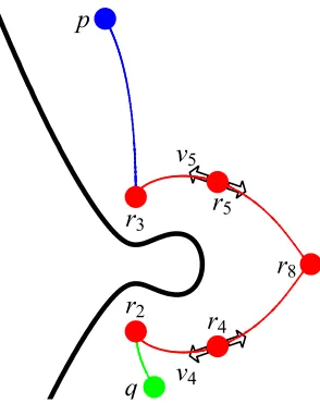
In Figure 1.39 we visualize a connectivity pathP given byr3, r5, r8, r4, r2,φ1, φ2, φ3, φ4, φ5, φ6for

pointspandqas the union of red steepest ascent paths and red routing points. The white arrows v4,−v4, v5,−v5 represent the outgoing eigenvectors of (Hessg)(r4), (Hessg)(r5), respectively,

that appear in the definition ofP. We give approximations of the lengths of six steepest ascent paths connectingp and q in Table 1.40. We approximate the length of the connectivty path P to be

2.97553 + 2·1.3696 + 2·1.96328 + 0.964633 = 10.6059.

r

2

r

3

r

4

r

5

r

8

p

q

v

5

(33)

Table 1.40 Approximate steepest ascent path lengths for a sample connectivity path connecting p andq.

φi Image ofφi Adjacent Points Approximate Length(φi) φ1 SA

g, p,_∇g\₍_p₎ _{p, r}₂ _2.97553

φ2 SA (g, r5, v5) r3, r5 1.3696

φ3 SA (g, r5,−v5) r5, r8 1.96328

φ4 SA (g, r4,−v4) r4, r8 1.96328

φ5 SA (g, r4, v4) r4, r2 1.3696

φ6 SA

g, q,_∇g\₍_q₎ _r₁_{, q} _0.964633

Definition 1.41. For a polynomial P ∈_Z[x1, . . . , xn] of the form

P =X E

aExE,

where E = (E1, . . . , En) runs over n-tuples of nonnegative integers and xE =xE11· · ·xEnn, we define theheight of P to be

hgt(P) = max E |aE|.

IfP ={P1, . . . , Pr} is a subset of Z[x1, . . . , xn], then we define theheight of P to be

hgt(P) = maxhgt(P1), . . . ,hgt(Pr) .

Example 1.42. Let

P1=x21+ 4x1x2−20x2+ 3,

P2= 2x21−4x1x2+ 3x1−1,

then

hgt(P1) = max

|1|,|4|,|−20|,|3| = 20, hgt(P2) = max

|2|,|−4|,|3|,|−1| = 4.

(34)

Definition 1.43. [Hof86] For a C2 _function _g_:

Rn→Rwe define the gradient extremal of g as Θ(g) ={x∈_Rn_{| ∃λ}_∈

R, (Hessg)(x)· ∇g(x) =λ∇g(x)}. (1.44)

Example 1.45. We illustrate Θ(g) for (1.38) as the blue curve in Figure 1.46a. In Figure 1.46b, we can observe that the set {g= 0} (black curve) and the routing points ofg (red points) are contained in Θ(g).

(a) (b)

Figure 1.46 Illustration of the ridge and valley set ofg.

An example of when Θ(g) is not a curve can be seen when

g= x

2 1+x22

2

x2

1+x22+ 1

3.

Here, Θ(g) =R2andgis not a routing function because the set of points(x1, x2)

x2

1+x22 = 2

are routing points ofg that are degenerate.

We now state the length bound result. A detailed proof will be given in Chapter 4.

Theorem 1.47. Let f ∈ _Z[x1, . . . , xn], n≥2, degree d≥2 with no singular points. Suppose (c1, . . . , cn)∈Zn such that

g= f

2

(x1−c1)2+· · ·+ (xn−cn)2+ 1

(35)

is a routing function. Let H = hgt(f). Let Θ(g) be the gradient extremal of g. Let D be a connected component of{f 6= 0} and p, q∈_Qn_∩_D_{. Let} _B _{be a ball of radius}

r=n 120A1A2Hd(c21+· · ·+c2n+ 1)

4n3₍₆_d₎3n

where

A1

A2

= min

   

g(p), g(q),

1

2dH c2

1+· · ·+c2n+ 2

104n3₍₅_d₎5n

    

is an irreducible fraction with A1, A2 >0. Suppose Θ(g)∩B is a compact rectifiable curve. Then

p and q can be connected in D by a connectivity path of length bounded by

4nr(6d+ 4)n−1.

The proof idea was motivated by the work of D’Acunto and Kurdyka [DK04]. The basic idea being that we can bound the length of a trajectory of∇gin a ball by bounding the length of Θ(g) in a ball. To find an appropriate sized ball, we use the simple observation that a connectivity path forp and q must be contained in{g≥ε} where

ε= ming(p), g(q), M

andM is the minimum value ofg(r) over all routing points r of g. For instance, for theg,p, and q given in Example 1.37, we visualize {g ≥g(p)},{g ≥g(q)}, and {g ≥M} as the blue, green, and red regions, respectively, in Figure 1.48. We see that

{g≥g(q)} ⊂ {g≥M} ⊂ {g≥g(p)}

and any connectivity path P forp and q must be contained in {g≥ε}={g≥g(p)}(the blue region).

1.4.4 Experimental Results

(36)

p

q

8 g

³

g

H

p

L<

8 g

³

g

H

q

L<

8 g

³

M

<

Figure 1.48 Illustration of several superlevel sets ofg.

(37)

Chapter 2

Partial Correctness

In this chapter, we will prove the partial correctness of the algorithmConnectivity in the form of Theorem 2.24. It essentially amounts to showing Theorem 1.33 is true. We assume throughout this section that g:Rn → R is a C2 function with n ≥ 2. The examples in this section will assume gtakes the form

g= −2x

2

1+x41−2x22+ 2x21x22+x42

2

x2

1+ (x2−1)2+ 1

5 .

In the first section we give some preliminary notions and lemmas necessary for proving Theo-rem 1.33. We then prove TheoTheo-rem 1.33 and the correctness of the algorithmConnectivity in the second section.

2.1 Preliminaries

To prove Theorem 1.33, we will use results motivated from the field of Morse theory. In Morse theory, one analyzes the topology of a manifold by studying differentiable functions on that manifold. In our case, we will be studying the manifoldRn and decomposing a region into sets of similar behavior based on trajectories.

Definition 2.1. Ifp∈Rn is a nondegenerate critical point of g, then the stable manifold of p is defined to be

Ws(p) ={x∈Rn|dest (φx) =p} ∪ {p}. where φx is the trajectory of ∇g through x using ∇g\(x).

(38)

2.1. PRELIMINARIES CHAPTER 2. PARTIAL CORRECTNESS

Example 2.2. Figure 2.3 illustrates the stable manifolds for the routing points ofg. The stable manifolds for r1 andr4 are the blue and green regions, respectively. The stable manifold for r2

is the blue line while the stable manifold forr3 is the green line.

--40242

-6

-4

-202

W

s

H

r4L

W

s

_H

_r1L

W

s

_H

_r2L

W

s

_H

_r3L

Figure 2.3 Illustration of the stable manifolds for the routing points ofg.

According to Figure 2.3, it appears we can decompose each connected component of {g6= 0} into a disjoint union of stable manifolds. We will use the following lemmas to show that if g is a routing function, we can in fact decompose a connected component into a disjoint union of stable manifolds. First, we observe the simple fact thatg strictly increases along a steepest ascent path.

Lemma 2.4. Let p∈_Rn_{. If} _p _{is not a critical point of} _g _then _g _{increases along a trajectory of} ∇g through p using _∇g\₍_p₎_.

Proof. Let p∈_Rn _with _∇g₍_p₎_{= 0. Let}₆ _φ_{denote a trajectory of} _∇g _through _p _using_∇g_\₍_p_{). We} have

d dtg φ(t)

=∇g φ(t), φ0(t)=∇g φ(t),∇g φ(t)=∇g φ(t)2. (2.5) Since pis not a critical point of g,∇g φ(t)2>0 for all t >0. It follows from (2.5) that

d dtg φ(t)

>0

for all t >0. Hence g strictly increases alongφ.

(39)

of {g6= 0}. First, we state some simple facts about g. Lemma 2.6. g is a bounded.

Proof. The first property in the definition of routing function guarantees g is bounded below by 0. Suppose for a contradiction that gis not bounded above. Then for all M, there existsx∈Rn such that |g(x)|> M. In particular, for everyn∈_N, there existsxn∈Rn for which|g(xn)|> n. Fix such a sequence {xn}∞n=1. Certainly,g(xn)≥0. Let

L= min n∈N

{g(xn)|g(xn)>0}, S={x∈_Rn|g(x)≥L}.

Let k be the index such that g(xk) = L. The second property in the definition of a routing function guaranteesS is bounded by lettingε=L >0. Since the tail{xn}∞n=k is contained inS, the Bolzano-Weierstrass theorem implies there exists a subsequence {xnj}

∞

j=1 which converges

to some limitM. Sinceg is continuous everywhere,

lim

j→∞g(xnj) =g(M). In particular, the sequenceg(xnj)

∞

j=1 is convergent, hence bounded. However, by construction,

g(xnj)

> nj ≥j for all j∈N, and hence this sequence is not bounded, a contradiction. Thus g is bounded above. Thereforeg is bounded.

Lemma 2.7. For all L >0,{x∈D|g(x)≥L} is compact.

Proof. Let L >0 and K={x∈D|g(x)≥L}. Recall thatg is bounded (Lemma 2.6), hence there existsM, such that for allx∈Rn,|g(x)| ≤M. The set

S=g−1 _[_{L, M}_]₌_{x_∈

Rn|g(x)≥L}

is closed because it is the preimage of a closed set under a continuous function and bounded due to the second property ofg being a routing function (lettingε=L >0). Therefore,Sis compact. The semi-algebraic set {g >0} is a disjoint union of open semi-algebraic connected components D1, . . . , Dk whereD1 =D (without loss of generality). SinceL >0,S is contained in{g >0}

and hence the disjoint union of D1, . . . , Dk. It follows that K =D∩S is compact.

(40)

Lemma 2.8. Let p∈D. If ∇g(p)6= 0, then there exists a unique trajectory φof ∇g through p using _∇g\₍_p₎

Proof. Let p ∈ D. The component D is an open subset of Rn containing p and g ∈ C2(D). According to the Fundamental Existence-Uniqueness Theorem [Per01, Section 2.2, pp. 74], there existsa >0 such that

φ0(t) =∇g φ(t)

φ(0) =p (2.9)

has a unique solution φ(t) on the interval [−a, a]. Let [0, β) be the right maximal interval of existence ofφ(t).

Because g is bounded (Lemma 2.6), the trajectory φ is bounded. It follows from [Per01, Theorem 3, Section 2.4, pp. 91] that β =∞. Certainly limt→0+φ(t) =pand

lim t→0+

φ0(t)

kφ0₍_t₎_k =∇g\(p).

Hence φis the trajectory of ∇g through p using_∇g\₍_p_).

Remark 2.10. A similar argument to the one above shows that ifp∈D and ∇g(p)6= 0 then there exists a unique C2 _function_φ_{: (}_−∞,_0]_→

Rn satisfying

φ0(t) =−∇g φ(t) φ(0) =p.

Combined with the argument above, this means that there exists a uniqueC2_function_φ_:

R→Rn satisfying (2.9). When ∇g(p) = 0, φ =p is the unique solution to (2.9), which exists for all t∈_R. We can conclude that the gradient vector field ∇g is complete.

Next, we have the important observation that the destination of every steepest ascent path is a routing point of g.

Lemma 2.11. Let p∈D with ∇g(p)6= 0 and φbe the trajectory of ∇g through p using _∇g\₍_p₎_.

Then dest(φ) exists and is a routing point of g in D.

Proof. Letp∈Dwith∇g(p)= 0 and6 φbe the trajectory of ∇g throughp using _∇g\₍_p_{), whose} existence is guaranteed by Lemma 2.8. LetK ={x∈D|g(x)≥g(p)}. Lemma 2.7 impliesK is compact. Let{tn} ⊂R+ be a sequence with limn→∞tn=∞. Let

_e

(41)

so that φ etn ⊆K for all n. The sequence

φ etn is an infinite set of points in a compact set, so it has an accumulation point q.

First, we show q is a critical point of g. It suffices to show ∇g φ(t) → 0 as t → ∞. Differentiating φ0(t) we find

φ00(t) =∇∂

∂φ∇g φ(t)

φ0(t) =∇∂

∂φ∇g φ(t)

∇g φ(t)

(2.12)

holds for all t >0. The first and second derivatives of g are bounded because g is a routing function, hence we may deduce from (2.12) that φ0 _{is uniformly Lipschitz continuous for} _{t >}_0.

Since g is bounded (Lemma 2.6),g∞:= limt→∞g φ(t)

<∞, and for 0< t <∞

g∞≥g φ(t)> g(p),

so from (2.5) _Z ∞

0

kφ0(t)k2dt=

Z ∞

0

d dtg φ(t)

dt=g∞−g(p)<∞. (2.13) Since φ0 is uniformly Lipschitz continuous, (2.13) implies

lim

t→∞∇g φ(t)

= lim t→∞φ

0 (t) = 0

as desired.

We claim dest(φ) = limt→∞φ(t) = q. Since nondegenerate critical points are isolated [BH04, Lemma 3.2, Section 3.1, pp. 47], we can pick a closed neighborhood U of q where q is the only critical point of U. Suppose for a contradiction limt→∞φ(t) 6= q, then there is an open neighborhood V ⊂ U of q and a sequence {sn} ⊂ R+ with limn→∞sn = ∞ and φ(sn)∈U \V ⊆U\V. Thus, the sequence {φ(sn)} has an accumulation point in the compact set U\V which, as above, must be a critical point ofg. This contradicts the choice of U, and therefore, dest(φ) =q.

Finally, we show q is a routing point in D. We find g(q) > g(p) >0 because g increases along φast→ ∞ (Lemma 2.4). Hence,q ∈D is a routing point.

We now show that the connected components of {g6= 0} can be decomposed in to a disjoint union of stable manifolds.

(42)

routing points contained in D; that is,

D= a

p∈RD

Ws₍_p₎_.

where RD is the set of routing points of g in D.

Proof. LetRD be the set of routing points ofginD. Letq∈Dbe arbitrary. Certainlyq ∈Ws(q), so we may assume ∇g(q)6= 0. Letφdenote the trajectory of ∇g throughq using_∇g\₍_q_{), whose} existence is guaranteed by Lemma 2.8. It follows from Lemma 2.11 that there exists a routing point r ∈ RD such that dest(φ) = r. Hence q ∈ Ws(r). This shows D is a union of stable manifolds. It is a disjoint union due to the uniqueness ofφ.

Now that we have a decomposition, the next natural question to ask is whether we can determine the dimension of each stable manifold. The definition of a stable manifold relies on a critical point, so one may believe that the dimension relies on the index of the critical point. To see this, we use the Stable Manifold Theorem, a fundamental result in the field of dynamical systems.

Lemma 2.15. If p ∈ D is a routing point of g with index k, then Ws₍_p₎ _{is a smooth} _k

-dimensional manifold.

Proof. Let pbe a routing point of indexk of gcontained in D. The result in [BH04, Theorem 4.2, Section 4.1, pp. 94] has the same conclusion but the assumptions are that g is a Morse function defined on a finite dimensional compact smooth Riemannian manifold. The function g restricted toDis Morse becausegis a routing function. The connected componentDof{g6= 0} is a finite dimensional smooth Riemannian manifold, but it is not compact. The compactness assumption is used in several spots throughout the proof of the cited theorem.

(1) There exist finitely many critical points ofg on the given manifold [BH04, Corollary 3.3, Section 3.1, pp. 47].

(2) The gradient vector field∇g generates a unique 1-parameter group of diffeomorphisms defined onR×D [BH04, Section 4.1, pp. 94].

(3) The destination of a trajectory is a critical point [BH04, Corollary 3.19, Section 3.2, pp. 59].

(43)

(1) The manifold Dcontains finitely many routing points because g is a routing function. (2) This follows from the fact that the gradient vector field∇g is complete (Remark 2.10). (3) This is exactly Lemma 2.11.

We expect all the routing points in a connected component to be connected via steepest ascent paths, so we expect each component to have a “peak” to ascend to; that is, we expect each component to have a local maximum. The simple observation follows from the routing function properties.

Lemma 2.16. The component D contains a routing point of g having indexn.

Proof. Take x0 ∈D. Then g(x0)>0. LetK ={x∈D|g(x)≥g(x0)}. The set K is compact

(Lemma 2.7), hence g has a maximumz onK. The maximum must occur on the interior of K. If the interior is non-empty, then there exists an open ball B aroundz such that g(z)≥g(x) for all x∈B. Hence z is a local maximum ofg; that is, z is a routing point having indexn. If the interior is empty, choosex1∈Dsuch that g(x1)< g(x0), which is possible due to the second

property of g being a routing function. Let Ke ={x∈D|g(x)≥g(x1)}. Again, the set Ke is

compact sog has a maximumz_eon K. The interior ofKe is non-empty, so as argued before,z_eis a local maximum ofg; that is _ezis a routing point having index n.

Throughout this section we will use the notation ∂W to denote the boundary of a stable manifold W.

Lemma 2.17. If p is a routing point of g of index n, then ∂Ws₍_p₎ _{contains no routing points}

of indexn.

Proof. Letpbe a routing point ofgof indexn. Assume for a contradiction that∂Ws₍_p_{) contains} a routing pointq of indexn. Hence q is a local maximum ofg. Any neighborhoodU ofq must contain a point y∈Ws₍_p_{) where} _g₍_y₎_{> g}₍_q_{), contradicting the fact that}_q _{is a local maximum.} Hence,∂Ws₍_p_{) contains no routing points of index}_n_.

Lemma 2.18. Let r ∈ D be a routing point of g of index n. Let p ∈ ∂Ws₍_r₎_∩ _D _with ∇g(p) 6= 0 and φ be the trajectory of ∇g through p using _∇g\₍_p₎_{. Then there exists a routing}

pointq ∈∂Ws₍_r₎_∩_D _{such that} _dest(_φ_{) =}_q_.

(44)

p ∈Ws₍_q_{). In fact, all the points along SA}_{g, p,}_∇g_\₍_p₎_{are in} _Ws₍_q_{). Since} _φ _{is continuous} and D is a disjoint union of stable manifolds (Lemma 2.14), we find thatq ∈∂Ws₍_r_{). Thus} q∈∂Ws₍_r₎_∩_D_{as desired.}

Lemma 2.19. Letr ∈D be a routing point of g of indexn. Letp∈∂Ws₍_r₎_∩_D_{be a routing}

point of g of index strictly less than n. If v is a outgoing eigenvector of (Hessg)(p) tangent to ∂Ws₍_r₎_{, then there exists a routing point}_q _∈_∂Ws₍_r₎_∩_D _{that is reachable from} _p _using _v_.

Proof. Letr ∈D be a routing point ofg of index n. Let p∈∂Ws₍_r₎_∩_D _{be a routing point of} g of index strictly less thann. Letv be a outgoing eigenvector of (Hessg)(p) tangent to∂Ws₍_r_). As argued in the proof of Lemma 2.15, we may use the conclusions of the Stable Manifold Theorem [BH04, Theorem 4.2, Section 4.1, pp. 94]. This theorem guarantees the existence of the unstable manifold

Wu(p) ={x∈_Rn|dest (φx) =p} ∪ {p}.

whereφxis the trajectory of−∇gthroughxusing−∇g\(x). There exists a submanifold ofWu(p) that is tangent to the eigenspace spanned by outgoing eigenvectors of Hessg(p). In particular, this submanifold corresponds to SA(g, p, v). For each sin SA(g, p, v), ∇g(s)6= 0. We can argue using Lemma 2.11 that there exists a routing pointq ∈Dsuch that for each sin SA(g, p, v), dest(φs) =qwhereφsis the trajectory of∇gthroughsusing∇g\(s). In particular,qis reachable fromp usinggandv. Certainlyq ∈D. Since SA(g, p, v) is a continuous curve andDis a disjoint union of stable manifolds (Lemma 2.14), we find that q ∈∂Ws₍_r_{). Thus} _q _∈ _∂Ws₍_r₎_∩_D _as desired.

Lemma 2.20. Let r ∈D be a routing point ofg of index n. Let q be a routing point of g on ∂Ws₍_r₎_∩_D_{. Then} _q _{is connected to} _r _{by steepest ascent paths using outgoing eigenvectors of}_g_.

Proof. Letr ∈Dbe a routing point ofgof index n. Letqbe a routing point ofgon∂Ws₍_r₎_∩_D_. According to Lemma 2.17, q must be a routing point of index strictly less than n. Hence, (Hessg)(q) has at least one outgoing eigenvector, call itv.

If v is not tangent to ∂Ws₍_r_{), then SA(}_{g, q, v}_{) or SA(}_{g, q,}_−v_{) lies in the stable manifold} Ws₍_r_{) because} _D _{is a disjoint union of stable manifolds (Lemma 2.14). Hence}_r _{is reachable} from q using v (or −v). We see q is connected to r by steepest ascent paths using outgoing eigenvectors ofg.

If v is tangent to ∂Ws₍_r_{), according to Lemma 2.19 there exists another routing point} _q

2

that is reachable from q=q1 using v. The routing point q2 has index strictly less thann, so as

(45)

2.2. PROOF OF MAIN RESULT CHAPTER 2. PARTIAL CORRECTNESS

The functiong is bounded (Lemma 2.6) and there are finitely many routing points, so eventually the process will terminate, and we will find a routing point qk,k≥1, where (Hessg)(qk) has an outgoing eigenvectorvk that is not tangent to∂Ws(r). The pointr is reachable fromqk usingg and vk as before. We have found a sequence of routing points q1. . . , qk,k≥2 such that qi is reachable from qi−1 usingg and an outgoing eigenvector of (Hessg)(qi−1). Thus the point q is

connected tor by steepest ascent paths using outgoing eigenvectors ofgby the connectivity path q1, . . . , qk, rand the corresponding trajectories connecting the routing points q1, . . . , qk, r. Definition 2.21. Let p, q ∈ D, p 6= q, be routing points of g of index n. We say Ws₍_p_{) is}

adjacent toWs₍_q_{) if} _D_∩_∂Ws₍_p₎_∩_∂Ws₍_q_{) is non-empty.}

Lemma 2.22. Let p, q∈D, p6=q, be routing points of g of index n. If Ws₍_p₎ _{is adjacent to} Ws₍_q₎_{, then} _D_∩_∂Ws₍_p₎_∩_∂Ws₍_q₎ _{must contain a routing point of}_g_.

Proof. Let p, q∈D,p6=q, be routing points ofgof indexn. AssumeZ =D∩∂Ws₍_p₎_∩_∂Ws₍_q₎ is non-empty. Suppose Z does not contain a routing point ofg. As Z is non-empty, there exists a point x∈Z that is not a routing point of g. According to Lemma 2.18, there exists a routing point q∈Z. However, this contradicts our assumption. Hence, Z contains a routing point of g.

2.2 Proof of Main Result

In this section we will prove Theorem 1.33 and prove the partial correctness of Connectivity in the form of Theorem 2.24.

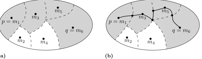
Proof of Theorem 1.33. Let R denote the set of routing points of g in D andp, q ∈D, p6=q be arbitrary. We will show p and q are connected by steepest ascent paths using outgoing eigenvectors of g. We may assume without loss of generality thatp and q are routing points of g, otherwise we can always ascend to one using Lemma 2.11 if ∇g(p) 6= 0 or ∇g(q) 6= 0. Let m1, . . . , m` denote the routing points inR having index n. We see `≥1 due to Lemma 2.16. We see that|R|>1 becausep andq are both distinct routing points ofg.

Suppose first that `= 1. According to Lemma 2.15, Ws₍_m

1) isn-dimensional and the stable

manifolds for the points in R\ {m1} have dimension strictly less than n. As D is a disjoint

union of stable manifolds of the routing points in R (Lemma 2.14), it follows that the points in R\ {m1}lie on ∂Ws(m1). We see for all r∈R\ {m1}, r is connected to m1 by steepest ascent

(46)

Now suppose ` >1. According to Lemma 2.15, for all i,Ws₍_m

i) isn-dimensional and the stable manifolds for the points inR\ {m1, . . . , m`}have dimension strictly less than n. Ifp (or q) is a routing point with index strictly less thann, then it must lie on the boundary of some stable manifoldWs₍_m_{i). According to Lemma 2.20, we can connect} _p _(or_q_{) to} _m

i by steepest ascent paths using outgoing eigenvectors. Hence, we may assume without loss of generality that p andq are routing points having indexn. We will connect p andq by looking at a sequence of adjacent stable manifolds of dimensionnas seen in Figure 2.23a.

p=m1

m2

m3

m4

m5

q=m6

(a)

p=m1

m2

m3

m4

m5

q=m6

(b)

Figure 2.23 A decomposition of a connected component ofg.

It suffices to show that we can connect any two mi, mj whose stable manifoldsWs(mi) and Ws₍_m

j) are adjacent becauseD is a disjoint union of stable manifolds of the routing points in R (Lemma 2.14). From Lemma 2.22, we know two adjacent manifolds have a routing point in common in their boundary. According to Lemma 2.20, we can connect this common routing point to both mi and mj by steepest ascent paths using outgoing eigenvectors. Hence we can connectmi andmj by steepest ascent paths using outgoing eigenvectors. We illustrate this in Figure 2.23b. This completes the proof of Theorem 1.33.

Theorem 2.24. Algorithm Connectivity is correct.

Proof. Let f, p,q be the inputs to Connectivity satisfying the specification. Suppose Con-nectivity terminated with outputt. Let

g= f

2

Uγ whereU = (x1−c1)

2₊_{· · ·}_{+ (}_x

n−cn)2+ 1, γ= deg(f) + 1

(47)

routing points ofg. We observe that

∇g= f

Uγ+1(2∇f U −γf∇U) (2.25)

so

R={x∈_Rn| ∇g(x) = 0, g(x)6= 0}

={x∈_Rn|2∇f(x)U(x)−γf(x)∇U(x) = 0, f(x)6= 0}.

Let F = 2∇f U −γf∇U. We see that the V(F) contains exactly the routing points ofg and the singular points of f becauseU is non-zero. In step 3, we remove the finitely many singular points of f from V(F), leaving us with the correct set of routing points. The set of routing points is finite becauseV(F) is zero-dimensional.

We now claim that g is a routing function. The function g is C2 _{because it is a rational}

function where the denominator is nonnegative. According to step 2, the finitely many routing points of g are all nondegenerate because det(Hessg)(r) 6= 0 for all r ∈ R. The choice of γ = deg(f) + 1 guarantees the property thatg vanishes at infinity (property two) because the degree of the numerator is smaller than the degree of the denominator. Certainly the function g is nonnegative. To understand why the first derivative ofg is bounded, we observe in (2.25) that each component of ∇gis a rational function where the degree of the numerator is smaller than the degree of the denominator, which is nonnegative. A similar argument holds for each component of Hessg. Henceg satisfies the properties in the definition of a routing function.

Observe thatg= 0 if and only iff = 0. Due to Theorem 1.33, we know the routing points of g on a connected component of {f 6= 0}are connected by steepest ascent paths using outgoing eigenvectors of g. It is important to observe that these steepest ascent paths do not cross f = 0 due to Lemma 2.4. In steps 5 and 6, we use the certified Destinationalgorithm to determine which routing points are adjacent to one another via steepest ascent paths using outgoing eigenvectors. The matrixA is the adjacency matrix for the graph whose vertices are the routing points and whose edges are the steepest ascent paths connecting them. Hence, the matrixM, the reflexive, symmetric, transitive closure ofA, satisfies the condition that Mij = 1 if and only ifri, rj ∈R lie in a same connected component of{f 6= 0}.

(48)

(49)

Chapter 3

Termination

In this chapter, we will prove that the termination of the algorithmConnectivity in the form of Theorem 3.13. For this, we must show that the perturbation step completes after a finite number of iterations. We will show in Theorem 1.34 that there is only a small (measure zero) set of parameters for which the functiongformed inConnectivityis not a routing function. Hence we are guaranteed to find a routing function by finitely many perturbation of these parameters on the integer grid.

In the first section we state some preliminary notions and a lemma used in the proof of The-orem 1.34. In the second section we prove TheThe-orem 1.34 and show the algorithmConnectivity terminates.

3.1 Preliminaries

We begin by recalling defintions from semi-algebraic geometry [Bas03]. LetA⊂_Rm _and_B_⊂ Rn be two semi-algebraic sets. A functionf:A→B issemi-algebraic if its graph is a semi-algebraic subset ofRm+n. For openA, the set of semi-algebraic functions fromAtoB for which all partial derivatives up to order `exist and are continuous is denoted S`₍_{A, B}_{). The class}_S∞₍_{A, B}_{) is} the intersection ofS`₍_{A, B}_{) for all finite} _`_{. A}_S∞_{-diffeomorphism} _φ_{from a semi-algebraic open} U ⊂_Rn _{to a semi-algebraic open} _V _⊂

Rn is a bijection fromU toV such that φ∈ S∞(U, V) and φ−1 _{∈ S}∞₍_{V, U}_).

Let `≥0. A semi-algebraicA⊂_Rn_{is a} _S∞_{-submanifold of}

Rn of dimension `if for every