Analyzing Longitudinal Data with Non-ignorable Missing

(1)

ZHU, LIANSHENG. Analyzing Longitudinal Data with Non-Ignorable Missing. (Under the direction of Dr. Sujit Ghosh and Dr. Subhashis Ghosal.)

(2)

efficiency. When the missingness does depend on the patterns, results based on simulated data suggest that both approaches yield accurate estimates if the underlying number of patterns is specified correctly. Otherwise the PI method leads to biased results whereas the JM approach still provides reasonably accurate estimates.

(3)

(4)

by

LIANSHENG ZHU

A dissertation submitted to the Graduate Faculty of

North Carolina State University

In partial fulﬁllment of the

Requirements for the degree of

Doctor of Philosophy

STATISTICS

Raleigh, NC

2006

APPROVED BY

Sujit Ghosh, Co-Chair Subhashis Ghosal, Co-Chair

(5)

(6)

Biography

Liansheng Zhu was born in Qidong, a coastal town in the Eastern China. He graduated

from Huilong High School at Qidong in 1994. He received a Bachelor of Sciences degree

in Chemistry and Chemical Engineering from Hunan University at Changsha, China in

1998. He obtained a Master’s of Sciences degree in Statistics from Kansas State University

at Manhattan, Kansas in 2003. He then joined the graduate program in the Department

of Statistics at North Carolina State University in August 2003. He is working as a

(7)

Acknowledgements

First, I would like to express my deepest appreciation to my wonderful advisors Dr. Sujit

Ghosh and Dr. Subhashis Ghosal for their guidance, training and support during this

research. It is my honor to have them as my advisors, to learn and get inspiration from

them. Also, I am grateful to the valuable suggestions and comments from Dr. Anastasios

Tsiatis and Dr. Hao Zhang on this research and their presence in my committee. Many

thanks also go to Dr. Jie Zhang in Novartis Pharmaceuticals from whom I got inspiration

to initiate this research. Finally, I want to thank my dearest parents, sister and brother,

for their endless love and support. Special thanks also go to my parents-in-law who come

(8)

List of Tables

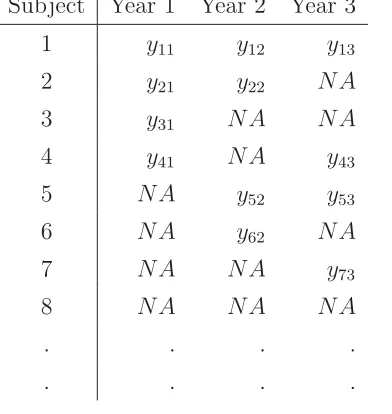
1.1 The typical data structure. (N A: missing data) . . . 3

2.1 Proportion of data simulated in the ﬁrst scenario . . . 19

2.2 Comparison of Bias’s and SE’s of estimates for the scenario 1. FA: the

full-data analysis. PI3, PI6, and PI12: the pseudo-imputation methods

with 3, 6, and 12 patterns, respectively. . . 21

2.3 Comparison of two versions ofDIC’s. DIC1 (Spiegellhalter et al., 2002)

and DIC2 (Gelman et al., 2003). . . 22 2.4 Comparison of estimates and their SE’s for ﬁxed eﬀects in the R-model

from joint-modeling approach based on the scenario 1 . . . 23

2.5 Results of simulation for the joint modeling with the misspeciﬁcation of

the distribution for random patterns. . . 26

4.1 Parameter estimates and their standard errors from analyzing aids data

by utilizing various methods. * indicates the fixed effect is significant at

the signiﬁcance level α= 0.05 . . . 45 4.2 Parameter estimates and their standard errors from analyzing aids data

(11)

List of Figures

2.1 Parameter estimates from 4 methods under Scenario 1. FA, the full-data

analysis. LOCF, the last observation carried forward method. PI3, the

pseudo-imputation method with 3 patterns. JM3, the joint-modeling

ap-proach with 3 patterns. . . 20

2.2 Parameter estimates of ﬁxed eﬀects in the Y-model from joint-modeling

approach with diﬀerent patterns under Scenario 1. . . 22

2.3 Partial parameter estimates under Scenario 2. . . 25

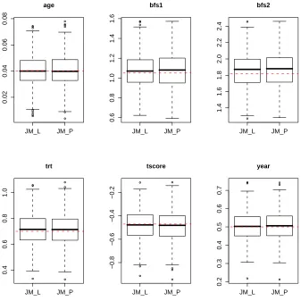
2.4 Comparison of results betweenJ M_L and J M_P with 3 patterns under Sce-nario 1. J M_L, the joint model with the use of the logistic regression in the

R-model; J M_P, the use of the probit regression in the R-model . . . 28

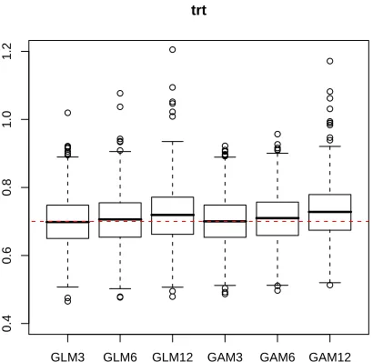
3.1 Parameter estimates for covariates “trt” (top) and “tscore” (bottom) in

the ﬁrst simulation. GLM: the generalized linear model and GAM: the

generalized additive model at the ﬁrst step of the PI method. 3, 6 and 12

indicated the number of patterns speciﬁed for both methods. The dashed

horizonal line indicates the true value of β. . . 36 3.2 Parameter estimates for covariates “age” (top) and “year” (bottom) in

(12)

3.3 Parameter estimates for covariates “bfs1” (top) and “bfs2” (bottom) in

horizonal line indicates the true value of β. . . 38

3.4 Smooth estimate of age . . . 39

3.5 Parameter estimates of treatment eﬀects from the PI approach with

diﬀer-ent modeling techniques. GLM: the generalized linear model and GAM:

the generalized additive model at the ﬁrst step of the PI method. 3 and

6 indicated the number of patterns speciﬁed for both methods. The data

generation model is a GAM under Scenario 1. The dashed horizonal line

indicates the true value of β. . . 40 3.6 Parameter estimate of the treatment eﬀect from the JM approach with

GAM when data generated by a GAM under Scenario 1. The dashed

(13)

Chapter 1

Introduction

In longitudinal studies, measurements of a response variable and some explanatory

variables for each subject are recorded repeatedly across time. The primary interest

is often the estimation of either the change in the response variables over time or the

eﬀects of independent variables at the completion of studies. Longitudinal studies are

popular in epidemiological research. Besides that, they are gaining increasing popularity

in clinical trials of intervention dealing with chronic diseases. Although most studies are

well designed and every attempt is made to collect data on each subject at each of the

follow-up times, it is often unavoidable to have some measurements missing intermittently

and/or even have subjects dropped out prior to the completion of the study. The reasons

behind such missing may be study-related, for example, adverse event, competing risks,

lack of eﬀectiveness of treatments, or even early recovery. It can also be non-study

related, e.g., accidental death or moving away. An example of a longitudinal study is

given in Section 1.1. Section 1.2 provides notations and deﬁnitions for model description.

Some statistical methods in literature dealing with non-ignorable missing are discussed

in Section 1.3.

1.1

A Motivating Study

According to the National Osteoporosis Foundation, vertebral fractures are the most

(14)

fracture, one out of ﬁve will suﬀer their next vertebral fracture within just one year,

potentially leading to a fracture “cascade”. There is a three-year clinical trial in which

binary outcomes (new fracture versus no new fracture) of vertebral fracture are measured

at the end of each year. Baseline measurements include patients’ age, Tscore (calculated

from bone mineral density), and baseline fracture status (0, 1, ≥ 2). Patients are

ran-domly assigned to either the treatment group or the placebo group. Some patients may

not have any post-baseline measurements and some patients may only have incomplete

post-baseline measurements. In this speciﬁc study, it was deﬁned that if a fracture is

determined for the patient at the jth year, it will be assumed that his or her post jth

year outcome is a fracture as well since the vertebral fracture can not be cured (once

a fracture, always a fracture). Therefore, data from these patients are not counted as

missing even when there are no measurements available. That means the subjects are

considered as dropouts only if they do not experience fracture before missing. The

pri-mary analysis is to compare the intervention with the control on vertebral fracture based

on the population excluding patients without any post-baseline data. There is reason

to suspect that dropouts may depend on responses because subjects with new fractures

may be more likely to quit than those with no fractures. Hence, standard statistical

methods do allow the missing mechanism to depend on missing observations may yield

biased estimates and hence misleading conclusions might be drawn by the clinicians.

1.2

Notations and Definitions

Let Y_ij be the responses of theith subject measured at the jth time point, X_i denote

the vector of baseline covariates, andR_ij be the missing indicator variable fori= 1, . . . , n,

andj = 1, . . . , m. LetR_ij = 1 ifY_ij observed andR_ij = 0 otherwise. LetY be the matrix

of Y_ij’s andX andR be matrices of X_i’s, andR_ij’s. The variable Y can be expressed as

(Y_obs, Y_miss), where Y_obs denotes observed responses and Y_miss the missing ones.

Consider again the above example of the 3-year study. If subjects have at least one

post-baseline measurement, and then they are included in the analysis. Hence, there are

only three missing patterns since a monotonic missing mechanism (dropout) is observed.

(15)

Table 1.1: The typical data structure. (N A: missing data)

Subject Year 1 Year 2 Year 3

1 y₁₁ y₁₂ y₁₃

2 y₂₁ y₂₂ N A

3 y₃₁ N A N A

4 y₄₁ N A y₄₃

5 N A y₅₂ y₅₃

6 N A y₆₂ N A

7 N A N A y₇₃

8 N A N A N A

. . . .

can be eight possible missing patterns. A typical data structure is illustrated in Table 1,

where NA indicates a missing observation. In this illustration,R₁₁= 1, R₂₃= 0 etc.

In Rubin and Little’s taxonomy (1976, 1987), there are in general three missing

mechanisms that can be expressed in terms of the conditional distribution of R given X

and Y. Let f(U|V) denote the conditional distribution of U given V.

1. Missing completely at random (MCAR): f(R|X, Y) = f(R). One extension of

MCAR is deﬁned as the covariate-dependent MCAR iff(R|X, Y) = f(R|X).

2. Missing at random (MAR): f(R|X, Y) = f(R|Y_obs, X).

3. Non-ignorable missing (NIM): f(R|X, Y) =f(R|X, Y_obs, Y_miss).

The third mechanism (NIM) which makes no restrictive assumption on missing

mecha-nisms is the main focus of our research.

1.3

Models and Associated Methods for NIM Data

It is generally diﬃcult to model NIM data since the distributional assumptions about

(16)

otherwise. There is a large volume of literature devoted to reduce bias resulting from this

type of missing. Two widely used approaches are selection models and mixture models.

In mixture models, the joint density of repeated outcomes Y and missing indicator R,

conditional on covariates, X is written as f(Y, R|X) = f(Y|R, X)f(R|X) whereas for

selection models it is written as f(Y, R|X) =f(Y|X)f(R|Y, X).

1.3.1

Selection Models

Selection models, which were ﬁrst introduced in the univariate setting by Heckman

(1976) appearing in the econometrics literature, require one to combine a model for the

full data with a selection model for missing indicators given data. Diggle and Kenward

(1994) extended Heckman’s work to multivariate normal data. Fizmaurice et al. (1996)

proposed multivariate logistic models for incomplete binary responses while Molenberghs

et al. (1997) introduced methods for analyzing longitudinal ordinal data with

non-ignorable missing. In practice, one can assume a generalized linear regression model

for the full-data using a suitable linear function to explain eﬀects of covariates and a

logit or probit model for the selection model.

Selection models are intuitively appealing since the inference about parameter

es-timates of primary interest can be obtained directly from f(Y|X), and parameters in

f(R|Y, X) can be treated as nuisance parameters provided there are no common

para-meters in f(Y|X) and f(R|Y, X). However, some limitations do exist. For instance, for

continuous responses, the common assumption of multivariate normality is not easy to

verify when some responses are missing (Hogan et al., 2004). Moreover, the selection

model postulated to model the dependence of dropout process on unobserved responses

is not veriﬁable. Inference from selection models can be highly sensitive to model

as-sumptions (Little and Rubin, 2002). Finally, computations can be very intensive due to

general requirement of likelihood maximization and numerical instability occurs resulting

from the possibility of a ﬂat likelihood about the parameters of primary interest (Hogan,

(17)

1.3.2

Pattern-mixture Models

Although the terminology of pattern-mixture models that are our main focus here

was ﬁrst deﬁned by Little (1993), the early application of mixture concepts can be traced

back to Rubin (1977). Conventionally, marginalization of results are often in need. For

example, Little (1993, 1994) and Molenberghs et al. (1998) ﬁrst stratiﬁed the incomplete

data by missing patterns, then ﬁtted distinct models within each stratum, and ﬁnally

summarized results over patterns. The general model can be written as

f(Y, R|X) =f(Y|R, X)f(R|X), (1.1)

where the distribution ofY, conditional onR andX, is multinomial and R is treated as

a covariate, and the distribution of R given X can be left unspeciﬁed or in a parametric

form. Marginalization over patterns is required to obtain estimates of parameters of

primary interest.

Traditionally, missing patterns are deﬁned according to times to missing. For

ex-ample, there are eight patterns for a typical data set like the one shown in Table 1.1.

Without a doubt, it is often unavoidable that not all parameters are estimable because of

some missing observations. In other words, pattern-mixture models are under-identiﬁed

(Little 1993). Either restriction must be set for some patterns, additional assumptions

be made, or information need to be borrowed from observed data. To overcome the

under-identiﬁable problem, Wu and Bailey (1988, 1989) allow responses to depend on

missing indicators through individual random eﬀects estimated from a general linear

mixed model, then average over the distribution of random eﬀects that can be assumed

to be parametric or left unspeciﬁed. The model can be written as

f(Y, R|X) =

f(Y|b, X)f(R|b, X)dF(b), (1.2)

where b is the subject-speciﬁc random parameter vector. The variables Y and R are

linked throughband inference can be made based on (Y|b, X) by integrating outb. This

model is often called shared parameter (SP) model. Follmann and Wu (1995) extended

(18)

responses without any parametric assumption on random eﬀects. Estimation of marginal

means for binary cases was described by Birmingham and Fitzmaurice (2002).

Guo et al. (2004) proposed a random pattern-mixture model for continuous data

in which they considered dropout patterns as random latent variables and determined

according to many factors, including times to missing, baseline covariates and/or

time-varying covariates. The key assumption of this model is that the longitudinal responses,

Y, are independent of the missing indicators, R, conditional on the pattern eﬀects. The

proposed model is given by,

f(Y, R, b|X) =

f(Y|b, X, u, R)f(b|X, R, u)f(R|u, X)f(u|X)du

=

f(Y|b, X, u)f(b|X, u)f(R|u, X)f(u|X)du, (1.3)

wherebis the subject-speciﬁc random parameter vector anduis the latent variable vector

representing the random pattern eﬀect. To obtain parameters of primary interest, one

requires marginalization over b and u which can be computationally diﬃcult. To avoid

this task, a joint normal approach was adopted and maximum likelihood estimates were

derived by EM algorithm.

As will be seen, marginalization is often required. It may not be that problematic

if responses are continuous and/or the ﬁnal parameter of interest is the marginal mean.

However, in situations where there are a number of covariates of interest in discrete

longitudinal data, methods for parameter-wise marginalized results can be very tricky.

For instance, suppose that there are two covariates, treatments and patients’ age, denoted

as X₁ and X₂, respectively. Also, suppose that there are two missing patterns. Then, a

logistic regression is usually ﬁt for binary data conditional on each missing pattern,

P(k)= (1 + exp[−(β₀(k)+X₁(k)β₁(k)+X₂(k)β₂(k))])−1. (1.4)

where k is the pattern indicator, 1 or 2. Obviously, β₁(k) is the logarithm of odds ratio

between two treatments given the value of age and the pattern k. However, what we

need is a marginal parameter β₁ to measure the eﬀect of treatment irrespective of the

(19)

as β₁(k)’s. The above methods that are available in the literature do not provide such

marginal parameter β₁ such that the marginalized estimates of parameters are still of

meaningful representation as the conditional estimates based on patterns.

To resolve both the under-identiﬁability and marginalization problems, we propose

two approaches in the Chapter 2. The ﬁrst one will be called the pseudo imputation (PI)

approach, an approximation method for estimating parameters at the marginal level.

Secondly, we extend the method proposed by Guoet al.(2004) to general cases by jointly

modeling Y and R within a Bayesian framework and will be called the joint-modeling

(JM) approach. Both methods are applicable to both discrete and continuous outcomes.

At this moment, it is assumed that a surrogate variable is observed and missing patterns

are known. Simulation studies are conducted to illustrate the proposed methods and

to compare them with some exiting methods. In Chapter 3, we extend our approaches

to accommodate more general situations and relax the assumptions in Chapter 2. In

Chapter 4, the proposed methods are illustrated using a real life data set from an aids

(20)

Chapter 2

Proposed Statistical Methods

Firstly it is assumed that a surrogate variable determining missing patterns is fully

observed. Then, we deﬁne Z_i, that has a known distribution, as the design matrix of

missing patterns with the random eﬀect u_i. We further assume f(R_ij|Y_ij, X_i, Z_i, u_i) =

f(R_ij|X_i, Z_i, u_i), which means that the missing mechanism is conditionally MAR given

the latent variableu_i. For a given pattern, data often contain both observed responses and

missed ones, the problem of under-identiﬁability, which is encountered by the traditional

pattern-mixture models that use time to dropout as patterns, does not exist any more.

The models presented in this chapter are general enough in the sense of that we do not

require the assumption of monotonic or intermittent missingness pattern. The

pseudo-imputation (PI) method and its extension will be described in Section 2.1, followed by

the joint modeling (JM) method. In Section 2.3, simulation studies based on diﬀerent

scenarios are carried out. Section 2.4 presents conclusions and some general remarks.

2.1

The Pseudo-imputation (PI) Method

2.1.1

Model Description

The ﬁrst step is to estimate E(Y_ij|X_i, Z_i) = µ_ij and its corresponding variance within

each pattern for both observed and missing subjects. Standard methods can be used for

(21)

As it is well-known in the multiple imputation technique, more than one values are

sim-ulated for each missing point based on estimated E(Y_ij|Z_i, X_i) and its variance that are

obtained at the ﬁrst step. On the contrary, the pseudo-imputation method does not

im-pute the missing values but directly models estimatedE(Y_ij|Z_i, X_i) or its transformation

in linear regression framework. By doing so, estimates of marginal parameters can be

obtained. In summary, the following three steps are needed to implement the PI method:

1. Given Z_i, estimate µ_ij by using a standard method (e.g., GLMM).

2. Transform the estimate, sayh(ˆµ_ij), by using a desired functional form. For example,

logit for binary data and log for count data. By doing so,h(ˆµ_ij) will be linear inβ.

3. Fit a linear model

E(h(ˆµ_ij)|X_i) = X_iTβ (2.1)

where the estimate of β is indeed at the marginal level.

Notice that the variance of estimates obtained at Stage 3 is under estimated since it

ignores the fact that a major proportion of variation has been reduced at Stage 1. Hence,

we need to derive the variance of estimates for ﬁxed eﬀects, denoted as var( ˆβ). In linear

models, var( ˆβ) = (XTV−1X)−1, where,

V =var(h(ˆµ_ij)) =var(E(h(ˆµ_ij)|Z_i)) +E(var(h(ˆµ_ij)|Z_i)) (2.2)

If a linear mixed model is used at Stage 3 and u treated as random with mean 0 and

variance Ω, then E(var(h(ˆµ_ij)|u)) = ZTΩZ+ Σ where Ω and the random error Σ can be

estimated at the third stage and E(var(h(ˆµ_ij)|u)) at the ﬁrst stage. Therefore, var( ˆβ)

can be obtained without much diﬃculty. Explicit steps to get parameter estimates and

their corresponding variance are demonstrated in the following example.

2.1.2

Example

For illustration we consider the binary data described in Section 1. The original data

(22)

variable. Now, we can rewrite (Y_ij, X_i) as

Y_ij(k) ={Y_ij :S_i =k}

X_i(k) ={X_i :S_i =k} (2.3)

Suppose the variable, baseline fracture status (BFS), is a good surrogate for responses

and missing indicators and hence it links Y and R. Then, we can have three patterns

corresponding toS_i=BFS_i =k,k= 1,2,3. Hence, the ﬁrst step is to regressY_ij(k)onX_i(k)

and obtain βˆ(k) and ˆµ(_ijk). In this step, a logistic regression can be used since responses

are binary,

Y_ijk ∼Ber(P_ij(k))

µ(_ijk) =P_ij(k) = [1 + exp(−X_i(k)β(k))]−1. (2.4)

For instance,X_i(k) = (1,Tscore_i(k),year_i(k),trt(_ik),age(_ik))T. Notice that BFS is not included

in the model since there is only one level of BFS in each pattern by deﬁnition.

After obtaining the estimates of µ(_ijk), ˆµ(_ijk) at the ﬁrst step, the second step is to

transform ˆµ(_ijk) by the logit function, denoted ash(ˆµ(_ijk)), which is linear in β. Obviously,

h(ˆµ(_ijk)) = X_i(k)β(k). At the third step, the marginal estimate, ˆβ, will be obtained by using

a linear model for ˆµ(_ijk) and all covariates,

E(h(ˆµ(_ijk))) =X_iTβ, (2.5)

where X_iT = (1,Tscore_i,year_i,trt_i,age_i,BFS_i)T. The variance ofh(ˆµ(_ijk)) is given by

ˆ

V = ˆVar(h(ˆµ(_ijk))) = ˆVar(E(h(ˆµ(_ijk))|S_i)) + ˆE(Var(h(ˆµ_ij(k))|S_i)). (2.6)

Since the logit function is used at the second step, h(ˆµ(_ijk)) = X_i(k)βˆ(k). Hence,

ˆ

var(E(h(ˆµ(_ijk))|S_i)) = ˆΣ +STΩˆS

ˆ

(23)

WhereS is the vector of S_i’s. The estimate of variance-covariance matrix for the

within-pattern variation and the between-within-pattern variance ( ˆΣ and ˆΩ can be obtained at the

third step while Var( ˆβ(k)) is available at the ﬁrst step. LetV∗ be the matrix of Var( ˆβ(k)).

Therefore,var( ˆβ) = (XTVˆ−1X)−1 = (XT( ˆΣ +STΩˆS+V∗)−1X)−1.

2.1.3

Extension and Asymptotic Property

Previously, we assume there exists a desirable link function at the second stage of

the proposed method. However, it is not necessary. In the following, we are going to

construct the estimation equation and derive asymptotic properties in a general sense.

Denote the estimates of the predictive means obtained at the ﬁrst stage to be ˆµ_k and n_k

be the number of observations for the kth pattern. Notice that µ_k = µ under the true

model. Then the likelihood score equation for approximating β is

K

k=1

n_k

∂µ_k(β)

∂β

V_k−1(ˆµ_k−µ_k(β)) (2.8)

and the variance of the maximum likelihood estimator for ˆβ can be estimated by

K

k=1

n_k

∂µ_k(β)

∂β

V_k−1

∂µ_k(β)

∂β

_T ₋₁

(2.9)

Lemma 1. Suppose that β₀ is the true parameter and that

(i) n12

k(ˆµk−µk(β0)) has asymptotic distribution N(0, Vk) for k = 1, . . . , K,

ii) ∂µ_∂βk(β) and V_k for all k are continuous in the neighborhood ofβ₀ and the inverse of the

limit of

1

n

_K

k=1nk(∂µ_∂βk(β))Vk−1(∂µ∂βk(β))T

exists. Then,

(a) βˆ is consistent for β₀,

(b) n12( ˆβ−β₀) has an asymptotic normal distribution.

(24)

is equal to 0 and some regularity conditions are satisﬁed. The regularity conditions for

consistency can be found in Serﬂing (Chapter 4, 1980), Huber (Lemma 2.1 and Theorem

2.2 in Chapter 6, 1981) , and van der Vaart (Theorems 5.7 and 5.9, 1998). Here, we only

check if the expectation condition holds. Clearly, as the expectation is with respect to

β₀, E[(ˆµ_k−µ_k(β))|Z_k] = 0 as the condition (i) in Lemma 1 holds. Hence, with respect

toβ₀,

EK_k₌₁n_k(∂µk(β)

∂β )Vk−1(ˆµk−µk(β))|Zk = 0.

By conditional expectation, it results in

E{K_k₌₁n_k(∂µk(β)

∂β )Vk−1(ˆµk−µk(β))}= 0.

Therefore, ˆβ is the consistent estimator of β₀. To derive the large sample distributional

properties of the above estimator, one can follow the usual approach for the M-estimators

(25)

2.2

Joint Modeling

2.2.1

Model Description

We propose to use the following model,

µ_ij =E(Y_ij|X_i, Z_i, u_i, β) = g₁(X_iTβ+Z_iu₁_i) (2.10)

π_ij =E(R_ij = 1|u_i, X_i, Z_i, α) =g₂(X_iTα+Z_iu₂_i) (2.11)

u_i ∼F(.) (2.12)

where g₁ and g₂ are monotone link functions, the random eﬀects u_i = (u₁_i, u₂_i) have a

bivariate distribution which can be left unspeciﬁed. X_i is a known design matrix. The

parameter vectors β and α are unknown and β is of primary interest. u₁_i and u₂_i are

correlated random eﬀects with the design matrix Z_i for dropout patterns. Here we call

Model (2.10) as the Y-model and Model (2.11) the R-model. With the key assumption

off(Y|R, X, Z, u₁) = f(Y|X, Z, u₁), the joint distribution ofY and Rwithufor random

pattern eﬀects can be written as

(2.13)

Lemma 2. The proposed model (2.10) - (2.12) captures the dependence ofR on Y.

Proof. Notice that, under MAR, f(R|Y, X) = f(R|Y_obs, X) ⇔ f(Y_miss|Y_obs, R, X) =

(26)

Notice that,

f(Y|R, X) =

f(Y, u|R, X)du

=

f(Y|u, R, X)f(u|X, R)du

=

f(Y|u, X)f(u|X, R)du

=

f(Y|u, X)f(R|u, X)f(u|X)

f(R|X) du

=

f(Y|u, X)f(R|u, X)f(u|X)du

f(R, u|X)du (2.14)

and

f(Y_obs|R, X) = f(Yobs, Ymiss|u, X )f(R|u, X)f(u|X)dudYmiss

f(R, u|X)du (2.15)

Hence,

f(Y|R, X)

f(Y_obs|R, X) =

f(Y_obs, Y_miss|u, X)f(R|u, X)f(u|X)du

f(Y_obs, Y_miss|u, X)f(R|u, X)f(u|X)dudY_miss (2.16)

which can not be free of R in general. Therefore, our proposed model does capture the

dependency of R onY which is the key assumption of NIM.

For the purpose of illustration, we investigate the dependence of R on Y through

a numerical example by using Monte Carlo approximation. Suppose the univariate

re-sponses,Y_i ∼Ber(1, p_i) andR_i ∼Ber(1, π_i), where logit(p_i) = X_iTβ,βT = (β₀, . . . , β₅) =

(−6.9,−0.5,0.7,0.04,1,1.8) are true values,X_iT = (1,Tscore_i,trt_i,age_i,BFS_i)T, logit(π_i) =

−1.5−0.5x_i + 0.5Y_i and i = 1. . .100. Values of covariates are generated by the same way as in Section 2.3. By the data construction, R does depend on Y. Now, we would

like to see if our formulation captures the dependency. Equivalently, if _ff₍_Y(Y|R=1,X) obs|R=1,X) =

f(Y|R=0,X)

f(Yobs|R=0,X), then the ratio is free ofR. Otherwise, it is not. Given values of parameters, Equation (2.14) can be approximated by

f(Y|R, X)

f(Y_obs|R, X) ≈

N−1N_l₌₁f(Y_obs, Y_miss|u_l, X)f(R|u_l, X)

(27)

whereu_l has the bivariate standard normal distributions with correlation coeﬃcientρ=

0.6. For each given set of values of u_l, terms inside of summand can be evaluated. By

repeating itN = 5000 times, ratios that can be obtained with respect toRare 0.0099 and

0.0027. Clearly, they are diﬀerent. Hence, our proposed method captures dependency of

R on Y.

Let D_obs = (Y_obs, X, Z, R) denote the observed data. Write D = (Y, X, Z, R) and

thus D is not fully observed. For simplicity, let us assume u has the bivariate normal

distribution with mean 0 and variance-covariance matrix Σ_u. We consider independent

priors for β, α, and Σ_u, so that π(β, α,Σ_u) = π(β)π(α)π(Σ_u). Then, the joint posterior

of θ = (β, α,Σ_u) is

π(β, α,Σ_u|D_obs) =

f(Y_obs,ij|X_i, Z_ij, u_i)f(R_ij|X_i, Z_ij, u_i)f(u_i|X_i)

π(β, α,Σ_u).

(2.18)

In the above equation, β is the parameter of primary interest and α,Σ_u are considered

as nuisance parameters.

2.2.2

Prior Selection and Posterior Computation

The choice of prior distributions reﬂects information about unknown parameters. It

is desirable to pick mathematically manageable functions as prior distributions which

results in computationally convenient posterior distributions. Hence, conjugate prior

distributions are often desired. If responses are discrete as in our case, ﬁnding conjugate

priors can be hardly possible, particularly for parametersβandαin the proposed model.

Moreover, the data provide little information about the additional variance

compo-nents (Σ_u) for the latent variable - missing patterns. Therefore, the speciﬁcation of a

proper prior for Σ_u might be a crucial element in this missing-data problem. This prior

distribution should carry some degree of information, capturing a reasonable amount of

variation between dropout patterns and association betweenf(Y|X, Z, u) andf(R|X, Z, u).

Intuitively, a Wishart distribution with the scale matrix Q and the degrees of freedom

η can be a good candidate as the prior for the inverse of Σ_u. For priors of β and α, we

(28)

chosen resulting in nearly a non-informative prior.

To sample from the joint posterior distribution π(β, α,Σ_u|D_obs), a standard Gibbs

sampling algorithm obtains samples from the following conditional distributions: 1)

[β|α,Σ_u, D_obs], 2) [α|β,Σ_u, D_obs], and 3) [Σ_u|β, α, D_obs]. Closed forms of the above three

full conditional posterior distributions are not available. However, if these full

condi-tional distributions are log concave functions, we can use the adaptive rejection sampling

(Gilks, 1992). By construction, the above condition holds. Therefore, direct sampling

or derivative-free adaptive rejection sampling algorithm (Gilks, 1992) can be adopted to

draw samples from each of the above three conditional posterior distributions.

Convergence of MCMC samples is often an issue for Bayesian computing. Fortunately,

it can be easily checked in WinBUGS by looking at trace plots with running multiple

chains. In our cases two chains mix quite well after a few thousand samples from each

chain. Initial samples can be discarded as burn-in samples and then remaining iterations

can be retained to obtain approximate posterior estimates of the desired parameters.

Density plots can be obtained to summarize posterior distributions. Literature on how

to deal with these issues in MCMC samples includes Brooks (1998), Cowles and Carlin

(1996), and Gilks et al. (1996).

2.2.3

Model Selection

The joint-modeling approach requires determination of the number of patterns.

Ini-tially, we assume the underlying number of patters are known. In reality, it remains

unknown and ultimately needs to be determined. It can be determined arbitrarily or in a

purely data-driven way. Hence, it is critical to assess model adequacy that is the matter

of model selection. Here, we consider a Bayesian model selection criterion, namely, a

deviance information criterion (DIC) proposed by Spiegellhalter et al. (2002). It can be

used with informative, uninformative, and improper priors.

DIC is deﬁned as,DIC = ¯D(θ)+p_D, whereθis the vector of all parameters involved in

the model,p_Dis the estimated eﬀective number of parameters in the posterior distribution

given by p_D = ¯D(θ)−D(¯θ), and ¯D(θ) is the posterior mean of the deviance and D(¯θ)

(29)

−2 logf(y|θ) wheref(y|θ) is the likelihood. DIC can be easily obtained in WinBUGS. It had been observed that this deﬁnition proposed by Spiegellhalter et al. (2002) can

hardly be utilized due to that the R2WinBUGS program is not able to call the deviance

function because of WinBUGS called from the outside of R2WinBUGS (Sturtz et al.,

2005). Actually, it is available in R2WinBUGS program now. Instead, Sturtz et al.

(2005) adopted the deﬁnition of p_D introduced by Gelman et al. (2003, Section 6.7)

which is deﬁned as the half of the posterior variance of the Bayesian deviance. In other

words, DIC = ¯D(θ) + 1₂Var(ˆ D(θ)). An additional advantage of choosing this deﬁnition

is that p_D >0 even when ¯D(θ)< D(¯θ).

Gelman et al. (2003) noted that both deﬁnitions ofp_D can be derived from the

asymp-totic χ2 distribution of the deviance relative to its minimum. A model with the smallest

DIC will be chosen. Since both DIC’s can be easily obtained by using WinBUGS, we

will compare their performance in later simulation studies.

2.3

Simulation Study

To study the performance of proposed methods, we conduct a series of simulation

studies covering diﬀerent missing mechanisms. Data are simulated mimicking the study

described in Section 1.1. The full data are generated from the following model:

Y_ij ∼Ber(p_ij)

p_ij =1 + exp{−X_iTβ}−1 (2.19)

where βT = (β₀, . . . , β₆) = (−7.5,−0.47,0.5,0.7,0.04,1.05,1.82) are true values of

para-meters for covariates X_iT = (1,Tscore_i,year_i,trt_i,age_i,BFS_i)T, i = 1, . . . ,600 index for

subjects,j = 1,2,3 the time points. The values of Tscore and age for each individual are

generated fromN(−2.7,0.52) andN(73,5.42), respectively. The values of year_i = 1,2,or

3, trt_i = 1 or 0, and BFS_i = 1,2,or 3 are generated with equal probabilities. Then, a

sur-rogate variable, sayW_ij ∼N(S_iTβ∗,1), whereβ∗T = (−5.25,−0.4,0.35,0.02,0.63,1.27,0),

and S_iT = (intercept_i,Tscore_i,trt_i,age_i,bfs1_iI(BFS_i = 1),bfs2_iI(BFS_i = 2),year_i)T.

(30)

example, subjects with the values of W_ij’s within the ﬁrst 1/3 of the ordered W_ij’s are

allocated into the ﬁrst group, or Z_ij = 1.

After data are simulated, we ﬁt 9 models to each dataset. These model include the

full data analysis (FA), last observation carried forward (LOCF), pseudo-imputation (PI)

methods with 3 patterns (PI3), PI with 6 patterns (PI6), PI and with 12 patterns (PI12),

the joint modeling approach with 3 patterns (JM3), JM with 6 patterns (JM6), and JM

with 12 patterns (JM12), the shared-parameter model using the subject-speciﬁc random

eﬀect as the link between Y-model and R-model. For the joint modeling approach,

u is modeled as to have the bivariate normal distribution with a mean vector of 0’s

and a variance-covariance Σ_u. The prior distribution for both β and α is assumed to

be N(0,10−4) and for the inverse of Σ_u we use the Wishart distribution with the

2-dimensional identity matrix as the scale matrix and the degree of freedom of 2. For

each scenario considered, 500 data sets are generated. Models for generating missing

indicators are described in the following sections.

2.3.1

Results based on Scenario 1

In the ﬁrst scenario, the missing indicatorR_ij are generated using the following model:

R_ij ∼Ber(π_ij)

logit(π_ij) =α₀+α₁ ∗trt_i+α₂∗year_i+Z_iju_i (2.20)

where trt_i, a subvector ofX_i, denotes the treatment assignment, (α₀, α₁, α₂) = (−3.3,−0.5,0.1),

and u_i ∼ N(0,1.752). On average, 16% of data were found to be missing.

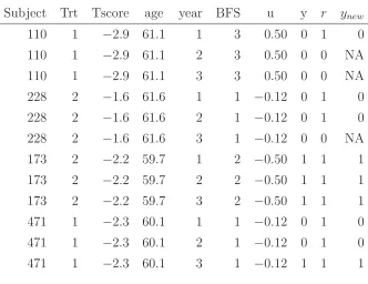
A portion of one simulated data set based on the ﬁrst scenario is given in Table 2.1.

As shown, some subjects fail to comply after the ﬁrst year, some after the second year,

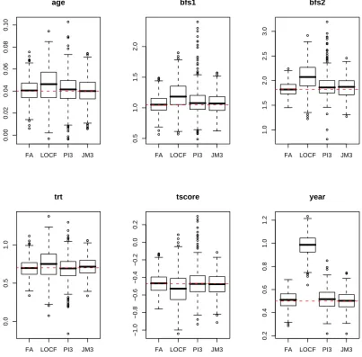
and some complete the study. Figure 2.1 summarizes the results for the ﬁxed eﬀects in

the Y-model from the FA, LOCF, PI3 and JM3 approaches. The dash lines indicate

true values of parameters. The LOCF method produces substantially biased estimates

for almost every ﬁxed eﬀect. On the other hand, the pseudo-imputation method and the

(31)

Table 2.1: Proportion of data simulated in the ﬁrst scenario

Subject Trt Tscore age year BFS u y r y_new

110 1 −2.9 61.1 1 3 0.50 0 1 0

110 1 −2.9 61.1 2 3 0.50 0 0 NA

110 1 −2.9 61.1 3 3 0.50 0 0 NA

228 2 −1.6 61.6 1 1 −0.12 0 1 0

228 2 −1.6 61.6 2 1 −0.12 0 1 0

228 2 −1.6 61.6 3 1 −0.12 0 0 NA

173 2 −2.2 59.7 1 2 −0.50 1 1 1

173 2 −2.2 59.7 2 2 −0.50 1 1 1

173 2 −2.2 59.7 3 2 −0.50 1 1 1

471 1 −2.3 60.1 1 1 −0.12 0 1 0

471 1 −2.3 60.1 2 1 −0.12 0 1 0

471 1 −2.3 60.1 3 1 −0.12 1 1 1

full-data analysis, when the number of patterns is correctly speciﬁed. Also, estimates

obtained from the pseudo-imputation method generally have larger variations than those

from the joint-modeling approach.

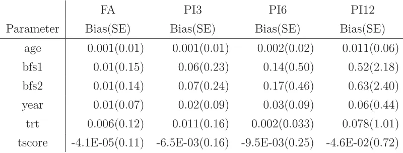
Table 2.2 shows biases and SE’s of estimates from the PI method with diﬀerent

number of missing patterns. The biases and SE’s appear to be larger as the number

of patterns increases except that the estimate of the treatment eﬀect has the least bias

when the number of patterns assumed to be 6. It implies that the PI method might

be very sensitive to the number of patterns chosen. When the number of patterns is

speciﬁed incorrectly, results can be very misleading, even if a right surrogate variable is

used and the missingness indeed depends on the random pattern variable controlled by

that surrogate variable.

Comparison of the joint-modeling approach with a diﬀerent number of patterns and

the SP model is given in Figure 2.2. The estimates appear to be approximately unbiased

despite the fact that JM model is based on the wrong number of patterns. The SP

model provides acceptable results, compared with the JM model. The estimates based

(32)

FA LOCF PI3 JM3 0.00 0.02 0.04 0.06 0.08 0.10 age

FA LOCF PI3 JM3

0.5

1.0

1.5

2.0

bfs1

FA LOCF PI3 JM3

1.0 1.5 2.0 2.5 3.0 bfs2

FA LOCF PI3 JM3

0.0

0.5

1.0

trt

FA LOCF PI3 JM3

−1.0 −0.8 −0.6 −0.4 −0.2 0.0 0.2 tscore

FA LOCF PI3 JM3

0.2 0.4 0.6 0.8 1.0 1.2 year

Figure 2.1: Parameter estimates from 4 methods under Scenario 1. FA, the

full-data analysis. LOCF, the last observation carried forward method. PI3, the

(33)

Table 2.2: Comparison of Bias’s and SE’s of estimates for the scenario 1. FA: the

full-data analysis. PI3, PI6, and PI12: the pseudo-imputation methods with 3, 6, and 12

patterns, respectively.

FA PI3 PI6 PI12

Parameter Bias(SE) Bias(SE) Bias(SE) Bias(SE)

age 0.001(0.01) 0.001(0.01) 0.002(0.02) 0.011(0.06)

bfs1 0.01(0.15) 0.06(0.23) 0.14(0.50) 0.52(2.18)

bfs2 0.01(0.14) 0.07(0.24) 0.17(0.46) 0.63(2.40)

year 0.01(0.07) 0.02(0.09) 0.03(0.09) 0.06(0.44)

trt 0.006(0.12) 0.011(0.16) 0.002(0.033) 0.078(1.01)

tscore -4.1E-05(0.11) -6.5E-03(0.16) -9.5E-03(0.25) -4.6E-02(0.72)

but the biases are not substantial. It is expected as the SP model can be considered

as a special case of the JM approach in a way that each subject is a pattern. We now

turn to model selection, using two deﬁnitions of DIC as described in Section 2.2.3.

Results are presented in Table 2.3. Both versions of DIC’s pick the 3-pattern model

most frequently. Certainly, DIC’s perform quite well in picking up the true model with

high precision (about 90%). The SP model is never preferred by DIC, mainly because it

does not improve the precision of estimates but involves more random parameters than

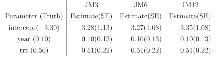
needed to be estimated. In addition, the joint-modeling approach is able to accurately

estimate ﬁxed eﬀects in the R-model, which other models do not provide. Results from the

JM approach are presented in Table 2.4. Obviously, the joint-model approach provides

accurate estimates regardless how many number of patterns are speciﬁed in the model

(34)

FA JM3 JM6 JM12 SP 0.00 0.02 0.04 0.06 0.08 age

FA JM3 JM6 JM12 SP

0.6 0.8 1.0 1.2 1.4 1.6 bfs1

FA JM3 JM6 JM12 SP

1.4 1.6 1.8 2.0 2.2 2.4 bfs2

FA JM3 JM6 JM12 SP

0.4

0.6

0.8

1.0

trt

FA JM3 JM6 JM12 SP

−0.8

−0.6

−0.4

−0.2

tscore

FA JM3 JM6 JM12 SP

0.2 0.3 0.4 0.5 0.6 0.7 0.8 year

Figure 2.2: Parameter estimates of fixed effects in the Y-model from joint-modeling approach with different patterns under Scenario 1.

Table 2.3: Comparison of two versions ofDIC’s. DIC1 (Spiegellhalter et al., 2002) and

DIC2 (Gelman et al., 2003).

JM3 JM6 JM12 SP

DIC1 89.4% 9.2% 1.4% 0%

(35)

Table 2.4: Comparison of estimates and their SE’s for ﬁxed eﬀects in the R-model from joint-modeling approach based on the scenario 1

JM3 JM6 JM12

Parameter (Truth) Estimate(SE) Estimate(SE) Estimate(SE)

intercept(−3.30) −3.28(1.13) −3.27(1.08) −3.35(1.08)

year (0.10) 0.10(0.13) 0.10(0.13) 0.10(0.13)

trt (0.50) 0.51(0.22) 0.51(0.22) 0.51(0.22)

2.3.2

Results Based on Scenario 2

In the second scenario, R_ij’s are allowed to depend on responses and treatments and

are generated by the following model,

R_ij ∼Ber(π_ij)

logit(π_ij) = α₀+α₁trt_i+α₂Y_ij +α₃year_i (2.21)

where (α₀, α₁, α₂) = (−3,0.8,1.2,0.1). Again on the average about 16% of data are

missing. Notice that the true model generating the data in this scenario does not belong

to the class of models considered by JM and PI approaches. Moreover, unlike in the ﬁrst

scenario, the true number of missing patterns is no longer known.

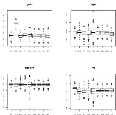
The simulation results based on Scenario 2 are shown in Figure 2.3, in which 4 ﬁxed

effects are presented and there are no big difference among all models for the rest of fixed

eﬀects. As expected, the LOCF approach produces highly biased estimates. Comparing

the PI approach and the JM method, we are able to see the same trend as in ﬁrst

scenario. Estimates of the PI approach ﬂuctuate as the number of patterns varies. The

JM approach provides stable estimates regardless of the number of patterns posited

in the model. Overall, estimates obtained from the PI method have more variations

than those from the JM approach. The SP model has the similar performance as the

JM model except that its parameter estimate for the variable“age” is more biased. As

expected, estimates of the treatment eﬀects are moderately biased. However, the JM

(36)

approach reduces the bias by about 31% as compared to the estimate based on the

full-data analysis. Except the treatment eﬀect, the JM approach appears to provide

unbiased estimates for other ﬁxed eﬀects despite the fact that the assumed model is not

correct. Hence, the JM approach is preferred over the PI method. With respect to model

selection, again both deﬁnitions of DIC’s have the similar preference. On average, the

JM approach with 3 patterns are selected 71.6%, 18.8% for 6 patterns, and 9.6% for 12

patterns. Therefore, the JM approach with 3 patterns might be the best model for this

(37)

FA LOCF PI3 PI6 PI12 JM3 JM6 JM12 SP

0.2

0.4

0.6

0.8

1.0

1.2

year

FA LOCF PI3 PI6 PI12 JM3 JM6 JM12 SP

0.00

0.05

0.10

0.15

age

−2.5

−2.0

−1.5

−1.0

−0.5

0.0

tscore

−0.5

0.0

0.5

1.0

1.5

trt

(38)

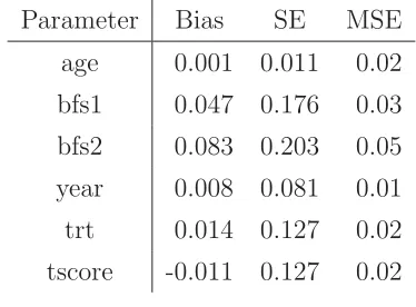
Table 2.5: Results of simulation for the joint modeling with the misspeciﬁcation of the

distribution for random patterns.

Parameter Bias SE MSE

age 0.001 0.011 0.02

bfs1 0.047 0.176 0.03

bfs2 0.083 0.203 0.05

year 0.008 0.081 0.01

trt 0.014 0.127 0.02

tscore -0.011 0.127 0.02

2.3.3

Sensitivity Analysis for the JM Approach

Notice that it is assumed the random patternuhas the bivariate normal distribution

in the JM approach and f(R|X, u) follows a logistic-regression model. In this section,

sensitivity of the model will be assessed on these two respects.

First, we use the same model as the one in Scenario 1 with three patterns but u_i is

generated by a mixture of two normal distributions given by N(µ₁,Σ₁) and N(µ₂,Σ₂)

with weights 2/3 and 1/3, respectively, where µ₁ = (−1.5,0)T, µ₂ = (1.5,0)T, Σ₁ = 1,

and Σ₂ = 3.06

For this scenario about 11.5% of data are missing. After data are generated, we ﬁt

the JM with 3 patterns. The biases, standard errors (SE’s), and MSE’s of parameter

estimates are reported in Table 2.5. None of these biases is substantially large (≤ 5%).

Both SE’s and MSE’s are fairly small. Hence, the JM approach provides consistent

estimates of fixed effects in the Y-model even though the distribution of random effects

is misspeciﬁed.

Second, we use the data simulated in Scenarios 1 with 3 patterns and ﬁt the same

Y-model but a probit regression for the R-model instead of the logistical regression used

for data generation. In other words, the assumed R-model is not correct. Here, we only

consider 3 patterns in the simulation. Results are summarized in Figure 2.4. Apparently,

(39)

by the JM with a probit regression are slightly larger. Therefore, the JM generally

delivers robust estimates even when the model for the missing indicators are not correctly

postulated.

2.4

Conclusions

We proposed two approaches, the pseudo-imputation method and the joint-modeling

method, that are general enough in the sense that both methods can be applied to

contin-uous and discrete outcomes. Here, we assumed that a surrogate variable can be correctly

identiﬁed. Based on our simulation studies, we see that the LOCF approach provides

bi-ased estimates even when the missingness is not informative. The PI method performed

well only if the missingness depends on missing patterns and the underlying number of

patterns is correctly speciﬁed. When the number of patterns is incorrectly deﬁned, the

PI method produces biased estimates. On the other hand, the JM method gives

approxi-mately unbiased estimates as long as the the missing depends on patterns even when the

number of patterns is not correctly speciﬁed. The SP model performs similarly in overall

as the JM model although it seems to produce comparatively more based estimates. In

cases of the missingness depending on the unobserved responses themselves, all methods

provide biased estimates but the JM based method reduces the bias substantially for the

estimate of the treatment eﬀect. In terms of model selection, the DIC criteria picks the

right model about 90% for the joint-modeling approach. Furthermore, the JM approach

is not sensitive to mild model violations. Overall, the joint model approach is preferred.

In the cases of absence of a surrogate variable, patterns may be deﬁned according

to available covariates but extreme care must be given since misspeciﬁcation of patterns

may introduce serious bias and produce misleading conclusions. This issue is explained

(40)

JM_L JM_P 0.02 0.04 0.06 0.08 age JM_L JM_P 0.6 0.8 1.0 1.2 1.4 1.6 bfs1 JM_L JM_P 1.4 1.6 1.8 2.0 2.2 2.4 bfs2 JM_L JM_P 0.4 0.6 0.8 1.0 trt JM_L JM_P −0.8 −0.6 −0.4 −0.2 tscore JM_L JM_P 0.2 0.3 0.4 0.5 0.6 0.7 year

(41)

Chapter 3

Modeling NIM Data using GAM

A parametric generalized linear model may not be appropriate especially when some

measurements are non-ignorable missing. Also a speciﬁc parametric structure can not be

validated easily. Such parametric structures may lead to possible bias when the

under-lying model for the full data is nonlinear. Particularly, the generalized linear model used

in the ﬁrst step for the PI approach may not produce reliable estimates of the predictive

means that will be used in latter steps. Therefore, ﬁnal estimates might be biased and

inference will be misleading. Hence, instead of the generalized linear model, we consider

the use of the generalized additive model (GAM) proposed by Hastie and Tibshirani

(1990). As it is known, parameters in GAM can be diﬃcult to interpret. However,

para-meters need not to be interpretable in the ﬁrst step of the PI approach and hence we can

still apply GAM to obtain the predictive means for latter use. Moreover, in situations

that only the treatment eﬀect or eﬀects of other discrete covariates may be of primary

interest, estimations in terms of odds ratios can be obtained without much trouble. A

brief description about generalized additive models and model ﬁtting techniques is given

in Section 3.1. Section 3.2 provides simulation results comparing a generalized linear

model and a generalized additive model within the PI method. Possibilities of ﬁtting the

(42)

3.1

Model Description

Many nonparametric methods do not perform well when there is a large number of

independent variables in the model. The sparseness of data in this setting inﬂates the

variance of the estimates. The problem of rapidly increasing variance for increasing

di-mensionality is sometimes referred to as the curse of didi-mensionality . To overcome this

diﬃculty, Stone (1985) proposed additive models. These models estimate an additive

approximation to the multivariate regression function. The beneﬁts of an additive

ap-proximation are at least twofold. First, since each of the individual additive terms is

estimated using a univariate smoother, the curse of dimensionality is avoided, at the

cost of not being able to approximate universally. Second, estimates of the individual

terms explain how the dependent variable changes with the corresponding independent

variables.

Hastie and Tibshirani (1990) proposed generalized additive models that extend the

traditional additive models (Stone, 1985) to accommodate more distribution functions.

These models assume that the mean of the dependent variable depends on an additive

predictor through a nonlinear link function. Generalized additive models permit the

response probability distribution to be any member of the exponential family of

dis-tributions. Many widely used statistical models belong to this general class, including

additive models for Gaussian data, nonparametric logistic models for binary data, and

nonparametric log-linear models for Poisson data.

The generalized additive models can be expressed as

E(Y_i|X_i) =g(s₀+

p

i=1

s_i(X_i)) (3.1)

where g(·) is a known link function, s_i(·)’s are smooth functions, and pis the number of

the predictor variables. The GAM can also be used to incorporate partial linear models

(Hastie and Tibshirani, 1986). This is achieved by replacing some smooth functions with

linear functions. Thus, parameters in linear functions in the GAM can be interpretable,

which makes it possible to draw inferences for some covariates if they are of primary

(43)

The estimating procedure for generalized additive models consists of two loops. The

local scoring algorithm is used in the outer loop and a weighted backﬁtting algorithm for

the inner loop. The local scoring algorithm uses a modiﬁed form of adjusted dependent

variable regression, as described for generalized linear models in McCullagh and Nelder

(1989), with the additive predictor taking the role of the linear predictor (Hastie and

Tibshirani, 1986). The backﬁtting algorithm (Friedman and Stuetzle, 1981; Hastie and

Tibshirani, 1986) is a general algorithm for an additive model using any

regression-type ﬁtting mechanisms. This algorithm always converges for Gaussian distribution

(Hastie and Tibshirani, 1986). However, for other distributions, numerical instabilities

with weights may cause convergence problems. Even when the algorithm converges, the

individual functions need not be unique, since dependence among the covariates can

lead to more than one representation for the same ﬁtted surface. A weighted backﬁtting

algorithm has the same form as for the un-weighted case, except that the smoothers

are weighted according to distribution functions. Both PROC GAM in SAS/STAT and

GAM in R package of MGCV can be used to ﬁt these models.

3.2

Simulation Studies

The objective of the ﬁrst simulation is to compare the performance of diﬀerent models

used at the ﬁrst step in the PI method. The model used in the Chapter 2 is a generalized

linear model (GLM) and we also use a generalized additive model (GAM) in this

sim-ulation. For simplicity, these two strategies are referred to as the PI-GLM method and

the PI-GAM method. At the second stage, we will still use a generalized linear model

as described in Chapter 2. Data are generated by using the same models described in

Chapter 2 under Scenario 1. The underlying Y-model follows a logistic regression and

the missing indicator depends on missing patterns. One thousand Monte Carlo samples

are simulated and the sample size for each sample is 1800.

Simulation results are summarized in Figures 3.1 − 3.3. When the conﬁguration

of patterns is correctly known, both models yield precise estimates. When patterns

are misspeciﬁed, the PI-GAM method provides slightly more biased estimates than the

(44)

than estimates from the PI-GLM method. Thus, the methods appear to be approximately

unbiased. Also from the boxplots in Figure 3.1, we see that the sampling distributions of

the parameter estimates are very similar. Overall, the PI-GLM method and the PI-GAM

method have the similar performance in terms of parameter estimation. Hence, there is

no significant loss of efficiency to fit a GAM at the first step of the PI method even when

the underlying Y-model is a GLM.

In the second simulation study, the full data are generated from the following model

Y_i ∼Ber(p_i)

logit(p_i) =β₀+β₁trt_i +f(age_i) (3.2)

where βT = (β₀, β₁) = (−1.5,0.3) are true values of parameters and

f(age) = 0.001(age−20)(age−30)(age−40)I(age<40) + 0.1(age−40)I(age>40). The

values of age for each individual are generated from U nif orm(18,58). The surrogate

variable W_i = 0.7×logit(p_i) +e_i, where e_i ∼ N(0,0.82). Patterns are determined in the

same way as in Chapter 2.

Notice that the model used to generate data in this simulation is determined according

to the real data from the AIDS study which we will analyze in the last chapter. To

simplify the simulation, we only include two independent variables, treatment (trt) and

age in the model. The treatment variable is binary and the age variable is continuous.

The curve of the spline function versus the corresponding covariate is given in Figure 3.4.

Obviously, the relation with age is non-linear.

Then, the missing indicator R_i is generated using the following model:

R_ij ∼Ber(π_ij)

logit(π_ij) =α₀+α₁ ∗trt_i+Z_iu_i (3.3)

where trt_i, a subvector of X_i, denotes the treatment assignment, (α₀, α₁) = (−3,1.7),

and u_i ∼ N(0,0.752). On average, 15% of data were found to be missing.

As in the ﬁrst simulation, a total of one thousand Monte Carlo samples are

(45)

method and the PI-GAM method to fit to each dataset. Difference from the first

sim-ulation is that we also ﬁt the GLM and the GAM accordingly at the second stage. A

summary of results is presented in Figure 3.5. It is clear from Figure 3.5 that the PI-GAM

method provides more accurate estimates compared to the PI-GLM method.

In summary, the PI method with the GAM has similar performance even when the

un-derlying Y-model follows a generalized linear model. Moreover, it yields precise estimates

when the underlying Y-model is nonlinear. Hence, the PI-GAM method is preferred

uni-versally. In practice, the underlying distribution is unknown and missing data adds more

uncertainty. A good strategy would be to obtain the predictive mean by ﬁtting a GAM

at the ﬁrst stage of the PI method. Then plot the predictive mean versus covariates to

discover the potential data structure and ﬁt the model accordingly. When the treatment

eﬀect is of primary interest, we can ﬁt the GAM within the PI method at both stages.

3.3

The JM Approach with GAM

It has been shown via simulation studies presented in Chapter 2 that the JM approach

performs better than other approaches. As the treatment eﬀect is of primary interest,

one may prefer to adopt the JM approach with the GAM in the Y-model (Equation 2.8)

over the PI method. However, it is generally diﬃcult, at least for practical statisticians,

to ﬁt smooth functions within Bayesian framework since there is no existing program or

procedure available to resolve this task in r

Analyzing Longitudinal Data with Non-ignorable Missing

LIANSHENG ZHU

Acknowledgements

Contents

List of Tables

List of Figures

Chapter 1

A Motivating Study

Notations and Definitions

Models and Associated Methods for NIM Data

Selection Models

Pattern-mixture Models

Chapter 2

The Pseudo-imputation (PI) Method

Example

Extension and Asymptotic Property

Joint Modeling

Prior Selection and Posterior Computation

Model Selection

Simulation Study

Results based on Scenario 1

FA LOCF PI3 JM3

tscore

Results Based on Scenario 2

FA LOCF PI3 PI6 PI12 JM3 JM6 JM12 SP

Sensitivity Analysis for the JM Approach

Conclusions

Chapter 3

Model Description

Simulation Studies

The JM Approach with GAM