XIA, MENG. Cape Fear River Estuary Modeling System. (Under the direction of Dr. LIAN XIE).
The Cape Fear River Estuary (CFRE) region is one of the coastal regions facing frequent threats from tropical cyclones. It is also an important nursery for juvenile fish, crabs, shrimp, and other biological species. Thus, predicting the physical responses of the CFRE system to extreme weather events is important to the protection of life and property and ensuring the economical well beings of local residents. In this study, the Princeton Ocean Model (POM) is used to simulate the storm surge circulation in the CFRE and adjacent Long Bay and Onslow Bay.
The Environmental Fluid Dynamic Code (EFDC), an estuarine and coastal ocean circulation model, is also used to simulate the salinity plume and tracer plume distribution and particle trajectory in the vicinity of the mouth of the Cape Fear River Estuary (CFRE). The effects of astronomical tide, river discharge and wind on the CFRE salinity plume and tracer plume, particle trajectory were investigated. The comparison among the plume structure, particle trajectory, and the passive tracer structure is discussed.
Cape Fear River Estuary Modeling System
By
Meng Xia
A dissertation submitted to the Graduate Faculty of North Carolina State University
In partial fulfillment of the Requirements for the degree of
Doctor of Philosophy
Marine, Earth and Atmospheric Sciences
Raleigh, NC Dec, 2006 Approved by:
Dr. Leonard J. Pietrafesa Dr. John M. Morrison
Dr. Daniel L. Kamykowski Dr. Lian Xie
DEDICATION
Special thanks to my wife and my parents. Without their love, encouragement and support, I couldn’t have completed this dissertation and faced this challenge.
BIOGRAPHY
I wish to thank Dr. Lian Xie, the chair of the advisory committee, for his guidance, support and encouragement on this research. I appreciate that Dr. Xie provides me a very flexible research environment that is suitable for my research interests and strength. I always have freedom to explore some new ideas with available resources. I also benefit a lot from his methodology in ocean numerical modeling, his many thoughtful ideas that keep my research topic in step with current active research in this area.
I want to express my appreciation to the advisory committee members, Dr. Leonard Pietrafesa, Dr. John Morrison and Dr. Daniel Kamykowski for their support, thoughtful input and advice on this research. They are also very helpful in providing me with various resources for the study. Thanks to all the friends in the Coastal Fluid Dynamics Lab.
Table of Contents
List of Tables ···vii
List of Figures ···vii
Chapter 1. Introduction···1
Chapter 2. Cape Fear River Estuary Storm surge Modeling···6
1. Introduction···7
2. Model configuration of the Cape Fear River Estuary System ···9
3.Winds and experimental settings···11
4. Results ···13
5.Model Verification···18
6.Discussion and Conclusions···18
References···22
The list of the table captions···25
The list of the figure captions···25
Tables ···27
Figures ···30
Chapter 3. Cape Fear River Estuary Plume Modeling···44
1. Introduction···45
2. Model description and configuration···47
3. The plume case studies of March 22, 2005···51
4. Sensitivity Experiments···52
5. Summary and conclusions ···60
References ···63
The list of the figure captions···69
Figures···71
Chapter 4. Modeling Cape Fear River Estuary Plumes: A Sensitivity Study to Model Settings···85
1. Introduction···86
4. Results ···89
5. Discussion and conclusions ···94
References···95
The list of the figure captions···99
Figures···100
Chapter 5. A Numerical Study of Passive Tracer and Particle Trajectories in the Cape Fear River Estuary ···108
1. Introduction···109
2. Model description and configuration···110
3. Model Settings···111
4. Result···111
5. The comparison of the results to plume modeling···116
6. Summary and conclusions···119
References···121
The list of the figure captions ···123
Figures···125
Chapter 6. Final Remarks···153
L
ist of tables:
Table 1. Dates and corresponding intensities of the Hurricanes···27
Table 2. The time, location and pressure of hurricane Fran (1996) ···27
Table 3. The time, location and pressure of Hurricane Bertha (1996) ···28
Table 4. The time, location and pressure of Hurricane Floyd (1999) ···29
Table 5. The time, location and pressure of Hurricane Charley (2004) ···29
List of figures:
Chapter2:
Figure 1. The location of Cape Fear River Estuary and adjacent coastal area···30Figure 2. The land relief and bathymetry of the Cape Fear Estuary System···31
Figure 3. The tracks of four hurricanes which passed by the CFRE region···32
Figure 4. Wind distribution at 09/05/2100Z, 09/05/2300Z, 09/06/0100Z, 09/06/0300Z as Hurricane Fran made landfall in the Cape Fear region···33
Figure 5. Wind Distribution at 07/12/1700Z, 07/12/1900Z, 07/12/2100Z, 07/12/2300Z as Hurricane Bertha passed by the Cape Fear region···34
Figure 6. Wind distribution at 09/16/0500Z, 09/16/0700Z, 09/16/0900Z, 09/16/1100Z as Hurricane Floyd passed by the Cape Fear region···35
Figure 7. Wind distributions at 08/14/1400Z, 08/14/1500Z, 08/14/1600Z, 08/14/1700Z as Hurricane Charley brushes the Cape Fear region···36
Figure 8. Simulation of storm surge (m) and inundation at 09/05/2100Z, 09/05/2300Z, 09/06/0100Z, 09/06/0300Z for Hurricane Fran···37
Figure 9. Simulation of storm surge (m) and inundation at 07/12/1700Z, 07/12/1900Z, 07/12/2100Z, 07/12/2300Z for Hurricane Bertha···38
Figure 12. The comparison of model data and water level observation in Hurricane Bertha (From left to Right: Yaupon Beach, NC, Wilmington, NC, Lenoxville Point, NC,
Morehead City Harbor, NC, Beaufort, NC, Duck Pier, NC) ···41
Figure 13. The comparison of model data and water level observation in Hurricane Fran (From left to Right: Springmaid Pier, SC, Yaupon Beach, NC, Wilmington, NC, Beaufort (Taylor Creek ), NC,Morehead City Harbor, NC.) ···41
Figure 14. The comparison of model data and water level observation in Hurricane Floyd (From left to Right: Army Depot, SC, Wilmington, NC, Beaufort, NC, Cape Hatteras Fishing Pier, NC, Duck Pier , NC. ) ···42
Figure 15. The comparison of model data and water level observation in Hurricane Charley (From left to Right: Springmaid Pier, SC, Sunset Beach, NC, Wilmington, NC, Wrightsville Beach, NC, Beaufort, NC.) ···42
Figure 16. The comparison of modeled result and the observed water level···43
Chapter 3:
Figure 1. The location of the Cape Fear River Estuary···71Figure 2. The grids and bathymetry in the CFRE modeling domain···72
Figure 3. Comparison between model simulated and observed water level···73
Figure 4. Comparison between the simulated and observed salinity···74
Figure 5. The Sea surface salinity fields forced by normal river discharge···75
Figure 6. The vertical salinity fields forced by normal river discharge···75
Figure 7. Surface salinity fields forced by 5m/s winds and normal discharge···76
Figure 8. Vertical salinity fields forced by 5 m/s winds and normal discharge···76
Figure 9. Surface plume structure under southwesterly winds and normal river discharge: Response to 20 m/s wind speed···77
Figure 10.Vertical plume structure under southwesterly winds and normal river discharge: Response to 20 m/s wind speed···77
Figure 11. Surface plume structure with southwesterly winds of 5m/s: (a) Response to no river discharge (b) Response to flood conditions···78 Figure 12. Vertical plume structure with southwesterly winds of 5m/s: (a) Response to no river discharge (b) Response to the flood condition···78 Figure 13. Surface Plume structure with no wind forcing and normal discharge: (a) Response to low water level condition (b) Response to high water level condition···79 Figure 14. Vertical Plume structure with no wind forcing and normal discharge: (a) Response to low water level condition (b) Response to normal condition after low tide (c) Response to high water level condition (d) Response to normal condition after the high tide···80 Figure 15. Surface Plume structure with southwest wind forcing and normal discharge: (a) Response to low water level condition (b) Response to high water level condition···81 Figure 16. Vertical Plume structure with southwest wind forcing and normal discharge: (a) Response to low water level condition (b) Response to normal condition after low tide (c) Response to high water level condition (d) Response to normal condition after high tide···82 Figure 17. Surface salinity fields forced by 5m/s winds and normal discharge (a) Response to northerly winds (b) Response to northwesterly winds···83 Figure 18. The plume type under the different physical settings···84
Chapter 4:
Figure 1. The location of Cape Fear River Estuary and adjacent coastal area···100
Figure 2. The grids of the CFRE modeling (a) Grid 1 of the model domain (b) Grid 2 of the model domain···101
Figure 3. Simulation under the normal river discharge and upwind advection scheme (a) Surface plume structure (b) Bottom plume structure···101
Figure 7. Simulation under the normal river discharge and central difference advection scheme (a) Surface plume structure (b) Bottom plume structure···103 Figure 8. Simulation under the normal river discharge and Smolar-2 advection scheme (a) Surface plume structure (b) Bottom plume structure···104
Figure 9. Simulation under 4 layer resolution and Smolar-2 advection scheme (a) Surface plume structure (b) Bottom plume structure···104
Figure 10. Simulation under 6 layer resolution and Smolar-2 advection scheme (a) Surface plume structure (b) Bottom plume structure···105
Figure 11. Simulation under 11 layer resolution and Smolar-2 advection scheme (a) Surface plume structure (b) Bottom plume structure···105
Figure 12. Simulation under 10 layer resolution and Smolar-2 advection scheme (a) Surface plume structure (b) Bottom plume structure···106
Figure 13. Simulation under 12 layer resolution and Smolar-2 advection scheme (a) Surface plume structure (b) Bottom plume structure···106
Figure 14. Simulation under 11 layer resolution and Smolar-2 advection scheme (a)Simulation under the grid 2 (b) Simulation under the grid 1···107
Chapter 5:
Figure 1. The location of the Cape Fear River Estuary···125
Figure 2. The grids and bathymetry in the CFRE modeling domain. (a) The grid of the model domain (b) The bathymetry of the model domain···126 Figure 3. The sea traces fields forced by normal river discharge. (a) The surface tracer structure after 5 days (b) The tracer vertical structure after 5 days···127 Figure 4. Sea surface traces fields forced by 5 m/s winds and normal discharge (a) Response to northerly winds (b) Response to northeasterly winds (c) Response to easterly winds (d) Response to southeasterly winds (e) Response to southerly winds (f) Response to southwesterly winds (g) Response to westerly winds (h) Response to northwesterly winds···128 Figure 5. Vertical tracer fields forced by 5 m/s winds and normal discharge (a) Response to northerly winds (b) Response to northeasterly winds (c) Response to easterly winds (d)
Response to southeasterly winds (e) Response to southerly winds (f) Response to southwesterly winds (g) Response to westerly winds (h) Response to northwesterly winds···132 Figure 6. Sea surface traces fields under northeasterly winds and normal river discharge (a) Response to 5 m/s wind speed (b) Response to 10 m/s wind speed (c) Response to 15 m/s wind speed (d) Response to 20 m/s wind speed···134 Figure 7. Tracer structure under southwesterly winds and normal river discharge (a) Response to 5 m/s wind speed (b) Response to 10 m/s wind speed (c) Response to 15 m/s wind speed (d) Response to 20 m/s wind speed···136 Figure 8. Tracer structure under northeasterly winds and normal river discharge (a) Response to 5 m/s wind speed (b) Response to 10 m/s wind speed (c) Response to 15 m/s wind speed (d) Response to 20 m/s wind speed···138 Figure 9. Tracer structure under southwesterly winds and normal river discharge (a) Response to 5 m/s wind speed (b) Response to 10 m/s wind speed (c) Response to 15 m/s wind speed (d) Response to 20 m/s wind speed···139 Figure 10. Tracer structure with southwesterly winds of 5m/s (a) Response to no river discharge (b) Response to normal river discharge c) Response to 1.5 times normal river discharge (d) Response to flood conditions···140 Figure 11. Tracer structure with southwesterly winds of 5m/s (a) Response to no river discharge (b) Response to normal river discharge c) Response to 1.5 times normal river discharge (d) Response to flood conditions···142 Figure 12. Tracer structure with no wind forcing and normal discharge (a) The structure at low tide (b) The structure at high tide···143 Figure 13. Tracer structure with no wind forcing and normal discharge (a) Response to low tide condition (b) Response to normal condition after low tide (c) Response to high tide condition (d) Response to normal condition after high tide···144 Figure 14. Tracer structure with southwest wind forcing and normal discharge (a) The structure at low tide (b) The structure at high tide···145 Figure 15. Tracer structure with southwest wind forcing and normal discharge
(a) Response to low tide condition (b) Response to normal condition after low tide (c) Response to high tide condition (d) Response to normal condition after high tide···146
xii
Chapter 1. Introduction
1.
Scientific Background
The Cape Fear River, a 322 km river that flows through the heart of the North Carolina (NC)
piedmont, has the largest watershed in NC. Originally known as the Waccamaw, the Cape
Fear is the largest river basin in NC and the only one that flows directly into the ocean. The
Black River joins the Cape Fear 24 km above Wilmington, and the Northeast Cape Fear
River enters the system at Wilmington. The freshwater discharge from the Cape Fear River,
the Northeast Cape Fear River, and the Black River converges in the Cape Fear Estuary and
then flows into Long Bay (Figure 1). The average combined discharge from these rivers is
about 221 m3/s (Dame et al., 2000), with a maximum of about 2000 m3 /s.
The head of the CFRE connects to the eastern end of Long Bay on the Atlantic seaboard.
Because of the in-welling of coastal waters into the estuary due to the combined effects of
the astronomical tides and wind forcing (Pietrafesa and Janowitz, 1988), this region is an
extremely important nursery for juvenile fish, crabs, and shrimp (Miller et al., 1984). The
Cape Fear River is the only coastal river system in NC where hybrid striped bass are stocked
(Patrick and Moser, 2001).
The plume associated with the CFRE system is an interesting phenomenon of the east coast
of the United States. Plumes from the CFRE reduce salinity and change other water
properties in the coastal waters, such as temperature, nutrients, and phytoplankton. The
al., 2005).
The CFRE also experiences significant cycling of nutrients (Norris and Hackney, 1999) and
heavy metals (Shank et al., 2004). Hurricane-induced storm surge circulation could influence
sediment and nutrient transport in the river and estuary (Wren and Leonard 2005, Sheremet
et al. 2005, Leonard et al. 1995, Nyman et al. 1995). A major storm surge may also impact
Dissolved Oxygen which could deleteriously impact living marine resources (Mallin et al.,
1999). Hurricane wind induced storm surge and inundation could bring sewage runoff into
the river, an environment-damaging impact to the CFRE region. This is especially the case
near the mouth of the estuary.
The Cape Fear has faced several threats from tropical and extra-tropical cyclones since 1996.
The Cape Fear and adjacent Long Bay seem to have been a magnet for hurricanes. Usually
these tropical cyclones invade the region in the late summer and early fall, such as the Fran
(Sep, 1996), Bertha (July, 1996), Bonnie (Aug, 1998), and Floyd (Sep, 1999). Hurricane
Charley visited the Cape Fear in August, 2004 after several quiet years in the region.
2. Purpose of the Study
In this study, the Princeton Ocean Model (POM) will be used to simulate the
hurricane-induced storm surge, and the Environmental Fluid Dynamics Code (EFDC) will be used to
study salinity and trace plume distribution and the particle trajectories at the CFRE and
adjacent coastal region.
Specially, the proposed study will address the following questions:
1) What is the influence of Hurricane track and intensity to the storm surge
distribution?
2) What is the effect of Frying Pan Shoals, between Long Bay and Onslow Bay to the
storm surge circulation and plume distribution?
3) What is the plume horizontal and vertical structure under different wind forcing, river
discharge effect, tidal effect? And what is the possible reason for the transition?
4) What is the best modeling setting to simulate the plume structure? Such as vertical
resolution, horizontal resolution, advection scheme?
5) What are the horizontal and vertical structures of passive tracer plumes and the path
of particle trajectories under different wind forcing, river discharge effect, tidal
effect? What are the possible causes for the differences and similarities?
3. Organization of dissertation
A numerical study of storm surge in the Cape Fear River Estuary and adjacent coastal waters
are given in chapter 2. Chapter 3 introduces numerical modeling of Cape Fear River Estuary
plumes. A sensitivity study of model settings for modeling the Cape Fear River Estuary
plumes is investigated in Chapter 4. A numerical study of passive tracer and particle
trajectories in the Cape Fear River Estuary are presented in Chapter 5. Finally, Chapter 6
Dame, R., Alber, M., Allen, D., Mallin, M., Montague, C., Lewitus, A., Chalmers, A.,
Gardner, R., Gilman, C., Kjerfve, B., Pinckney, J., Smith, N. (2000) “Estuaries of the South
Atlantic Coast of North America: Their Geographical Signatures” Estuaries 23, 793–819.
Leonard, A. L., Hine, C. A., Luther, E. M., Stumpf, P. R., and Wright, E. E. (1995),
Sediment transport processes in a west-central Florida open marine marsh tidal creek: The
role of tides and extra-tropical storms. Estuarine,Coastal and Shelf Science, 41, 225-248.
Mallin, M. A., Posey, M. H, Shank, G. C, Mciver, M. R, Ensign, S. H, and Alphin, T. D.
(1999), Hurricane effects on water quality and benthos in the cape fear watershed: Natural
and anthropogenic impacts. Ecological Applications, 9, 350-362.
Miller, J.M.; Reed, J.P., and Pietrafesa, L.J., (1984), Patterns, mechanisms and approaches to the study of migrations of Estuarine-dependent fish larvae and juveniles. Mechanisms of migration in: Fishes. McCleave, J.D.; Arnold, G.P.; Dodson,J.J., and Neill, W.H (eds.), New York: Plenum, 209-225
Nyman, J. A., Crozier, C. R., and DeLaune, R. D. (1995), Roles and patterns of hurricane
sedimentation in an Estuarine Marsh. Estuarine,Coastal and Shelf Science, 40, 665-679.
Patrick, S. W., and Moser, L. M. (2001), Potential competition between Hybrid Striped Bass (Morone saxatilis X M. americana) and Striped Bass (M. saxatilis) in the Cape Fear River Estuary, North Carolina. Estuaries, 24, 425-429.
Pietrafesa, L.J., Janowitz, G.S., (1988) Physical Oceanographic Processes Affecting Larval Transport Around and Through North Carolina Inlets. American Fisheries Society, 3, 34-50
Shank, G. C., Skrabal, A.S., Whitehead, F. R., and Kieber, J. R. (2004), Fluxes of strong Cu-complexing ligands from sediments of an organic-rich estuary. Estuarine, Coastal and Shelf Science, 60, 349-358.
Sheremet, A., Mehta, J.A., Liu, B., and Stone, W.G. (2005), Wave–sediment interaction on a
muddy inner shelf during Hurricane Claudette. Estuarine,Coastal and Shelf Science, 63 ,
225-233
Wren, P. A., and Leonard, L.A. (2005), Sediment transport on the mid-continental shelf in
Onslow Bay, North Carolina during Hurricane Isabel. Estuarine,Coastal and Shelf Science,
Fear River Estuary and Adjacent Coast
Abstract
The Cape Fear River Estuary (CFRE) region is one of the coastal regions facing frequent
threats from tropical cyclones. It is also an important nursery for juvenile fish, crabs, shrimp,
and other biological species. Thus, predicting the physical responses of the CFRE system to
extreme weather events is important to the protection of life and property and ensuring the
economical well-beings of local residents. In this study, the Princeton Ocean Model (POM)
was used to simulate the storm surge, inundation, and coastal circulation in the CFRE and its
adjacent Long Bay using a three-level nesting approach. Hindcasts of the hydrodynamic
responses of the CFRE system to historic events were performed for Hurricanes Fran, Floyd,
Bertha and Charley. Comparisons were made for the modeling results and the observations.
1. Introduction
The Cape Fear River, a 322 km river that flows through the heart of the North Carolina (NC)
piedmont, has the largest watershed in NC. Originally known as the Waccamaw, the Cape
Fear is the largest river basin in NC and the only one that flows directly into the ocean. The
river begins near Greensboro and Winston-Salem as two rivers, the Deep River and the Haw
River. These two rivers converge near Moncure to form the Cape Fear River. The Black
River joins the Cape Fear 24 km above Wilmington, and the Northeast Cape Fear River
enters the system at Wilmington (Figure 1). The Cape Fear River basin covers 23,310 km
and encompasses streams in 29 of the state's 100 counties.
2
The mouth of the CFRE connects the eastern end of Long Bay on the Atlantic seaboard.
Because of the in-welling of coastal waters into the estuary due to the combined effects of
the astronomical tides and wind forcing (Pietrafesa and Janowitz, 1988), this region is an
extremely important nursery for juvenile fish, crabs, and shrimp (Miller et al., 1984). The
Cape Fear River is the only coastal river system in NC where hybrid striped bass are stocked
(Patrick and Moser, 2001). In addition, it is an important natural resource that facilitates
industry, transportation, recreation, drinking water, and aesthetic enjoyment.
The CFRE experiences significant cycling of nutrients (Norris and Hackney, 1999) and
heavy metals (Shank et al.., 2004). Hurricane-induced storm surge circulation could
impact Dissolved Oxygen which could deleteriously impact living marine resources (Mallin
et al., 1999). Hurricane wind induced storm surge and land inundation could bring sewage
runoff into the river, an environment-damaging impact to the CFRE region. This is especially
the case near the mouth of the estuary.
The CFRE has recently experienced the passage of a large number of tropical and
extra-tropical cyclones since 1996. Usually these extra-tropical cyclones invaded the region in late
summer and early fall, such as Bertha (July, 1996), Fran (September, 1996), Bonnie (August,
1998), Dennis (September, 1999), Floyd (September, 1999), Irene (October, 1999), Charley
(August, 2004) and Ophelia (August, 2005). In this study, storm surge and coastal ocean
circulation hindcasts are performed for Hurricanes Bertha, Fran, Floyd and Charley since
these Hurricanes greatly influenced the CFRE and its adjacent ocean. Their landfall dates and
corresponding intensities are listed in Table 1.
Following the earlier model work of Pietrafesa et al. (1997), Peng (2002), Xie et al. (2004)
and Peng et al. (2004) in the Croatan-Albemarle-Pamlico Estuary System (CAPES), we will
use a three-dimensional storm surge model to simulate hurricane-induced storm surge and
land inundation in the CFRE system. In section 2, the storm surge model is briefly described.
The method used to compute the hurricane winds is presented in section 3. Main results are
presented in section 4, and model validation is performed in section 5, followed by
discussions and conclusions in section 6.
2. Model configuration of the Cape Fear River Estuary System
The storm surge model in Peng et al. (2004) is applied in this study. The hydrodynamics of
the model are based on the Princeton Ocean Model (Mellor, 1996), which is a sigma
coordinate model in that the vertical coordinate is scaled on the water column depth. The
horizontal grid uses curvilinear orthogonal coordinates and an "Arakawa C" differencing
scheme. The model contains an imbedded second moment turbulence closure sub-model to
provide vertical mixing coefficients. The horizontal time differencing is explicit, whereas the
vertical differencing is implicit. The latter eliminates time constraints for the vertical
coordinate and permits the use of fine vertical resolution in the surface and bottom boundary
layers. This model has a free surface and a split time step. The external mode portion of the
model is two-dimensional and uses a short time step based on the CFL condition and the
external gravity wave speed. The internal mode is three-dimensional and uses a long time
step based on the CFL condition and the internal wave speed. Complete thermodynamics
have been implemented.
The inundation scheme used in the CFRE model is a modified Hubbert and McInnes (1999)
scheme which we will refer to as the HM scheme. The HM scheme utilizes the vertically
averaged horizontal current as an inundation speed control. This modified scheme was
described in Xie et al. (2004) and Peng et al. (2004), hereafter referred to as the PXP scheme.
It employs the surface current as the inundation speed parameter. In order to determine if a
horizontal directions, x and , that the water could travel are computed through the time
step integral of the surface inundation speed at this grid point. The land grid point will be
flooded, or turned into a water point, if the water can travel over the corresponding grid size
along either x or y axis or both. Otherwise, the land grid point will remain dry.
y
The procedure for draining or drying in the PXP scheme also differs from the original HM
scheme. In the PXP scheme, draining occurs when the water depth goes below a preset
threshold. We also impose a mass balance constraint on the inundation process. An
interactive mass rebalancing procedure is implemented in both the flooding and draining
processes.
In this study, the storm surge and inundation modeling system is configured to the CFRE and
its adjacent shelf and coast (33.67 N-34.00 N, 78.25 W-77.75 W) (Figure 2). The
horizontal resolution is determined by a 90-m grid size in both the x and y directions, while
three sigma levels in the vertical were employed for adequacy and computational efficiency.
We used the bathymetry data which was derived from the National Geophysics Data Center
(NGDC) Coastal Relief Model Volume 02.
o o o o
The domain shown in Figure 2 is the inner domain of a three-level nesting system in the
study. The outer domain region is set between 32.50oN-36.50 N, 81.00 W- 75.00 W; the
middle domain is set between 33.17 N-34.50oN, 79.00 W- 77.17 W. The middle domain
bathymetry data was obtained from the NGDC Coastal Relief Model Volume 02 as well. For
o o o
o o o
the outer domain, ETOPO2 Global 2-Minute Gridded Elevation Data was used to couple
with the NGDC Coastal Relief Model Volume 02. This is because ETOPO2 contains the
deep ocean data necessary for the outer domain which are not covered by the NGDC
database. The bathymetry and elevation data are shown in Figure 2. A schematic depiction of
the nesting scheme is shown in Figure 3.
3. Winds and experimental settings
Several hurricanes passed over the CFRE domain since 1996. The tracks are presented in Fig
3.
The hurricane pressure field and surface wind velocity created by the pressure gradient were
modeled according to Holland (1980):
) / exp( ) ( B c n
c P P A r
P
P= + − − (1)
2 / 1 ] / ) / exp( ) (
[ B B
c n
c AB P P A r r
V = − − ρ (2)
where P is the atmosphere pressure at radius r; ρis the air density; is the central pressure
and is the ambient pressure (in practice, the value of the first anticyclonically curved
isobar); both A and B are scaling parameters; V is wind profile which results from the
hurricane pressure gradient. Those parameters are set to: , B=1.9, A= ;
is the radius of maximum wind and derived from the Hurricane Research Division
( c P /m n P c 3 2 . 1 kg =
ρ (R )B
max
max
R
The surface wind stress is computed through the following bulk formula:
w w
dV V
C v v
ρ
τ = (4)
where VW is the wind speed at height of 10m, and ρ is air density. The drag coefficient, Cd,
is assumed to vary with wind speed:
) 5 ( / 1 18 . 2 / 3 1 / 56 . 1 62 . 0 / 10 3 14 . 1 / 26 / 10 065 . 0 49 . 0 / 26 16 . 2 103 < < ≤ + < ≤ < ≤ + ≥ = s m V s m V V s m V s m V s m V s m V C w w w w w w w d
This Cd formula follows Large and Pond (1981) when the wind speed is less than 26m s-1,
otherwise, it is assumed as a constant as indicated in Powell et al. (2003).
Detailed information of the tracks and hurricane attributes are important for accurate surface
wind stress calculation. The time, location and central pressure of the specific hurricanes are
shown in tables 2-5. For example, the computation time for Hurricane Fran (1996) is from
09/05/15Z to 09/06/09Z based on the track, time, location, and pressure as shown in Table 2
and in Figure 3. The wind velocity distribution at different times is illustrated in Figures 4.
Similarly, the track, time, location and pressure information of hurricane Bertha (1996),
Floyd (1999), Charley (2004) are listed in Table 3, 4, 5 respectively. The corresponding wind
distributions are illustrated in Figure 5, 6, 7.
4. Results
4.1 Hurricane Fran (1996)
Hurricane Fran struck NC as a category three hurricane, and it swept across NC leaving a
swath of destruction throughout most of the state. Its track moved directly over the city of
Wilmington and Cape Fear Estuary, traveling north when it approached the CFRE and then a
little northwestward after that (Figure 3). Its best track position and pressure are given in
Table 2 and Figure 4.
From September 5 to September 6 in 1996, Hurricane Fran passed this region within 10
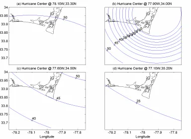
hours at a translation speed of 10 km/h. The simulated storm surge and inundation from
09/05/2100Z to 09/06/0300Z are shown every two hours in Figures 8 a-d. At 09/05/21Z, the
hurricane eye located at 32.90N, 77.90W as shown by the surface wind field (Figure 4a). The
major storm surge stood at over 2 m to the east of NC, and an approximate area of 0.97 km
was inundated in the northeastern part of the domain (Fig 8). In the CFRE, the storm surge
was lower than mean sea level while the river estuary bank did not vary much. Two hours
later, the hurricane eye moved close to the CFRE with the center at 33.40N, 78.1W. The
storm surge was more than 3 m at the east part of NC coast, and the northeastern part of land
continued to be inundated. In the Cape Fear Estuary, the storm surge was more than 1 meter
and the northeast river estuary bank began to be inundated. At 09/06/01Z, the hurricane eye
was at 33.9N, 78.0W. The storm surge was still high in the CFRE with nearly 1 m, while the
storm surge level was about 1.5 m and began to retreat along the southeastern coast of NC
center at 34.5N, 78.1W. The storm surge along the southeastern part of the NC coast and
Onslow Bay continued to decrease, and flooding in both the northeastern coast part and river
estuary bank began to decrease.
A range of 2.44 - 3.66 meter surge was estimated on the NC coast by the National Hurricane
Center (NHC) (1996a, preliminary report on Hurricane Fran), which is consistent with our
results (Figure 8b). Overall, as the storm moved northward towards the Cape Fear region,
high surge levels occurred along the eastern coast of the NC including Carolina Beach and
Onslow Bay, and medium surge levels occurred at the river estuary bank of the CFRE. This
category three hurricane induced a peak surge as high as three meters, and the high storm
surge level occurred in the Onslow Bay whereas little response occurred in the Long Bay due
to its track path. So the storm surge is strongly dependent on the intensity of forcing and the
path of the hurricane.
4.2 Hurricane Bertha (1996)
Unlike Hurricane Fran, Hurricane Bertha was a category two hurricane and its damage was
much less. The best track of the Hurricane Bertha was also different from that of Hurricane
Fran though their translation speeds were very similar. Hurricane Bertha traveled northward
and then northeastward when it passed this region (Figure 3). The simulated storm surge and
inundation from 07/12/1700Z to 07/12/2300Z are shown at two hour intervals in Figures
9a-d. At 07/12/1700Z, the hurricane eye was at 33.3N, 78.0W and the wind distribution is
shown in Figure 5a. The storm surge stood at nearly 2 m at the Onslow Bay and eastern part
of NC, while it had little effect in Long Bay and the CFRE. An approximate area of 0.92km
of the northeast part of land was inundated due to the high storm surge in this region. Two
hours later, the hurricane eye was at 33.8N, 77.8W, and the storm surge level was about 1 m
at the Onslow Bay. 0.82 of the outer section of land in the northeast continued to be
inundated. At 07/12/21Z, the hurricane eye was at 34.3N, 77.7W, and the storm surge level
began to subside in this region since the hurricane center moved to the north part of NC. The
inundation of the outer portion of the northeastern part of land began to decrease. At
07/12/23Z, the hurricane eye was at 34.9N, 77.6W, which is far away from this region. The
storm surge in the southeastern coast of NC was lessened and the inundation area continued
to decrease.
2
2
km
In all four depicted phases, the storm surge level in the CFRE and Long Bay was low and
few areas were inundated. As the hurricane moved northward to the Cape Fear region, high
surge levels occurred along the eastern section of the NC coastline (Figure 9a), which is very
similar to the scenario of Hurricane Fran (Figure 8a, 8b), but the storm surge level is not as
high as that caused by Hurricane Fran due to the difference in hurricane intensity. As shown
in Figure 9a, the storm surge in the southeastern part of NC exceeded 1.8 m. A 1.52 meter
surge was estimated on the NC coast from the mouth of the Cape Fear to Cape Lookout
according to the NHC (1996b, Preliminary report on hurricane Bertha), which is consistent
with our results.
4.3 Hurricane Floyd (1999)
moved northeastward towards the Cape Fear region, high surge levels occurred along the
eastern sector of the NC coastline, and medium surge levels occurred at the northern part of
CFRE. Storm surges in the southeastern part of NC and Onslow Bay reached 3 meters,
which is consistent to that reported by the NHC which indicated storm surge heights of 2.74
to 3.05 meter along the NC coast (Preliminary Report hurricane Floyd, 1999).
The simulated storm surge and inundation from 09/16/0500Z to 09/16/1100Z are shown with
two hour intervals in Figures 10 a-d. At 09/16/05Z, the hurricane eye was at 33.3N, 78.1W
and the wind distribution is illustrated in Figure 6a. The storm surge level stood at more than
3 m in the eastern coast of NC with approximate 0.79 regions in the northeast part of
land being inundated. In the Cape Fear estuary, the sea surface elevation remained below sea
level. No distinct perturbation occurred in the river estuary bank. Two hours later, the
hurricane eye was at 34.0N, 77.9W, and the storm surge level was about 1 m in the eastern
part of NC with the northeast part of land remaining in inundation. In the Cape Fear Estuary,
the storm surge stood at more than 0.5 meter, and the river estuary bank part began to be
inundated. A total area of 0.86km of the land was inundated. At 09/16/09Z, the hurricane
eye was at 34.5N, 77.6W, and the storm surge stood lower than mean sea level in the
southeastern part of NC. But the storm surge level was higher in the Cape Fear Estuary,
which reached 1.2m, and 0.13 of the part at the river estuary bank was inundated. At
09/16/11Z, the hurricane eye was at 35.2N, 77.1W. The storm surge started to drop at the
Onslow Bay and the CFRE. The flooding area in both the northeastern part and the river
estuary bank of CFRE continued to retreat.
4.4 Hurricane Charley (2004)
Hurricane Charley visited the CFRE in 2004. Unlike the above three hurricanes, its track is
to the left of the CFRE and it traveled northeastward towards the southern NC/SC coast
(Figure 3). The simulated storm surge and inundation from 08/14/1400Z to 08/14/1700Z are
shown in Figures 11a-d. At 08/14/14Z, the hurricane eye was at 32.9N, 79.23W and the
storm surge was over 1 m along the south-facing coast of NC and in the southern part of the
CFRE as well (Figure 10). However, the eastern-facing coastline of NC had little change in
water level. At 08/14/15Z, the hurricane eye located at 33.20N, 79.00W (Figure 6). The
storm surge level remained higher than 1 m in the entrance of the Cape Fear Estuary and
along the southern portion of the NC coast with 0.19 land being inundated. The eastern
coast part of NC still had little change in water level. At 08/14/16Z, the hurricane eye was at
33.73N, 78.63W, and the storm surge level stood lower than sea level in the southern part of
NC and the Cape Fear Estuary. At 08/14/17Z, the hurricane eye moved to 34.26N, 78.30W,
and the influence of Hurricane Charley tapered off in our domain. Overall, little perturbation
occurred in the Onslow Bay because Hurricane Charley’s track is located to the left of the
CFRE. Comparing the storm surge response of Hurricane Charley to the above three
hurricanes, we can see that the track location is crucial to the storm surge in the CFRE
although the hurricane intensity plays an important role to the storm surge level in the whole
model domain.
2
From the historic water level data archived in the NOAA-CO-OPS (co-ops.nos.noaa.gov)
website, we obtained the times series of verified water level data for our model region for the
chosen hurricane cases discussed in Section 4. Five to six gauge stations were available for
each hurricane sea level history. These data were used to verify the model results. In each
case, the time series astronomical tide was added to the wind induced storm surge water
levels. Then the subsequent model storm tide was compared with the measured water level
with special interest on the maximum water levels. The comparisons of modeled and
observed maximum water levels for Hurricanes Bertha, Fran, Floyd and Charley are
respectively shown in Figs. 12, 13, 14 and 15. Overall, the model results are very close to the
observations.
Moreover, we did several additional experiments with Hurricanes Bertha, Fran, Floyd and
Charley. Simulation with a larger track window was performed for each hurricane, so that
more complete hurricane history can be reflected in the new experiments. We compared new
model output to the originals, and found that the differences can be safely ignored. The
comparisons between modeled and observed maximum water levels are shown in Figure 16.
6. Discussion and Conclusions
In this study, the integrated storm surge and inundation model (Peng et al., 2004; Xie et al..,
2004) was applied to the CFRE system and its adjacent coast region. The storm surge and
inundation patterns induced by Hurricanes Bertha, Charley, Floyd and Fran were studied.
From the verifications, it is evident that the model shows a good skill in simulating the
hurricane-induced storm surge in the region. From Figures 8-11, the study indicates that the
responses of the storm surge inside the CFRE and the adjacent coast are much different to
these four hurricanes. Hurricane Charley generated high storm surge level in the Long Bay
with almost no pronounced response in the Onslow Bay, while Hurricane Floyd, Fran and
Bertha generated high storm surge in the Onslow Bay but caused little effect in the Long Bay.
The maximum surge level is also different for these four different hurricanes. The maximum
storm surge level was more than 3 m during Hurricane Fran, 3 m during Hurricane Floyd,
more than 2 m during Hurricane Bertha, and about 1.5 m during Hurricane Charley. Within
the CFRE, there was little storm surge response to Hurricane Bertha while Hurricane Fran,
Charley and Floyd caused significant responses. Under the influence of Hurricane Charley,
there was strong response even at Long Bay and the entrance of the CFRE. For Hurricane
Fran at the CFRE, the storm surge level was driven by the local wind forcing, while the
storm surge induced by Hurricane Charley most likely was propagated as free gravity wave
from Long Bay. It is noticeable that Frying Pan Shoals, between Long Bay and Onslow Bay,
can affect water exchange between the two water bodies. As a result, the storm surge level is
much different on the right and left side of Frying Pan Shoals. For example, severe storm
surge occurred at the Long Bay while a minor surge existed in the Onslow Bay during the
passage of Hurricane Charley. An opposite storm surge distribution pattern was also found in
Long Bay and Onslow Bay during the passage of Hurricanes Fran, Floyd, Bertha.
hurricane’s track passes to the west of the CFRE as in the case of Hurricane Charley,
there is a greater likelihood of water being pushed into the entrance of Cape Fear Estuary
to bring severe storm surge in the CFRE. When the hurricane track passes above or to the
east of the CFRE as in Hurricanes Fran and Floyd, the chance is little of water being
pushed towards and into the entrance of the CFRE. The storm surge will be generated
locally in the Onslow Bay.
2) The inundation is very sensitive to bathymetry and land elevation besides hurricane
intensity and tracks. For examples, the northeastern part of the Cape Fear is more easily
inundated since it is the low-lying land. In addition, the inundation area has a direct
relationship with the category of the hurricane and the track orientation. Hurricane Fran
inundation was more severe than those of Hurricanes Floyd and Bertha, while the
inundation area induced by Hurricane Charley was the smallest among the four
hurricanes.
3) Apparently, the maximum storm surge level in the CFRE and the adjacent ocean is very
consistent with the hurricane intensity. The maximum storm surge level was highest for
Hurricane Fran, then Hurricane Floyd and Bertha, and lowest for Hurricane Charley,
which are corresponded very well to their respective intensities.
4) The bottom topography plays an important role in the movement of storm-induced
currents. It may cause dramatic difference in storm surge level between the right and left
side of Frying Pan Shoals. The storm surge level in the Long Bay is much higher than
that in the Onslow Bay during the passage of Hurricane Charley, while the distribution of
surge reverses during the passage of Hurricanes Fran, Floyd, and Bertha.
5) Our integrated storm and inundation model proves to be robust in simulating storm surge
and inundation in the CFRE and could be employed to real-time forecasting
storm-induced currents and water levels in real time.
Acknowledgements
This study was supported by the Coastal Ocean Research and Monitoring Program
(CORMP) which was funded by NOAA under grand award #NA16RP2675 through a
subcontract from University of North Carolina at Wilmington. All modeling activities are
Holland, G.J. (1980), An analytic model of the wind and pressure profiles in hurricanes.
Mon. Weather Rev., 108, 1212-1218.
Hubbert, G.D., McInnes, K.L., (1999) A Storm Surge Inundation Model for Coastal Planning and Impact Studies. Journal of Coastal Research . 15(1), 168-185.
Large, W. G. and Pond, S. (1981) Open ocean momentum fluxes in moderate to strong winds. J.Phys. Oceanogr., 11, 324-336.
Leonard, A. L., Hine, C. A., Luther, E. M., Stumpf, P. R., and Wright, E. E. (1995), Sediment transport processes in a west-central Florida open marine marsh tidal creek: The role of tides and extra-tropical storms. Estuarine,Coastal and Shelf Science, 41, 225-248.
Mallin, M. A., Posey, M. H, Shank, G. C, Mciver, M. R, Ensign, S. H, and Alphin, T. D. (1999), Hurricane effects on water quality and benthos in the cape fear watershed: Natural and anthropogenic impacts. Ecological Applications, 9, 350-362.
Mellor, G. L. (1996), User’s guide for a three dimensional primitive equation, numerical ocean model. Princeton University, NJ.
Miller, J.M.; Reed, J.P., and Pietrafesa, L.J., (1984), Patterns, mechanisms and approaches to the study of migrations of Estuarine-dependent fish larvae and juveniles. Mechanisms of migration in: Fishes. McCleave, J.D.; Arnold, G.P.; Dodson,J.J., and Neill, W.H (eds.), New York: Plenum, 209-225
National Hurricane Center, (1996a), Preliminary Report Hurricane Bertha, (available at
ftp://ftp.nhc.noaa.gov/pub/storm_archives/atlantic/prelimat/atl1996/Bertha/).
National Hurricane Center, (1996b), Preliminary Report Hurricane Fran, (available at
ftp://ftp.nhc.noaa.gov/pub/storm_archives/atlantic/prelimat/atl1996/fran/).
National Hurricane Center, (1999). Preliminary Report Hurricane Floyd, (available at
http://www.nhc.noaa.gov/1999floyd_text.html).
Norris, R. A., and Hackney, T. C. (1999), Silica content of a Mesohaline tidal marsh in North Carolina. Estuarine, Coastal and Shelf Science, 49, 597-605.
Nyman, J. A., Crozier, C. R., and DeLaune, R. D. (1995), Roles and patterns of hurricane sedimentation in an Estuarine Marsh. Estuarine,Coastal and Shelf Science, 40, 665-679.
Patrick, S. W., and Moser, L. M. (2001), Potential competition between Hybrid Striped Bass (Morone saxatilis X M. americana) and Striped Bass (M. saxatilis) in the Cape Fear River Estuary, North Carolina. Estuaries, 24, 425-429.
Peng, M. (2002), A numerical modeling study of the hydrodynamicsof the Croatan-Albemarle-Pamlico Estuary System, North Carolina,
http://www.lib.ncsu.edu/etd/public/etd165492721023850/etd.pdf
Peng, M., Xie, L., and Pietrafesa, L.J. (2004), A numerical study of storm surge and
inundation in the Croatan-Albemarle-Pamilico Estuary System. Estuarine,Coastal and Shelf Science, 59, 121-137.
Pietrafesa, L.J., Janowitz, G.S., (1988) Physical Oceanographic Processes Affecting Larval Transport Around and Through North Carolina Inlets. American Fisheries Society, 3, 34-50
Pietrafesa, L.J., Xie, L., Morrison, J., Janowitz, G.S., Pelissier, J., Keeter, K., Neuherz,
R.A.,(1997) Numerical modelling and computer visualization of the storm surge in and
around the Croatan-Albemarle-Pamlico Estuary system produced by Hurricane Emily of
wind speeds in tropical cyclones. Nature. 422, 278-283.
Shank, G. C., Skrabal, A.S., Whitehead, F. R., and Kieber, J. R. (2004), Fluxes of strong Cu-complexing ligands from sediments of an organic-rich estuary. Estuarine, Coastal and Shelf Science, 60, 349-358.
Sheremet, A., Mehta, J.A., Liu, B., and Stone, W.G. (2005), Wave–sediment interaction on a muddy inner shelf during Hurricane Claudette. Estuarine,Coastal and Shelf Science, 63 , 225-233
Wren, P. A., and Leonard, L.A. (2005), Sediment transport on the mid-continental shelf in Onslow Bay, North Carolina during Hurricane Isabel. Estuarine,Coastal and Shelf Science, 63,43-56
Xie, L., Pietrafesa, L.J., and Peng, M. (2004), Incorporation of a mass-conserving inundation scheme into a three-dimensional storm surge model. J. Coastal Research, 20, 1209-1223
The list of the table captions
Table 1. Dates and corresponding intensities of the Hurricanes
Table 2. The time, location and pressure of hurricane Fran (1996)
Table 3. The time, location and pressure of Hurricane Bertha (1996)
Table 4. The time, location and pressure of Hurricane Floyd (1999)
Table 5. The time, location and pressure of Hurricane Charley (2004)
The list of the figure captions
Figure 1. The location of Cape Fear River Estuary and adjacent coastal area
Figure 2. The land relief and bathymetry of the Cape Fear Estuary System (In meters)
Figure 3. The tracks of four hurricanes which passed by the CFRE region
Figure 4. Wind distribution at 09/05/2100Z, 09/05/2300Z, 09/06/0100Z, 09/06/0300Z as Hurricane Fran made landfall in the Cape Fear region.
Figure 5. Wind Distribution at 07/12/1700Z, 07/12/1900Z, 07/12/2100Z, 07/12/2300Z as Hurricane Bertha passed by the Cape Fear region.
Figure 6. Wind distribution at 09/16/0500Z, 09/16/0700Z, 09/16/0900Z, 09/16/1100Z as Hurricane Floyd passed by the Cape Fear region.
Figure 7 Wind distributions at 08/14/1400Z, 08/14/1500Z, 08/14/1600Z, 08/14/1700Z as Hurricane Charley brushes the Cape Fear region.
Figure 8. Simulation of storm surge (m) and inundation at 09/05/2100Z, 09/05/2300Z, 09/06/0100Z, 09/06/0300Z when Hurricane Fran crossed the Cape Fear region in 1996.
Figure 9. Simulation of storm surge (m) and inundation at 07/12/1700Z, 07/12/1900Z, 07/12/2100Z, 07/12/2300Z when Hurricane Bertha brushed the Cape Fear region.
08/14/1600Z, 08/14/1700Z when Hurricane Charley brushed the Cape Fear region in 2004.
Figure 12. The comparison of model data and water level observation in Hurricane Bertha (From left to Right: Yaupon Beach, NC, Wilmington, NC, Lenoxville Point, NC, Morehead City Harbor, NC, Beaufort, NC, Duck Pier, NC)
Figure 13. The comparison of model data and water level observation in Hurricane Fran (From left to Right: Springmaid Pier, SC, Yaupon Beach, NC, Wilmington, NC, Beaufort (Taylor Creek ), NC,Morehead City Harbor, NC.)
Figure 14. The comparison of model data and water level observation in Hurricane Floyd (From left to Right: Army Depot, SC, Wilmington, NC, Beaufort, NC, Cape Hatteras Fishing Pier, NC, Duck Pier , NC. )
Figure 15. The comparison of model data and water level observation in Hurricane Charley (From left to Right: Springmaid Pier, SC, Sunset Beach, NC, Wilmington, NC, Wrightsville Beach, NC, Beaufort, NC.)
Figure 16. The comparison of modeled result and the observed water level.
Table 1. Dates and corresponding intensities of the Hurricanes
Date of Impact Name Saffir-Simpson scale
07-13-96 Bertha 2
09-06-96 Fran 3
09-16-99 Floyd 2
08-15-04 Charley 1
Table 2. The time, location and pressure of hurricane Fran (1996)
Time Latitude Longitude Pressure(mb)
09/05/15Z 31.5 -77.4 954
09/05/17Z 32.0 -77.6 954
09/05/19Z 32.5 -77.9 953
09/05/21Z 32.9 -77.9 953
09/05/23Z 33.4 -78.1 954
09/06/01Z 33.9 -78.0 956
09/06/03Z 34.5 -78.1 965
09/06/05Z 34.9 -78.5 970
09/06/07Z 35.6 -78.7 970
09/06/09Z 36.1 -78.9 980
Time Latitude Longitude Pressure (mb)
07/12/09Z 31.6 -78.7 985
07/12/12Z 32.3 -78.5 977
07/12/15Z 32.8 -78.4 974
07/12/17Z 33.3 -78.0 974
07/12/19Z 33.8 -77.8 974
07/12/21Z 34.3 -77.7 979
07/12/23Z 34.9 -77.6 979
07/13/01Z 35.3 -77.5 985
07/13/03Z 35.8 -77.4 987
07/13/05Z 36.1 -77.2 990
Table 4. The time, location and pressure of Hurricane Floyd (1999)
Time Latitude Longitude Pressure(mb)
09/15/21Z 31.3 -79.0 949
09/15/23Z 32.1 -78.7 949
09/16/01Z 32.4 -78.6 950
09/16/03Z 32.9 -78.3 952
09/16/05Z 33.3 -78.1 952
09/16/07Z 34.0 -77.9 955
09/16/09Z 34.5 -77.6 956
09/16/11Z 35.2 -77.1 960
09/16/13Z 36.0 -76.6 962
Table 5. The time, location and pressure of Hurricane Charley (2004)
Time Latitude Longitude Pressure(mb)
08/14/06Z 30.1 -80.8 993
08/14/09Z 31.2 -80.5 994
08/14/12Z 32.3 -79.7 993
08/14/15Z 33.2 -79 990
08/14/18Z 34.8 -77.9 995
08/14/21Z 36 -77 1000
Figure 1. The location of Cape Fear River Estuary and adjacent coastal area
10
8 6
4 2
8 2
4 6 8
10
Figure 3. The tracks of four hurricanes which passed by the CFRE region
Figure 5. Wind Distribution at 07/12/1700Z, 07/12/1900Z, 07/12/2100Z, 07/12/2300Z as Hurricane Bertha passed by the Cape Fear region.
Figure 7. Wind distributions at 08/14/1400Z, 08/14/1500Z, 08/14/1600Z, 08/14/1700Z as Hurricane Charley brushes the Cape Fear region.
Figure 9. Simulation of storm surge (m) and inundation at 07/12/1700Z, 07/12/1900Z, 07/12/2100Z, 07/12/2300Z when Hurricane Bertha brushed the Cape Fear region.
Figure 11. Simulation of storm surge (m) and inundation at 08/14/1400Z, 08/14/1500Z, 08/14/1600Z, 08/14/1700Z when Hurricane Charley brushed the Cape Fear region in 2004.
1 2 3 4 5 6
0 0.2 0.4 0.6 0.8 1 1.2 1.4 Station number Th e he ig ht (m )
The model data and water level observation in Hurricane Bertha
Figure 12. The comparison of model data and water level observation in Hurricane Bertha (From left to Right: Yaupon Beach, NC, Wilmington, NC, Lenoxville Point, NC, Morehead City Harbor, NC, Beaufort, NC, Duck Pier, NC)
1 2 3 4 5
0 0.2 0.4 0.6 0.8 1 1.2 1.4 Station number Th e h ei gh t( m )
The model data and water level observation in Hurricane Fran
1 2 3 4 5 0 0.2 0.4 0.6 0.8 1 1.2 1.4 1.6 1.8 Station number T he he ig ht (m )
Figure 14. The comparison of model data and water level observation in Hurricane Floyd (From left to Right: Army Depot, SC, Wilmington, NC, Beaufort, NC, Cape Hatteras Fishing Pier, NC, Duck Pier , NC. )
1 2 3 4 5
0 0.2 0.4 0.6 0.8 1 1.2 1.4 Station number The hei ght (m )
The model data and water level observation in Hurricane Charley
Figure 15. The comparison of model data and water level observation in Hurricane Charley (From left to Right: Springmaid Pier, SC, Sunset Beach, NC, Wilmington, NC, Wrightsville Beach, NC, Beaufort, NC.)
0 0.5 1 1.5 2 2.5 3 0
0.5 1 1.5 2 2.5 3
Water level observation(m)
T
he
m
odel
r
es
ul
t(
m
)
The plot of model data and water level observation
y=1.2*x y=x
y=0.8*x
Abstract
In this study, the Environmental Fluid Dynamic Code (EFDC), an estuarine and coastal
ocean circulation model, is used to simulate the distribution of the salinity plume in the
vicinity of the mouth of the Cape Fear River Estuary (CFRE). The individual and coupled
effects of the astronomical tides, river discharge and atmospheric winds on the spatial and
temporal distributions of coastal water levels and the salinity plume were investigated. These
modeled effects were then compared with water level observations made by the National
Oceanic and Atmospheric Administration, and salinity surveys conducted by the Coastal
Ocean Research and Monitoring Program (CORMP). Model results and observations of
salinity distributions and coastal water level show good agreement. The simulations indicate
that strong winds tend to reduce the surface plume size and distort the bulge shape near the
estuary mouth due to enhanced wind induced-surface mixing. Under normal discharge
conditions, tides and light winds, the southward outwelling plume veers west. However
relatively moderate winds can mechanically reverse the direction of flow of the plume.
Under conditions of weak to moderate winds the water column does not mix vertically to the
bottom, unlike the strong wind case in which the plume becomes vertically well mixed.
Under conditions of high river discharge the plume increases in size and reaches the bottom.
Vertical mixing induced by strong spring tides also results in the plume reaching the bottom.
Key Words: Cape Fear, EFDC, plume, coastal ocean.
1. Introduction
The freshwater discharge from the Cape Fear River, the Northeast Cape Fear River, and
the Black River converges in the Cape Fear Estuary and then flows into Long Bay as an
outwelling salinity plume (Figure 1). The average combined discharge from these rivers is
about 221 m3/s (Dame et al., 2000), with a maximum of about 2000 m3 /s. The relatively
fresh plume of the CFRE reduces salinity and modifies other water properties such as
temperature, nutrients, and phytoplankton in the adjacent coastal ocean, thereby affecting the
water quality and sediment structure of the total local ecosystem (Mallin et al., 2005).
Generally, river-derived fresh water discharging into an adjacent continental shelf forms a
trapped river plume that propagates to its right in the Northern Hemisphere in a narrow
region along the coast due to the effect of the Earth’s rotation (Zhang et al, 1987). However
using satellite imagery, field observations and models, additional factors such as the tides,
winds, strength of vertical stratification and bottom topography have been found by previous
investigations to influence the orientation and structure of river plumes in general.
Chao and Boicourt showed that vertical mixing induces much stronger seaward transport
at the mouth of Chesapeake Bay. Fong and Geyer (2002) found that fresh water discharges
from Chesapeake and Delaware bays create a predominantly freshwater signature toward the
right and downstream of the bay mouths. Zhang et al (1987), Hickey at el (1997), and Fong
and Geyer (2002) found that upwelling-favorable winds tend to move the plume water
offshore while downwelling favorable winds reinforce the natural outwelling mode and
reversing the plume and changing its structure (Zhang et al, 1987; Kourafalou et al., 1996a).
The astronomical tides greatly influence the plume structure, especially the vertical salinity
distribution as discussed by Cheng and Casulli (2004). Tidal currents also contribute
significantly to the total kinetic energy in the shelf and near-shore region (Kourafalou et al.,
1996b).
Over the past two decades there have been a series of analytical and numerical studies that
have attempted to simulate the plume formation and subsequent time a space history. Chao
and Boicourt (1986) and Chao (1988) used a three-dimensional, primitive-equation model to
simulate the onset of plumes. Zhang et al. (1987) used a non-tidal theoretical model to
simulate the various orientations of outwelled plumes. Garvine (1987) used a layered model
to simulate an estuary plume by inclusion of the Coriolis force. Garvine (1999, 2001) used a
three-dimensional numerical model ECOM3d and conducted numerous experiments to
denote the distribution of the plume on an idealized continental shelf. O’Donnell (1990)
modeled the formation of the river plume by using a mathematical model. Kourafalou et al.
(1996a, b) modeled the Savannah River plume. Sheng (2001) examined the nonlinear
dynamics of a buoyancy-driven coastal current and estuarine plume using a z-level ocean
model. Berdeal et al. (2002) used ECOM3d to simulate the high river discharge plume in the
Columbia River. Cheng and Casulli (2004) and Baptista et al. (2005) used the unstructured
grid model to simulate the dynamical processes of plumes in general.
As discussed above there is an extensive and robust literature on plume modeling.
However, there are significant limitations in all of these prior studies. First, ideal geometry
and physical settings were used. Second, due to the lack of observational data in the plume
region, the results of most of those studies could only be validated using limited
observations. For example, salinity observations are in general lacking and thus could not be
used for model validation. Additionally, there is a lack of a detailed description of the
vertical plume structure under the influence of various physical environmental conditions.
In this study, the Environmental Fluid Dynamic Code (EFDC) is used to simulate the
CFRE plume and investigate the sensitivity of plume to wind, river discharge and tidal
effects. Xia et al. (2006) used EFDC to simulate the CFRE plume, but only the surface
structure of the plume was discussed. The domain is enlarged and the wind-induced currents
could be generated in the plume modeling. Furthermore, the effects of the astronomical tides
were not considered. In this study, the prior study of Xia et al is extended in three aspects: 1)
both surface and vertical plume structures are considered; 2) a higher resolution domain is
used in the plume region to resolve the details of the three dimensional plume near the mouth
of the estuary; 3) the effects of wind, river discharge and tides are considered separately and
collectively. In section 2, the EFDC model is briefly described. The calibration of the model
is presented in section 3. Ideal plume simulation experiments and results are presented in
section 4, and main conclusions are summarized in section 5.
2. Model description and configuration
2.1 A brief description of the EFDC model
The numerical model used in this study is based on a general purpose three-dimensional
(Blumberg and Mellor, 1987). It has been widely used for estuarine and coastal modeling (Ji
et al., 2001, Shen and Haas, 2004; Park et al., 2005, Yang and Hamrick, 2005).
The following are the main reasons that we selected the EFDC model in this study. First,
the embedded turbulence closure sub-model (Mellor and Yamada, 1982; Galperin et al., 1988)
for parameterizing vertical turbulence mixing was included in the model. Second, the use of
sigma coordinates (Blumberg and Mellor, 1987) in the model is well suited to study the near
surface structure of plumes. Third, the model includes the anti-diffusion upwind advection
scheme which is suitable for the plume study over the upwind scheme and the central
difference scheme (Berdeal et al., 2002). Furthermore, EFDC uses orthogonal curvilinear or
Cartesian horizontal coordinates in the grid generation which allows the grid size to be
variable in order to fit the coastlines of the river and the estuary. Another important reason
for selecting the EFDC model is that it includes sediment and water quality simulation
sub-models which will be used for future CFRE plume studies, using the EFDC hydrodynamic
backbone.
In the simulations of the CFRE plume, eleven sigma layers were utilized in the vertical
dimension. As Berdeal et al. (2002) pointed out, sufficient vertical resolution is important for
plume modeling. Since fresh water plumes are confined to near surface waters of the upper
coastal ocean, “finer” levels were used near the free surface, while more “coarse” vertical
levels were used closer to the bottom in the model. An orthogonal curvilinear grid was used
in the model simulation with higher resolution in the river proper, estuary, and river mouth to
resolve the complex coastline. There are a total of 1895 grid cells in the relatively complex
domain (Figure 2a). The grid size varies from 100 meters to 10 km within the model domain.
Since horizontal resolution is critical for plume simulations (Fong, 1998), higher resolution
grids were generated near the mouth of CFRE and the plume region. Some detailed resaon
about modeling setting will be discussed at Chapter 4. The model also includes an efficient
mode-splitting technique. The time step is set to 60 seconds to comply with the
Courant-Friedrich-Levy (CFL) criterion. The bathymetry is derived from the National Geophysical
Data Center (NGDC) Coastal Relief Model Volume 02 (Figure 2b).
2.2 River discharge settings
The Cape Fear River Watershed in North Carolina consists of the Cape Fear, Black and
Northeast Cape Fear rivers. For retrospective simulations, sources for field data used in the
modeling study were obtained from United States Geological Survey (USGS) stream flow
gages in the rivers. Based on these data, the daily averaged Cape Fear River Discharge is 158
m3/s and the maximum historical river discharge is 1618 m3/s. For the Black River, the daily
averaged river discharge and the historical maximum discharge are 23 m3/s and 773 m3/s
respectively. The corresponding discharges from the Northeast Cape Fear River are 20 m3/s
and 847 m3/s respectively. These observed data are the bases for setting river discharges for
sensitivity studies.
2.3 Tides
Three semi-diurnal constituents (M2, S2, N2), and two diurnal constituents (K1, O1) were