4
PATH FINDING ALGORITHMS IN
GAME ENGINE DEVELOPMENT
Baldeve Paunoo, Daut Daman
INTRODUCTION
Commercial games are still growing and are a billion-dollar industry. Great graphics have been the vital factor to attract the user, and mostly the main driving forces for sales. However, it is no longer true. More realistic gaming experiences are also an important factor to make a game valuable in the market (Bj”ornsson, Y et al. 2003). Therefore, artificial intelligence has become more and more important nowadays. Artificial intelligence in game always relates to the character in game, which is able to think like human and behave like human beings. One of the artificial intelligence techniques which have been developed recent years is path finding. Path finding gives the best route for the game character to move from starting point to the goal destination.
algorithm for path finding; they simulate the human mind to solve the problem of path finding. Unfortunately, they require enormous memory and high processing power.
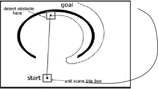
Figure 4.1 Situation of with and without path finding algorithm (Amit 2004)
SEARCH ALGORITHMS
The main purpose of search algorithms is to find the shortest path with the cheapest cost. The aim is to find the best path by using as little memory as possible in the shortest time. There are many common algorithms, and they can be ranged from the simplest to the most complicated. Overall, the search algorithms can be categorized into two parts; the brute-force search and the heuristic search.
Brute-Force Search / Blind Search
Brute-force search is the most popular search algorithm. It is the simplest way to get the best route. Generally, it will go towards the goal and turns to another direction whenever an obstacle is met. It will keep tracing around the edges of obstacles repeatedly. Therefore, it is called “blind search” (Mattews 1999).
This approach does not require any domain specific knowledge of the game world. What it needs is a state description, a set of legal operators, an initial state and a description of the goal state. This approach form the basis of the following approaches - breadth-first search, bidirectional search, depth-first search, depth-first iterative-deepening search and uniform cost search (Korf 1998).
Breadth-First Search
Breadth-first search is a tree-like algorithm. The tree is generated hierarchically in top down manner until a solution is found. (Mattews 1999). Besides, the searching time is proportional to the tree size. It consumes more memory as the number of nodes increases. As a result, it is detrimentally in practice, and will exhaust the memory available on typical computer. However, it is guaranteed to find a shortest path as long as the cost of each node is the same.
Bidirectional Search
Bidirectional search consists of two breadth-first searches. Both start simultaneously, one start from initial position and the other on from goal position. They keep on searching until they find the same node (Mattews 1999). The path form the initial state is then concatenated with the inverse of the path from the goal state to form the complete solution path. Hence, it can be said as an algorithm that requires an explicit goal state instead of simply testing the goal condition.
Bidirectional search still guarantees optimal solutions. But, at the same time, it has double space bound problems as breadth-first search do (Korf 1998).
Depth-First Search
The breadth-first works on a list of first-in first-out (FIFO) queue while depth-first search treats the list as a last-in first-out (LIFO) stack (Korf 1998). The advantage of this approach is the space requirement. It is proportional to the search depth, as oppose to the exponential for breadth-first search. However, it has a possibility to span to infinite tree once it traverses only to the left-most path.
Depth-First Iterative-Deepening Search
A combination of the features from breadth-first and depth-first search is called depth-depth-first iterative-deepening search (DFID) (Stickel and Tyson 1985; Korf 1985). The depth-first iterative-deepening search is similar to depth-depth-first search. The main difference is the cut-off point starts at the straight line distance to the goal. Once all nodes up to that point have been expanded, the cut-off point is incremented and the search will be repeated.
Starting from depth level one DFID performs a depth-first search to level by level until the goal solution is obtained. DFID is guaranteed to be along the shortest path since it never generates a node unless it has a child node. The iteration will be terminated when solution is found. Therefore, the space complexity is not too high.
Dijkstra’s Algorithm
Dijkstra’s algorithm looks at the unprocessed neighbors of the node closest to the start, and sets the update distances. The distance is calculated based on the cost instead of the number of nodes from start point to the goal.
This algorithm expands the node that is farthest from the start node, so it ends up ‘stumbling’ into the goal node just like the breadth-first search. It is guaranteed to find the shortest path (Mattews 1999).
The set V is the set of all vertices in the graph G. The set E is the set of ordered pairs which represent connected vertices in the graph - if (u, v) belongs to E then there is a connection from vertex u to vertex v
Assume that the function w: V x V -> [0, ] describes the cost w(x, y) of moving from vertex x to vertex
y (non-negative cost). The cost of a path between two vertices is the sum of costs of the edges in that path. The cost of an edge can be thought of as (a generalisation of) the distance between those two vertices. For a given pair of vertices s, t in V, the algorithm finds the path from s to t with lowest cost (i.e. the shortest path).
The algorithm works by constructing a subgraph S such that the distance of any vertex v' (in S) from s is known to be a minimum within G. Initially S is simply the single vertex s, and the distance of s from itself is zero. Edges are added to S at each stage by
(a) identifying all the edges ei = (vi1,vi2) in G-S such that vi1 is in S and vi2 is in G, and then
The procedure for adding an edge ej to S maintains the property that the distances of all the vertices within S from s are known to be minimum.
A few subroutines implemented with Dijkstra's algorithm (Dijkstra.E. W. 1959):
Initialize-Single-Source (G,s) 1for each vertex v in V[G] 2 do d[v] := infinite 3 previous[v] := 0 4 d[s] := 0
Relax(u,v,w)
1if d[v] > d[u] + w(u,v) 2 then d[v] := d[u] + w(u,v) 3 previous[v] := u
v = Extract-Min(Q) searches for the vertex v in the vertex set Q that has the least d[v] value. That vertex is removed from the set Q and then returned.
Another version of the algorithm is given by Jonsson and Markus (1997):
Dijkstra(G,w,s)
1 Initialize-Single-Source(G,s) 2 S := empty set
7 for each vertex v which is a neighbour of u
8 do Relax(u,v,w)
A related problem is the traveling salesman problem, which is the problem of finding the shortest path that goes through every vertex exactly once, and returns to the start. That problem is NP-hard, so it cannot be solved by Dijkstra's algorithm (Dijkstra.E. W. 1959), nor by any other known polynomial-time algorithm.
Uniform-Cost Search
Instead of expanding the nodes based on the depth from the root in tree, uniform-cost search extends nodes according to the cost of the node from root. At each loop, the node, which is going to be expanded, is the one who has the lowest cost. The nodes are stored in a priority queue. This algorithm is also known as Dijkstra’s single source shortest-path algorithm (Dijkstra.E.W. 1959). Unfortunately, it also suffers the same problem as breadth-first search, which is memory limitation.
Heuristic Search
solution; this is because some solution will take a very long period to be solved.
Best-First Search
Best-first search is a search algorithm which optimises breadth first search by ordering all current paths according to some heuristic. The heuristic attempts to predict how close the end of a path is to a solution (Stout and Bryan 1999). Paths which are judged to be closer to a solution are extended first. Efficient selection of the current best candidate for extension is typically implemented using a priority queue.
Best-first algorithms are often used for path finding in combinatorial search. If a good evaluation function is provided, best first search may drastically cut down the amount of search that we have to do to find a solution. We may not find the best solution, but if a solution exists you will eventually find it, and there is a good chance of finding it quickly. If the evaluation function is no good then the performances will be at par with simpler search techniques such as depth first or breadth first. And if the evaluation function is very expensive and takes longer period to calculate, the benefits of cutting down on the amount of search may be outweighed by the costs of assigning a score.
A* Algorithm
which minimizes the total length or cost of the solution path. It combines advantages of breadth first search and best first search, where the shortest path is found first and the next node to be explored is potentially closest to the solution.
A* algorithm employs a "heuristic estimate"(Korf 1998) which ranks each node by an estimate of the best route that goes through that node (Koenig et al. 2001). It visits the nodes in order of this heuristic estimate. The A* algorithm is therefore an example of best-first search. In the A* algorithm the score which is assigned to a node is a combination of the cost of the path so far and the estimated cost to solution. This is normally expressed as an evaluation function f, which involves the sum of the values returned by two functions g and h, g returning the cost of the path (from initial state) to the node in question, and h returning an estimate of the remaining cost to the goal state:
f(Node) = g(Node) + h(Node)
The A* algorithm then looks the same as the simple best first algorithm, but we use this slightly more complex evaluation function. The only drawback in A* algorithm is the high memory consumption.
The algorithm (Jones and Heyes 2001) :
AStarSearch
s.g = 0 // s is the start node s.h = GoalDistEstimate( s ) s.f = s.g + s.h
s.parent = null push s on Open
pop node n from Open // n has the lowest f
if n is a goal node construct path return success
for each successor n' of n newg = n.g + cost(n,n') if n' is in Open or Closed, and n'.g < = newg
skip
n'.parent = n n'.g = newg
n'.h = GoalDistEstimate( n' ) n'.f = n'.g + n'.h
if n' is in Closed
remove it from Closed if n' is not yet in Open push n' on Open push n onto Closed
return failure // if no path found
Iterative-Deepening A* (IDA*)
cost does not exceed the estimated threshold. Besides requiring less memory, it also finds an optimal solution. Other benefits include easier to implement algorithm compared to A* and most often IDA* runs faster than A*.
SMOOTHING THE A* PATH
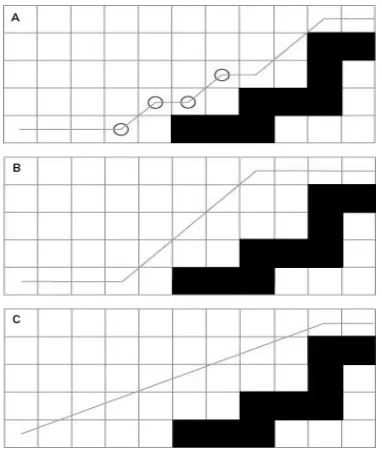
The first and most basic step in making an A* path more realistic is to remove the zigzag effect it produces, which you can see in Figure 4.2a. This effect is due to the fact that the standard A* algorithm searches the eight tiles surrounding a tile, and then proceeds to the next tile. This is acceptable in primitive games for smooth movement required in most games today.
Figure 4.2 The Common Zigzag Effect of the Standard (a) amodification with fewer, but still fairly dramatic turns, (b) and the most directed and hence desired route (c) (Stout 1999)
any neighboring blocked tile. Using the width of the unit, it checks the four points in a diamond pattern around the unit's center. The function returns true if it encounters no blocked tiles and false otherwise.
COMPARISON BETWEEN ALGORITHMS
Based on the literature, we found out that there are some differences between these algorithms. Obviously, brute-force search does not have the knowledge about the cost of the path to the goal in selecting the next node to span. On the contrary, the heuristic search plans the whole path before going anywhere. A comparison among the most popular search algorithms is listed in the Table 4.1 below
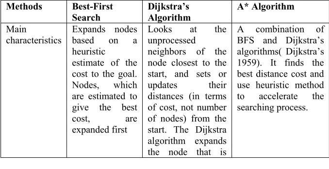
Table 4.1 Comparison between the algorithms
Methods Best-First Search Dijkstra’s Algorithm A* Algorithm Main characteristics Expands nodes based on a heuristic
estimate of the cost to the goal. Nodes, which are estimated to give the best cost, are expanded first
Looks at the unprocessed
neighbors of the node closest to the start, and sets or updates their distances (in terms of cost, not number of nodes) from the start. The Dijkstra algorithm expands the node that is
CONCLUSION
The comparison among the well-known path finding algorithms has been presented. It shows that A* provides the best solution with minimum cost. We believe A* which is widely used is the best path finding without doubt. A* algorithm is similar to Dijkstra's algorithm in which it can be used to find a shortest path. A* may not perform very well if the map is very large and the quality of the search depends on the quality of the estimated heuristic (Stout and Bryan 1999). The emergence of variations of A* algorithm together with genetic algorithm, neural networks and reinforcement learning are for a better and realistic path finding algorithms.
farthest from the start node, so it
ends up "stumbling" into the
goal node.
Reliability Guarantee to
find a shortest path.
Guarantee to find a best path.
Guarantee to find a best path as long as the heuristic estimate is admissible.
Processing time
Fast. Slow. Fast.
Heuristic estimation
Uses heuristic estimation.
Not using any heuristic estimation.
Uses heuristic estimation.
Memory consumption
REFERENCE
AMIT .2004. Citing Internet Sources URL http://theory.stanford.edu/~amitp/GameProgramming/ AStarComparison.html.
BJ”ORNSSON, Y., ENZENBERGER, M, HOLTE, R, SCHAEFFER, J. AND YAP, P. Comparison of Different Grid Abstraction for Pathfinding on Maps.
CORMEN, T. H., LEISERSON, C. E., RIVEST R. L. 1990.
Introduction to Algorithms. The MIT
Press/McGraw-Hill.
DIJKSTRA, E. W. 1959. A note on Two Problems in Connexion with Graphs. Numerische Mathematic. 1:269-271
DIABLO, SENIOR. 20 December 2003. Citing Internet sources URL http://ai-depot.com/Tutorial/PathFinding.html.
JÖNSSON, F. MARKUS. 1997. An Optimal Pathfinder for Vehicles in Real-World Digital Terrain Maps. Master Thesis, The Royal Institute of Science, School of Engineering Physics, Stockholm, Sweden.
JONES, JUSTIN HEYES. 2 September 2001. Citing Internet
sources URL http://www.geocities.com/jheyesjones/pseudocode.htm
l.
KOENIG, S.; LIKACHEV, M.; AND FURCY, D. 2001. Lifelong Planning A*. Technical Report, GIT-COGSCI-2002/2, College of Computing, Georgia Institute of Technology, Atlanta (Georgia).
KORF, R. E.1985. Depth-first iterative-deepening: An Optimal admissible Tree Search. Artificial
KORF, R. E. 1998. Artificial Intelligence Search Algorithms,
Algorithm and Theory of Computation Handbook.
Reading, Mass: CRC Press.
LESTER, PATRICK. 2 March 2003. Citing Internet sources URLhttp://www.policyalmanac.org/games/aStarTutori al.htm.
MATTEWS. 27 February 1999. Pathfinding: A Comparison between Algorithms.
STICKEL, M. E. AND TYSON, W. M. 1985. An Analysis of Consecutivelt bounded depth-first search with Applications in Automated Deduction. In Proceedings of the International Joing Conference on Artificial Intelligence (IJCAI-85), 1073-1075. Los Angeles, Ca. STOUT, BRYAN. 12 February 1999. Citing Internet sources
URLhttp://www.gamasutra.com/features/19990212/sm _01.htm.