Article
Mathematical modeling of rogue waves: A survey of
recent and emerging mathematical methods and
solutions.
Sergio Manzetti†,‡ ID*
1 Uppsala University, BMC, Dept Mol. Cell Biol, Box 596, SE-75124 Uppsala. Sweden; email:
2 Fjordforsk A/S, Midtun, 6894 Vangsnes. Norway; email: [email protected]
* Correspondence: [email protected]; Tel.: +47-4017-6707 † Current address: Fjordforsk A/S, Midtun, 6894 Vangsnes
1
2
3
4
5
6
7
8
9
10
11
12
13
14
15
16
Abstract: Anomalous waves and rogue events are closely associated with irregularities and unexpected events occurring at various levels of physics, such as in optics, in oceans and in the atmosphere. Mathematical modeling of rogue waves is a highly actual field of research, which has evolved over the last decades into a specialized part of mathematical physics. The applications of the mathematical models for rogue events is directly relevant to technology development for prediction of rogue ocean waves, and for signal processing in quantum units. In this survey, a comprehensive perspective of the most recent developments in methods for representing rogue waves is given, along with discussion of the devised and forms and solutions. The standard nonlinear Schrödinger equation, the Hirota equation, the MMT equation and further to other models are discussed, and their properties highlighted. This survey shows that the most recent advancement in modeling rogue waves give models which can be used to establish methods for prediction of rogue waves at open seas, which is important for the safety and activity of marine vessels and installations. The study further puts emphasis on the difference between the methods, and how the resulting models form a basis for representing rogue waves in various forms, solitary or with a wave-background. This review has also a pedagogic component directed towards students and interested non-experts, and forms a complete survey of the most conventional and emerging methods published until recently.
Keywords: rogue; wave; models; KdV; NLSE; non-local; ocean; optics 17
1. Introduction 18
Anomalous waves, or “rogue waves”, represent a rare phenomenon at sea which occurs on 19
multiple occasions yearly [1,2] and cause yearly millions of dollars of loss of cargo and loss of lives 20
[3]. Rogue waves are abnormally elevated waves, with a 2-3X height of the average wave normal and 21
with unusually steep shapes [4,5]. Rogue waves were recorded for the first time in 1995 during a 22
winter storm in the North Sea, when the “New Years Wave” hit the Draupner platform with a wave 23
height of 27 meters and 2.25X the average wave height [4]. The laser-installation on the deck, which 24
regularly records the elevation of the platform over the sea bed, registered the solitary giant wave 25
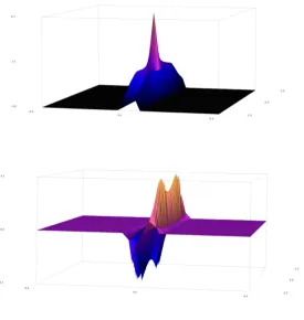
with its 15.4 m elevation above and 11,6 meter below the zero-level [4]. The shape of the wave was 26
symmetrical (Fig 1) with a Gaussian-bell shape and with a particular narrow wavelength. This shape 27
and behavior of anomalous waves is conserved across several observations made in the last 25 years, 28
including the rogue wave that hit the North Alwyn platform in November 1997 [6], the Gorm platform 29
in 1984 [6] and from Storm 172 on the North Alwyn field 100 miles east of Shetland [5]. The latter was 30
particularly unusual, with a height 3.19X the average (Fig 1). 31
. 32
33
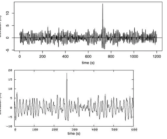
Figure 1. The laser-readings of the most extreme rogue wave registered (top), which hit the 34
the North Alwyn platform east of Shetland [5], reaching 18.04 meters and a ratio of 3.19X with 35
surrounding waves. Bottom: The New Years wave registered in 1995 on the Draupner platform (top) 36
in the North Sea. 37
38
Rogue waves are known to have sunk over 20 supercarriers since 1970 [6] and carry a force of 39
16-20 times (100 metric ton/m2) that of a 12 meter wave, and can easily break ship structures which 40
are designed to withstand far lower impact forces (6 metric ton/m2) [3]. Rogue waves are an eminent 41
threat to shipping and naval activities, and increase in prevalence with climate-change weather patterns 42
[7]. In this context, the insurance sector has searched for new models for predicting rogue waves and 43
for fortifying naval structures [3], as both off-shore installations, shipping and also cruise-ships have 44
been increasingly exposed to rogue waves in the last decades [3,6]. This development has also sparked 45
the project “Max Wave” [2] which has contributed with new models and algorithms for predicting 46
rogue waves by the use of satellite observation data. Rogue waves occur also in optical systems [8] in 47
the atmosphere [9], in plasma [10] as well as in molecular systems during chemical reactions [11]. 48
Earlier mathematical models and derived algorithms that were used to predict wave patterns were 49
originally developed by using the linear Gaussian random model, and rogue phenomena at sea 50
were largely disregarded as superstition. The linear Gaussian model is essentially a superposition 51
of elementary waves and predicts the occurrence of a rogue event at a very low probability. This 52
low probability is however incorrect accounting for the laser-readings made in the last 2 decades 53
at off-shore installations. Non-linear models which show a better agreement with the frequency 54
of rogue events at sea, are therefore gradually replacing the Gaussian model used in the insurance 55
industry. Non-linear models have been studied by several groups, and include the modified non-linear 56
Schrödinger Equation (NLSE) [6], the Peregrine soliton model [12] the Levi-Civita and Nekrasov 57
models [13,14], the Davey–Stewartson model [15], the fourth order partial differential equation 58
of Kadomtsev–Petviashvili, the one-dimensional Korteweg–de Vries equation for shallow water 59
surfaces, the second-order Zakharov partial differential equation [16], and the fully nonlinear potential 60
equations. Other systems have recently been developed, and are here reviewed in detail given their 61
equation [17], the Akhmediev model [18–21], and the recent models developed by Cousins and Sapsis 63
[22–24]. 64
2. The non-linear Schrödinger equation in prediction of rogue-waves 65
Rogue waves occur both in oceans as well as in optical systems [12], as well as in other 66
wave-systems (see above). For fiber optical systems, rogue waves are normally entirely 67
one-dimensional, however two-dimensional rogue waves have been recently documented, by 68
the form of the two-dimensional dissipative rogue waves [25]. These recently discovered optical 69
rogue waves occur when a delayed feedback is generated in the transverse plane of the the cavity, 70
forming an overlap of counter-directional fiber-optic signals, which leads to a rogue amplitude 71
[25]. These two-dimensional signals in optical systems are described by an own form of PDE, the 72
Lugiato-Lefever equation [26], which allows for 2D rogue wave solutions to be modelled without 73
collapse dynamics. This model is also used for describing a large spectrum of nonlinear phenomena in 74
optical systems, such as bistability, localized structures, self-pulsating localized structures and also 75
complex spatiotemporal behavior through an extended quasi-periodicity [27]. Rogue waves formed 76
in fiber optic systems have also been recently considered as a new field of research in optics, given 77
their anharmonic and nonlinear properties which can be a future application optical technologies 78
[28]. In particular, an own class of rogue waves which have the potential for application in optical 79
technologies are the self-similar pulses [29–32]. Self-similar pulses are wave-amplitudes measured in 80
fiber amplifiers [33], which experience an optical gain together with a Kerr-nonlinearity (Fig 2). 81
82
. 83
84
Figure 2. Observed Kerr-Nonlinearity in a crystal exposed to a magnetic field. [34]. Reprinted 85
with permissions.c Copyright OSA Publishing. 86
87
During the induction of the self-similar impulse in the solid, a fluid or any wave-carrying 88
medium, the shape of the resulting rogue wave no longer depends on the shape or duration of 89
the seed pulses, but depends only on the seed pulse energy (chirping). This creates a large effect 90
on the amplitude, which is largely independent on the initial conditions of the wave pattern. This 91
event, or formation of a rogue component in the wave-train, has also been observed in ocean wave 92
systems [35] and has attracted various groups to develop prediciton methods using the variations of 93
the non-linear Schrödinger equation (NLSE) [17,29,33,36,37]. One group in particular developed the 94
variable coefficient inhomogenous nonlinear Schrödinger equation (vci-NLSE) for optical signals [17]: 95
iψx+1
2β(x)ψtt+χ(x)|ψ|
2
ψ+α(x)t2ψ=iγ(x)ψ, (1)
which derives from the Zakharov equation [38]. Hereψ(t,x)is the complex function for the
96
function. The parameterα(x)defines the normalized loss rate and the functionα(x)t accounts for the
98
chirping effects (which indicates that the initial chirping parameter is the square of the normalized 99
growth rate). The parameterβ(x)defines the group-velocity dispersion (i.e. for an entire wave-train),
100
whileχ(x)defines non-linearity parameters, andγ(x)defines loss or gain effects of the wave-signal.
101
This equation is adaptable both for oceanic waves, as well as for optical non-linear wave guides. 102
Equation (1) is essentially the same as the generalized Gross-Pitaevskii equation with the harmonic 103
oscillator potentials in the Bose-Einstein condensates [39] and can be solved by applying the similarity 104
transformation [40] by replacingψ(t,x)in equation (1) with:
105
ψ(t,x) =ρ(x)Ψ(T,X)eiφ(t,x), (2)
whereρ(x) is the amplitude, and T and X represent the differential functions describing the
106
original propagation distance and the similarity variable, whileφ(t,x)is the linear variable function of
107
the exponential term, which all must be considered well to avoid singularity of the systemψ(t,x) [17].
108
T and X are given as: 109
T= t−tc(x)
W(x) (3)
X=
Z z
0
β(s)
W2(s)ds (4)
and hence the similarity transformation gives: 110
iΨX+1
2ΨTT+|Ψ|
2Ψ=0, (5)
which is the standard non-linear Schrödinger equation. 111
112
The transformation and integrability conditions derived by [17] show that the factors of the 113
wave system, such as effective wave propagation, distance, central position amplitude, the width 114
and phase of the pulse are ultimately dependent on the group velocity dispersion and on the 115
non-linearity parameters of the system (α,β,γ,χ). The “self-similar” solution found in the process
116
of the transformation of the variable coefficient inhomogenous nonlinear Schrödinger equation into 117
the standard nonlinear Schrödinger equation can ultimately be controlled under dispersion and 118
non-linearity management [17]. Once transformed from the iNLSE, the solutions to the NLSE are 119
derived by the derivation of polynomial conjugates to the root exponential function. This process is 120
reviewed in detail here from the studies by [19]. 121
2.1. The solutions to the NLSE 122
The NLSE equation has been solved by various groups, including [16,19,40–42]. Following one 123
of the most recent works by [18,19] in particular, the steps for deriving exact solutions to the NLSE 124
are defined by identifying rational solutions [18] for the homogenous nonlinear system in eqn. (5) 125
by using the Darboux transformation [43]. This method is often used to derive rational solutions for 126
non-linear systems and is adaptable to specific optical rogue waves as well as ocean rogue waves, 127
when represented by the NLSE. The main definition of a rogue event is that the wave “appears from 128
nowhere and vanish without a trace”, which is feature partly related to the behavior of solitons, which 129
are independent waves that self-propagate and exit a collision unchanged. The origin of solitons arises 130
from the first observation of a single solitary wave in the North Sea, made in 1834 by J. S. Russell, 131
who later reproduced the solitary wave in a tank. Since then, solitons have been mainly studied in 132
optical systems, and are represented as solutions to several types of nonlinear PDEs, including the 133
NLSE, the Korteweg de Vries equation and the Sine-Gordon equation. This type of rogue behavior, 134
system instability to the top of a plane wave amplitude, which is transferred to the highest amplitude 136
and then decays exponentially towards zero [18]. This behaviour is represented by Ma-solitons and 137
by Akhmediev breathers or “Akhmediev solitons” [18,19,44–46]. The difference between these two 138
soliton models lies in the initial conditions, where the Ma-solitons originates from the initial conditions 139
while the Akhmediev solitons arise during evolution of the system given by modulation instability 140
[44,47,48]. 141
When solving the NLSE according to the Akhmediev scheme [19] , their method describes the 142
modeled envelope function (ψ) as a solution ranked into an order of hierarchy, starting from first,
143
and progressing to the second, third or fourth order [19]. The difference between each order is the 144
increasing amplitude of the rogue wave (first order -lowest amplitude, fourth order sharpest peak 145
and highest amplitude). The envelope functionψis expressed as a ratio of polynomials multiplied
146
to the complex exponential root function,eix. The polynomials, which are given by functions of 147
variable x and t, are identified by performing the Darboux transformation on the NLSE system [19]. 148
Akhmediev and colleagues furthermore apply a compatibility-check between the root functioneixand
149
the reference-state for two specified column matrix elements, which define initial conditions for the 150
NLSE. These matrix elements (vectors) are given specifically by Akhmediev and colleagues [19] as 151
two differential equations: 152
rx=il2r+ilψ∗s−il2|ψ|2r+1
2ψ
∗
s (6)
sx=il2s+ilψr−1
2ψtr+ i
2|ψ|2s (7)
which are split into real and imaginary parts, before being simplified and solved to fit into the 153
modified Darboux scheme [19,43] to give the two linear differential forms: 154
rl(x,t) =
√ 2
xt−1 2+ix
e−ix/2 (8)
sl(x,t) =
√ 2
x−i(t+1
2)
e−ix/2 (9)
Where the two vectors (8), (9) are used in the Darboux scheme to findψj, wherejis the order of
155
hierarchy. The general solution to the NLSE, derived from this scheme [19] is given by the following 156
general form (for any order in the hierarchy): 157
ψj(x,t) =
(−1)j+ Gj(x,t) +ixHj(x,t)
Dj(x,t)
eix (10)
where G, H and D are the polynomials of the two variables x and t (mentioned above). The first 158
order-solution [19] has the following polynomials: G = 1, H = 2 andD=1+4t2+4x2which give the 159
following envelope function (shown in Fig 3): 160
ψl =
1−4 1+2ix 1+4t2+4x2
. 161
162
Figure 3. The plot ofψ1, the first-order solution to the standard NLSE [19]. Real and imaginary
163
part shown respectively above and below. Plotted with SageMATH [49,50]. 164
165
For the second-order solution, [19] identify the vectors r2 and s2 by solving the equations (6) and 166
(7) by using the form ofψgiven in (10). This gives the second-order solution:
167
ψ2(x,t) =
(−1)2+
−2t4−12t2x2+ix8t2x2+2t2−4x4−2x2+154−3t2−10x4−9x2+38
16t6
3 +13t2+ 16x6
3 +36x4+33x2+34
eix (12) which is shown in figure 4. The third and fourth order rational solutions are furthermore 168
. 170
171
Figure 4. The plot of ψ2, the second-order solution to the standard NLSE [19]. Real and
172
imaginary part shown respectively above and below. Plotted with SageMATH [49,50]. 173
174
The same hierarchy-dependency is given in the approach by [17], for the transformed vci-NLSE, 175
who define the general solutions for the NLSE in the hierarchicaln-th order given by: 176
ψn= 1
W
s β
χ[(−1)
−1+Gn+i(Z−Z0)Hn
Fn
×ei[(1−v
2
2)(Z−Z0)+vT+φ] (13)
where each factor is given for the first and second order rational solutions [17]. Similarly to the 177
hierarchy solutions of Akhmediev [19], the increasing order gives higher and higher rogue waves, 178
compared to their surrounding waves. The first and second order rational solutions given in [17] 179
reflect respectively a 3X and 5X rogue wave height, compared to the surrounding waves. For plots of 180
these, refer to [17]. 181
182
The similarity between (13) and (10) is striking, and both retain the basic form of a complex 183
polynomial multiplied by a complex exponential root function giving soliton solutions. The root 184
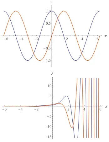
functions of (10) and (13) are shown in their generic form in Fig 5, which depicts the distinction 185
between the seed pulse for the regular NLSE and the vci-NLSE, as studied respectively by [17,19] for 186
. 188
189
Figure 5. The root functions for the standard NLSE and the inhomogenous variable coefficient 190
NLSE. Top: The seed impulse used in the solutions to the standard NLSEm,eix [19]. A generic 191
form of the seed impulse used in the solutions of the inhomogenous variable coefficient NLSE [17] 192
(f(x) =ei(1−x2/2)+x. Real part (Blue) and imaginary part (Red).
193
194
The root function for the vci-NLSE (Fig 5) shows its specific pattern of wave accumulation, which is 195
similar to the formation of wave packets. This pattern is conserved with the physical behavior of rogue 196
wave formation, where the rogue wave forms during a focusing phase [51]. Other approaches used to 197
solve the NLSE have been given by [37], who used the inverse scattering method of transformation, 198
which is a generalization of the Fourier analysis. Their solutions differ from the methods discussed 199
above, and are periodic and ascribed by a complex envelope function for the deep water train with 200
added higher-order terms from the perturbation procedure [37] One of the solutions are shown in 201
figure 6, which shows the following variant of the Osborne models: 202
ψ= cos(
√
2x)sech(√2t) +i√2tanh(2t)
√
2−cos(√2x)sech(√2t) e
which is a periodic function in space, derived from the general form given in [37], shown in 203
Figure 6. 204
. 205
206
Figure 6. The selected wavefunction from the Osborne models [37]. Top: Real part; Bottom: 207
Imaginary part. Plotted with SAGEMATH [49,50] 208
209
The disadvantage of this system, compared to single-peak models derived from [19] lies in their 210
periodicity and multiple peaks, while the rational solutions behind the single peak models of [18,19] 211
are the first in general to serve as prototypes for rogue waves. 212
3. The Korteweg de Vries equation 213
Wave systems defined by higher order nonlinear PDEs, such as (2), can be solved also by the 214
bilinearization technique [52]. This technique involves the step of transforming the differential 215
equation into a more tractable form by replacing the unknown time- and position-dependent envelope 216
function with a new form [52]. After this replacement has been performed, the bilinearization 217
technique applies Hirota bilinear operators for a modified Bäcklund transformation technique [53], 218
which assists in rewriting the original PDE into a simplified PDE composed of bilinear operators, from 219
where exact soliton solutions can be identified. The most suitable example [52] for the application of 220
the bilinearization technique is on the Korteweg de Vries (KdV) equation: 221
Ψt+6ΨΨx+Ψxxx =0 (15)
where the boundary conditions are thatψ→0 as|x| →∞. The real wavefunction is differentiated
222
according to the spatial and temporal dimensions as denoted. In the bilinearization technique, a 223
transformation of the wavefunction to another form is the first step, where an ideal steady-state form 224
is proposed [52] to: 225
ψ(x,t) = (p2/2)sech2(η/2), (16)
η=px−p3t+η0, (17)
andη0and p are arbitrary constants. By the bilinearization technique [52], one can rewrite (16) to
227
the form: 228
ψ(x,t) =2p2(eη/2+e−η/2), (18)
which is converted to its functional form: 229
ψ(x,t) =2∂
2ln[f(x,t)]
∂x2 , (19)
with f(x) = 1+eη. 230
The bilinearization technique [52] substitutes (19) into the original KdV equation (15) and 231
integrates it with respect to x: 232
fxtf− fxft+ fxxxxf −4fxxxfx+3(fxx)2=0 (20)
which is the original version of the bilinearized variant of the Korteweg de Vries equation (15) as 233
derived by [53]. The solution to (20), f(x) = 1+eη, is defined as a more fundamental quantity thanψin 234
eqn. (18) for the structure of the original nonlinear PDE in eqn. (15). In the method of bilinearization, 235
the Hirota bilinear operators are introduced. These are defined by the following definition [53]: 236
DntDmxa·b= (∂/∂t−∂/∂t0)n(∂/∂t−∂/∂t0)ma(x,t)b(x0,t0)|x=x0,t0=t (21)
withmandnbeing arbitrary positive integers. At this stage, the converted form of the KdV 237
equation (20) is rewritten as a PDE composed of Hirota operators: 238
Dx(Dt+D3x)f· f =0, (22)
which is a simplified form for the identification of exact solutions using the Bäcklund 239
transformation for the original nonlinear PDE (15). The exact solution structure for the type of 240
Hirota-operator based PDE form (22) of the KdV equation (15) is given by: 241
Ψ=1+e(eη1+eη2)−e2F(Ω1−Ω2,p1−p2)
F(Ω1+Ω2,p1+p2)
eη1+η2 (23)
which represents the two-solition solution to the original KdV equation (15). η1 and η2are
242
the functions with the independent variables x and t as given in (16) for each of the solitons, and 243
Ω1 = −p31andΩ2 = −p32, following the same definition for (16) for each soliton. ηrepresent the
244
perturbations [52]. The KdV equation (15) has also been solved by Matveev by identifying positon 245
solutions [54], which exert the same behavior as solitons, such as conserved shape after collision, and 246
elastic collision behavior. The positon differs from the soliton in that it has an infinite energy, and is 247
therefore not a strong model for oceanic or optical rogue waves. Positons have however a tendency 248
to represent smoother solutions than solitons to the KdV equation, and can have very high peaks 249
compared to the wave normal. The KdW equation has also been solved by a nonlinear Fourier method 250
[55,56], which is represented by a superposition of nonlinear oscillatory modes of the wave-spectrum. 251
This model, developed by Osborne [55,56], has a capacity to include a large number of non-linear 252
oscillatory patterns, also known as multi-quasi-cnoidal waves, which are used to form the rogue wave 253
by superposition in constructive phases. These solutions to the original KdV equation (15) include 254
several solitons, depending on the number of degrees of freedom selected for the numerical simulation 255
of the KdV equation. This yields a 3D wave complex composed of solitons and radiation components 256
4. The extended Dysthe equation 258
In 1979, Dysthe [57] developed a modification of the perturbation-based NLSE by adding an 259
additional term to the third-order perturbation variant originally developed by Higgins [58]. Dysthe’s 260
method gave an NLSE variant, known as the extended Dysthe equation, which showed to have a 261
better agreement with the mean flow response to non-uniformities in deep-water waves. The extended 262
Dysthe equation is given by: 263
i
kψxyy+ψyy+2ikψx+2ψz=oe
4, (24)
where the inhomogenous component is the fourth-order perturbation defined by Dysthe [57]. 264
Dysthe transformed this equation to standard NLSE using dimensionless variables, and added the 265
following perturbation to the general solution: 266
ψ=c0(1+α)ei(θ 0−1
2ic20t) (25)
whereαandθare small real perturbations of the amplitude and phase respectively. After insertion
267
of (25) in the dimensionless form of (24) and linearizing, Dysthe obtained a simplified system of two 268
PDEs, where the respective plane-wave solutions are in the form: 269
α0
θ0 !
∝ei(λx+µy−Ωt) (26)
and 270
φ∝e[Kz+i(λx+µy−Ωt)] (27)
where K =p(λ2+µ2)andλ,µandΩare selected parameters which satisfy a set of dispersion
271
relations given by Dysthe [57]. 272
The stability of the solutions derived by Dysthe shows that the Dysthe equation represents a 273
more realistic model than the NLSE, given that it does not predicts a maximum growth rate for all 274
wavevectors, but only for some wavevectors only. This displays that the fourth-order perturbation 275
term added to the NLSE gives a considerable improvement to the results relating to the stability of 276
the finite amplitude wave. It is particularly the first derivative by the transformed variables in the x 277
and z dimensions in eqn. (24) which contributes to the excellent results of Dysthe. Dysthe and Trulsen 278
[59,60] further developed this equation by including up to the fifth-order of the derivative of the wave 279
amplitude describing the linear dispersive terms, and simulated successfully [61] the New Year’s 280
wave [4] using the extended Dysthe equation [57,61]. 281
5. The MMT model 282
The MMT equation is a one-dimensional nonlinear dispersion equation which was originally 283
proposed by Majda, McLaughlin and Tabak [62]. The MMT equation gives soliton-like solutions 284
which have been analyzed in detail by Zhakarov [63–65] and gives four-wave resonant interaction 285
between waves, which, when coupled with large scale forces and small-scale damping, yields a family 286
of solutions which exhibit direct and inverse cascades [22]. The MMT equation is given by: 287
iψt=|∂x|α+λ|∂x|β/4(||∂x|β/4ψ|2|∂x|β/4ψ) +iDψ (28)
whereψis a complex scalar and|∂x|αis the pseudodifferential operator defined on the real axis
288
through the Fourier transform: 289
The last term in (28) is the dissipation term, which is tuned to fit ocean waves through the 290
Laplacian operator, Dψ, defined in the Fourier space:
291
d
Dψ(k) = (
−(|k| −k∗)2 b
ψ(k) |k|>k∗
0 |k|6k∗ (30)
This dissipation term, used by [22] is similar to other dissipation models used by Komen and 292
colleagues [66], who have developed concrete models for simulating large wave groups with focusing 293
and defocusing effects.λis the nonlinearity coefficient and corresponds to the focusing phase when
294
<0, and to the defocusing phase when>0. The MMT equation (28) differs from the standard NLSE 295
by that its family of solutions develop in a more exponential pattern, rather then the Gaussian-bell 296
shaped pattern observed for the solutions for the NLSE [22]. The interesting aspect of this pattern 297
of the spectrum of solutions of the MMT equation is in the mode of formation of the rogue wave, 298
where there energy is transferred from and to the surrounding waves. The solutions are in other words 299
induced by the intermittent formation from the localized rogue event arising out from the regular 300
Gaussian background and collapsing into the surrounding waves. The energy of the rogue wave is 301
transferred to the surroundings and experiences a complete zero-point state, merging completely in 302
the background [22]. 303
The MMT model shows also the formation of quasisolitons which appear in triple-wave packets, 304
as modelled by Zakharov and Pushkarev [63] and differ from regular solitons in that they radiate 305
the energy backwards towards the preceding amplitudes. This behavior of the solutions may be 306
particularly compatible with the simulation of rogue wave events occurring in regions with strong 307
counter-wind currents, such as in the Aghulas-current [67] or in the regions of the Irish sea [2], which 308
are heavily populated by rogue events, on the passage of the warm waters of the Gulf stream when 309
encountering the frequent low-pressure systems over the Irish sea with counter-wave winds. The 310
quasibreathers or quasisolitons [63], have the root function similar to the Dysthe-type solutions given 311
in (25). Zakharov and Pushkarev [63] approach the solutions in the form: 312
ψ(t) =ei(Ω−kV)tφk (31)
whereΩ and V are constants (Ω < 0 and V > 0 ), and k is the wavenumber, which is an 313
approximate solution to the soliton-like solution for the MMT model. In this approximation, [63] give 314
φk the following form:
315
φk=λ R
T1234φ∗1φ2φ3δ(k+k1−k2−k3)dk1dk2dk3
−Ω+kV− |k|α , (32) which represent a form which gives quasi-soliton solutions [68] to the MMT equation. This form 316
of the solutions to the MMT equation radiates energy backwards to the proceeding amplitudes, and 317
represents therefore an energy-focusing which is rather un-similar from the focusing effects modeled 318
by others for rogue patterns (vide supra). It is interesting to note that backward radiation plays also 319
a central role for the dynamics of the quasi-solitons, and not only for their energy-accumulation 320
profile. Using the MMT model, Zakharov and Pushkarev [63] developed also a model for collapses of 321
the rogue event, by using self-similar solutions, and model the formation of the wave wedge in the 322
appearing and vanishing state, given by a Fourier-space distribution of the wave-function. Zakharov 323
and Pushkarev [63] have also used the MMT model to develop turbulence-based solution for the 324
localized rogue event, using the initial condition in the form of a NLSE soliton: 325
ψ(x, 0) = q
2k9/4m
eikmx
cosh(qx), (33)
which shows a conserved action and momentum, and an “inner turbulence” localized both in the 326
is described by the authors in affecting the form of its wave-spectra, which is irregular and with a 328
stochastic behavior [63]. This model of the rogue wave shows quasi-periodic oscillations with slowly 329
diminishing amplitudes over time – caused by the destruction of rogue wave by the surrounding 330
interference, which the authors denoted as a "quasi-breather". 331
6. The Hirota equation 332
Multisolitons and breathers for rogue waves have been also successfully modeled [69] by applying 333
the Darboux transformation on the Hirota equation [53]. In their approach, Tao and He [69] developed 334
the Lax pair on the Hirota equation, by using the AKNS [70] procedure to get the Lax pair with the 335
spectral parameters of the Hirota equation given below: 336
iψt+α(2|ψ|2ψ+ψxx) +iβ(ψxxx+6|ψ|2ψx=0 (34)
where the Lax pair is expressed as 337
φx=Mφ,φt=Nφ (35)
gives rise to the extended matrix representation of the operators in the Hirota equation as 338
described by Tao and He [69]. Tao and He further applied the Darboux transformation [43] on the 339
Lax-represented system by using the simple gauge transformation for spectral problems, 340
φ[1]=Tφ (36)
where T is the polynomial applied on the parameterλgiven in the Lax pair, andφis the seed
341
function. Tao and He [69] argue however that regular seed solutionφ = eix as described in the
342
previous sections is too special, and makes the rogue wave model not universal enough. Tao and 343
He develop therefore a different seed function compared to Akhmediev and colleagues [19,44] for 344
instance, and develop a more extended form of the seed function by starting from a zero seed solution 345
and a periodic seed solution to construct the complete solutions for the breathers and solitons. At zero 346
seed and with the parameterλfrom the Lax pair they set the following Hermitian seed pair:
347
φ=e−i(ξ+iη)x−(4βi(ξ+iη)
3+2αi(ξ+iη)2t
(37)
and 348
φ∗=ei(ξ+iη)x+(4βi(ξ+iη)
3+2αi(ξ+iη)2t
(38)
back in the Darboux Transformation to get the 1-soliton solution: 349
ψ[1]soliton=2ηe2i(−iξx−4βξ3t−2αξ2t+12βξη2t+2αη2t)×sech(−2ηx−24βη2t+8βη3t−8αηξt). (39)
Tao and He [69] further report the model for the 2-soliton solution, and finally give the form of 350
the 1-soliton breather solution: 351
ψbreather[1] =eiφ "
c−2η[ηcosh(2d2)−iσsinh(2d2)−ccos(2d1] ccosh(2d2)−ηcos(2d1)
, (40)
whered1,d2,σare given [69]. Tao and He finally construct the Rogue wave solutions to the
352
original Hirota equation in (34) by Taylor expansion on the breather solutions in (40). The Taylor 353
expansion is carried out at theηvariable of the breather solution (40) which is given in [69], and forms
354
ψroguewave=kei(−2ξx+βt)
1−2k1+2k2+ik3t k1−k2
(41)
where the polynomialsk1,k2,k3are given by Tao and He [69]. The rogue wave model resulting
356
from this form is more general than the model given by Akhmediev and collegues [71] on the Hirota 357
equation. This difference is caused by the appearance of several parameters related to the eigenvalues 358
of the Lax pairs, and gives however a possibility to tune more finely the model to experiments on rogue 359
waves. This advantage of the model by Tao and He increases the ability to modulate the precision of 360
reproducing a rogue wave model by calculations. Tao and He’s method grants also the possibility in 361
calculating higher order rogue wave solutions to the Hirota equation by determinant representation of 362
the Darboux Transform, which was carried out in a subsequent work [72]. 363
7. The Ablowitz-Musslimani models: Non-local rogue waves 364
Another critical method for modelling rogue waves was developed by Ablowitz and Musslimani 365
[73–76] and uses nonlocal integrable models of the NLSE (1) and KdV (15) equations, where the 366
resulting wave is derived by reverse space-time symmetry. The model evolves by establishing 367
integrability by an infinite number of constants of motion or an infinite number of conservation 368
laws. By this, the method uses a compatible pair of linear equations (similar to the Lax pair in 369
the Hirota equation in (35)) with the nonlinear integrable equation. The method by Ablowitz and 370
Musslimani differs from the Hirota method in that the pair of linear equations represent the scattering 371
problem and the evolution of the scattering data [73,76]. Furthermore, the method by Ablowitz and 372
Musslimani is different from others in that it constructs an inverse scattering problem also known as a 373
linear Riemann-Hilbert problem, which gives the solution to the nonlinear PDE with dependency on 374
time. 375
The approach by Ablowitz and Musslimani [73] starts by linearizing the equation: 376
iqt(x,t) =qxx(x,t)±2q(x,t)q∗(−x,t)q(x,t), (42)
where one can immediately observe the existence of a Hermitian pair with reverse directional 377
variables. This form, where reverse variables are used, defines the nonlocal property of the equation 378
and has the advantage by that the equation remains invariant in time and space, after the complex 379
conjugate is taken. Hence, the nonlocal equation is parity- and time- symmetric (P T-symmetric), 380
which prevents the equation from yielding different results by a self-induced potential. 381
An exemplary Lax pair is given in [77] as: 382
vx= −ik q(x,t)
r(x,t) ik
!
v, (43)
vt= A B
C −A
!
v, (44)
wherevis the two-component vector andkis a special parameter, and A and B are complex 383
functions. Ablowitz and Musslimani use at this step specific compatibility conditions [78] to transform 384
the original PDE in (42) (i.e.ψxt=ψtx) and gains the simplified PDE pair:
385
iqt(x,t) =qxx(x,t)−2r(x,t)q2(x,t), (45)
−irt(x,t) =rxx(x,t)−2q(x,t)r2(x,t). (46)
which yield the original form in eqn. (42). Ablowitz and Musslimani further define the nonlocality 386
r(x,t) =∓q∗(−x,t). (47) This step is particularly characteristic to Ablowitz-Musslimani models [73–76], which of the new 388
class of nonlocal integrable evolution equations with the nonlocal NLSE hierarchy are directly derived 389
by. 390
The aforementioned property of conserved quantities and conservation laws is also characteristic to 391
Ablowitz-Musslimani models [73,75]. Here they define a set of eigenfunctions which obey specific 392
boundary conditions [73]. The eigenfunctions are very similar to the seed functions used by other 393
groups and when inserted in the Lax pair, yield a Riccati model of the conservation quantities. This 394
yields the global conservation laws which are given in [73] by: 395
C0= Z +∞
−∞ q(x,t)q
∗(−x,t)dx,
C1= Z +∞
−∞ [qx(x,t)q
∗
(−x,t) +q(x,t)q∗x(−x,t)]dx,
C2= Z +∞
−∞ [qx(x,t)q
∗
x(−x,t) +σq2(x,t)q∗2(−x,t)]dx,
which are real integrable Hamiltonians. Ablowitz and Musslimani [73] derive furthermore local 396
conservation laws defined by the equations: 397
∂t[q(x,t)q∗(−x,t)] +i∂x[q(x,t)q∗x(−x,t) +q∗(−x,t)qx(x,t)] =0 (48)
∂t[q(x,t)q∗x(−x,t)] +i∂x[q∗x(−x,t)qx(x,t) +q(x,t)q∗xx(−x,t)−σq2(x,t)q∗2(−x,t)] =0 (49)
which are used to develop the framework for the direct scattering problem and the inverse 398
scattering problem, where the scattering data is given by specific scattering matrices. The same 399
symmetry is also in the problem of the potential and in the eigenfunction and leads naturally to the 400
same symmetry relation in the scattering matrices, which are given by: 401
N(x,k) =ΛM∗(−x,−k∗) (50)
and 402
¯
N(x,k) =Λ−1M∗¯ (−x,−k∗), (51) where Λ is a 2x2 matrix with zeros in the diagonal and 1, ±1 on the lower and upper 403
diagonal respectively. For the inverse scattering problem, Ablowitz and Musslimani [73] account 404
for the symmetry condition by considering the set of basis terms as a left scattering problem, and 405
supplement these terms with the equivalent right-scattering problem, which from they formulate the 406
Riemann-Hilbert problem and find the linear integral equations which govern the functions M and ¯M 407
in (50). These equations are given by: 408
M(x,k) =
1 0
+
¯ J
∑
l=1¯
Ble2ik¯lxM¯(x, ¯kl)
k−k¯l
− 1 2πi
Z ∞
−∞
¯
R(ξ)e2iξxM¯(x,ζ)
ζ−(k+i0) dζ, (52)
¯
M(x,k) =
0 1
+
J
∑
l=1Ble2iklxM(x,kl)
k−kl
− 1 2πi
Z ∞
−∞
R(ξ)e2iξxM(x,ζ)
whereR(k)and ¯R(x)are the reflection coefficients. The termsBland ¯Blare the conservation law
409
Hamiltonians applied symmetrically. From this stage, Ablowitz and Musslimani [73] derive a linear 410
algebraic integral system of equations that solve the inverse problem for the eigenfunctions ¯M(x,k)
411
andM(x,k). 412
The resulting soliton solutions of the Ablowitz-Musslimani model assume hence the form 413
q(x) =− 2(η+η¯)e
iθ¯1e−4iη¯12te−2 ¯η1x
1+ei(θ1+θ¯1)e4i(η12−η¯21)te−2(η1+η¯1)x
, (54)
which represents a family of solutions defined by the four independent parameters which have a 414
dynamic relationship with the time-variable and which gradually develop a singularity in a finite time 415
period,tsat x=0 wheretsis given by:
416
ts =
(2n+1)π−θ1−θ¯1
4(η12−η¯12) . (55)
(55) is a critical form of the time-variable which distinguishes the method of Ablowitz-Musslimani 417
[73–78] from other rogue waves models and adds a non-linear evolution of the rogue wave. Ablowitz 418
and Musslimani have also most recently developed a new model which includes nonlocal rogue waves 419
with nonzero background, which provide and more realistic view of the rogue wave, which focuses 420
energy from neighboring waves [79]. 421
Solutions to the Ablowitz-Musslimani model (42) were also developed by Yang and Yang [80], who 422
used the Darboux transformation method on the PDE coupled with the Bäcklund transformation on 423
the potential functions, identifying three types of rogue waves from the Ablowitz-Musslimani picture. 424
Yang and Yang expanded the solutions to polynomials using Schur polynomials [80]. This analysis of 425
the Ablowitz-Musslimani model showed greater variation in the rogue waves compared to the regular 426
NLSE, where the variations were represented by the terms in the denominator of the soliton solutions. 427
The parity-time symmetry potential of the Ablowitz-Musslimani equations has also been studied by Yu 428
[81] very recently, who obtained discrete rogue wave solutions with three free parameters (refer to eqn. 429
(54) for similarities). Yu studies in particular the effect that the dispersion of the parity-time symmetry 430
has on the solutions, as well as the effect of the coefficients and the parameters. Yu [81] uses the 431
Darboux transformation method in a similar fashion to Yang and Yang [80] to derive different forms of 432
solitons with different height which are defined by two of the three free parameters in the solution (η
433
and ¯ηin eqn. (54)). Yu [81] also assesses the stability of rogue waves over a specific period of time, and
434
includes a modulation instability coefficient which allows the modelling of several discrete solutions 435
which represent various stages of a rogue wave formation (appearing suddenly and disappearing 436
suddenly), a property of rogue waves also reported by Akhmediev and colleagues [18–20]. Finally, Yu 437
models rogue waves which appear rapidly and do not disappear. This latter model may be particularly 438
relevant to describe rogue events during low-pressure systems at open sea, which have been reported 439
in several cases to give stable rogue waves with long life-time (i.e. the rogue waves reported in the 440
study by Munk [35]). 441
8. Conclusions 442
A survey of various mathematical models for representing rogue waves has here been carried out 443
to the maximum extent of including the most applied as well as most recent models. The overall survey 444
yields a perspective which delineates the common traits between the methods. This survey also shows 445
how novel and emerging models allow for better modelling of rogue waves, by including several 446
parameters associated with the evolution of the rogue waves, such as the duration, the height and 447
other particular properties that a rogue event can display when occurring in oceans, optical systems, 448
or even in the atmosphere. The results show also new the versatile forms of the older models (MMT 449
and Dysthe), can be furthermore adapted and studied numerically in upcoming papers, particularly 450
coast and on the Western Norwegian coast during North-East and North winds respectively. By the 452
overall review of the various methods, a theorem is suggested for describing the origin of rogue waves 453
in the ocean. The theorem suggests that a rogue wave in the ocean can be formed whenever there is a 454
momentaneous surplus of energy perturbed on the momentum or in the kinetic term of a wave-train, 455
induced either by a sudden change in the atmosphere leading to strong winds appearing suddenly 456
over large volumes of water, or induced by a collision of large volumes of water with highly different 457
temperatures and densities, or finally, as often observed, a rogue event occurs by the constructive 458
overlap of waves, in opposite directions, in transverse directions or running in the same direction 459
and its duration is determined, when occurring in the same direction, by the slight deviations in the 460
momenta of the overlapping waves. Future work will be the submission of a project proposal for 461
predicting rogue waves for off-shore structures, currently under development for the Norwegian 462
Research Council. 463
Funding:This research received no funding. 464
Conflicts of Interest:The author declares no conflict of interest. 465
Abbreviations 466
The following abbreviations are used in this manuscript: 467
468
MMT Majda, McLaughlin and Tabak AKNS Ablowitz, Kaup, Newell Segur 469
References. 470
471
1. Lehner, S.; Schulz-Stellenfleth, J.; Niedermeier, A.; Horstmann, J.; Rosenthal, W. Extreme waves detected by 472
satellite borne synthetic aperture radar. ASME 2002 21st International Conference on Offshore Mechanics 473
and Arctic Engineering. American Society of Mechanical Engineers, 2002, pp. 251–256. 474
2. Rosenthal, W.; Lehner, S. Rogue waves: Results of the MaxWave project. Journal of Offshore Mechanics and
475
Arctic Engineering2008,130, 021006. 476
3. Didenkulova, I.; Slunyaev, A.; Pelinovsky, E.; Kharif, C. Freak waves in 2005. Natural Hazards and Earth
477
System Science2006,6, 1007–1015. 478
4. Haver, S. A possible freak wave event measured at the Draupner Jacket January 1 1995. Rogue waves 2004
479
2004, pp. 1–8. 480
5. Stansell, P. Distributions of freak wave heights measured in the North Sea. Applied Ocean Research2004, 481
26, 35–48. 482
6. Dysthe, K.; Krogstad, H.E.; Müller, P. Oceanic rogue waves. Annu. Rev. Fluid Mech.2008,40, 287–310. 483
7. Weisse, R.Marine climate and climate change: storms, wind waves and storm surges; Springer Science & Business 484
Media, 2010. 485
8. Solli, D.; Ropers, C.; Koonath, P.; Jalali, B. Optical rogue waves.Nature2007,450, 1054. 486
9. Stenflo, L.; Marklund, M. Rogue waves in the atmosphere. Journal of Plasma Physics2010,76, 293–295. 487
10. Moslem, W.; Shukla, P.; Eliasson, B. Surface plasma rogue waves. EPL (Europhysics Letters)2011,96, 25002. 488
11. Tlidi, M.; Gandica, Y.; Sonnino, G.; Averlant, E.; Panajotov, K. Self-Replicating spots in the brusselator 489
model and extreme events in the one-dimensional case with delay. Entropy2016,18, 64. 490
12. Kibler, B.; Fatome, J.; Finot, C.; Millot, G.; Dias, F.; Genty, G.; Akhmediev, N.; Dudley, J.M. The Peregrine 491
soliton in nonlinear fibre optics.Nature Physics2010,6, 790. 492
13. Levi-Civita, T. Determination rigoureuse des ondes permanentes d’ampleur finie. Mathematische Annalen
493
1925,93, 264–314. 494
14. Nekrasov, A. On waves of permanent type.Izv. Ivanovo-Voznesensk. Politekhn. Inst1921,3, 52–65. 495
15. Smith, R. Giant waves. Journal of Fluid Mechanics1976,77, 417–431. 496
16. Zakharov, V.E. Collapse of Langmuir waves.Sov. Phys. JETP1972,35, 908–914. 497
17. Dai, C.Q.; Wang, Y.Y.; Tian, Q.; Zhang, J.F. The management and containment of self-similar rogue waves 498
18. Akhmediev, N.; Soto-Crespo, J.M.; Ankiewicz, A. Extreme waves that appear from nowhere: on the nature 500
of rogue waves. Physics Letters A2009,373, 2137–2145. 501
19. Akhmediev, N.; Ankiewicz, A.; Soto-Crespo, J. Rogue waves and rational solutions of the nonlinear 502
Schrödinger equation.Physical Review E2009,80, 026601. 503
20. Akhmediev, N.; Ankiewicz, A.; Soto-Crespo, J.; Dudley, J.M. Rogue wave early warning through spectral 504
measurements?Physics Letters A2011,375, 541–544. 505
21. Chabchoub, A.; Hoffmann, N.; Branger, H.; Kharif, C.; Akhmediev, N. Experiments on wind-perturbed 506
rogue wave hydrodynamics using the Peregrine breather model. Physics of Fluids2013,25, 101704. 507
22. Cousins, W.; Sapsis, T.P. Quantification and prediction of extreme events in a one-dimensional nonlinear 508
dispersive wave model. Physica D: Nonlinear Phenomena2014,280, 48–58. 509
23. Cousins, W.; Sapsis, T.P. Unsteady evolution of localized unidirectional deep-water wave groups. Physical
510
Review E2015,91, 063204. 511
24. Cousins, W.; Sapsis, T.P. Reduced-order precursors of rare events in unidirectional nonlinear water waves. 512
Journal of Fluid Mechanics2016,790, 368–388. 513
25. Tlidi, M.; Panajotov, K. Two-dimensional dissipative rogue waves due to time-delayed feedback in cavity 514
nonlinear optics. Chaos: An Interdisciplinary Journal of Nonlinear Science2017,27, 013119. 515
26. Lugiato, L.A.; Lefever, R. Spatial dissipative structures in passive optical systems.Physical review letters
516
1987,58, 2209. 517
27. Panajotov, K.; Clerc, M.G.; Tlidi, M. Spatiotemporal chaos and two-dimensional dissipative rogue waves 518
in Lugiato-Lefever model. The European Physical Journal D2017,71, 176. 519
28. Akhmediev, N.; Kibler, B.; Baronio, F.; Beli´c, M.; Zhong, W.P.; Zhang, Y.; Chang, W.; Soto-Crespo, J.M.; 520
Vouzas, P.; Grelu, P.; others. Roadmap on optical rogue waves and extreme events.Journal of Optics2016, 521
18, 063001. 522
29. Dai, C.; Wang, Y.; Yan, C. Chirped and chirp-free self-similar cnoidal and solitary wave solutions of the 523
cubic-quintic nonlinear Schrödinger equation with distributed coefficients. Optics Communications2010, 524
283, 1489–1494. 525
30. Haghgoo, S.; Ponomarenko, S.A. Self-similar pulses in coherent linear amplifiers. Optics Express2011, 526
19, 9750–9758. 527
31. Kruglov, V.; Peacock, A.; Harvey, J. Exact self-similar solutions of the generalized nonlinear Schrödinger 528
equation with distributed coefficients. Physical Review Letters2003,90, 113902. 529
32. Kruglov, V.; Peacock, A.; Harvey, J. Exact solutions of the generalized nonlinear Schrödinger equation with 530
distributed coefficients. Physical Review E2005,71, 056619. 531
33. Fermann, M.; Kruglov, V.; Thomsen, B.; Dudley, J.; Harvey, J. Self-similar propagation and amplification of 532
parabolic pulses in optical fibers. Physical Review Letters2000,84, 6010. 533
34. Hamedi, H.R. Optical bistability and multistability via magnetic field intensities in a solid.Applied optics
534
2014,53, 5391–5397. 535
35. Munk, W.; Snodgrass, F. Measurements of southern swell at Guadalupe Island.Deep Sea Research (1953)
536
1957,4, 272–286. 537
36. Kruglov, V.; Peacock, A.; Dudley, J.; Harvey, J. Self-similar propagation of high-power parabolic pulses in 538
optical fiber amplifiers. Optics letters2000,25, 1753–1755. 539
37. Osborne, A.R.; Onorato, M.; Serio, M. The nonlinear dynamics of rogue waves and holes in deep-water 540
gravity wave trains. Physics Letters A2000,275, 386–393. 541
38. Zakharov, V.E. Stability of periodic waves of finite amplitude on the surface of a deep fluid. Journal of
542
Applied Mechanics and Technical Physics1968,9, 190–194. 543
39. Serkin, V.; Hasegawa, A.; Belyaeva, T. Nonautonomous solitons in external potentials. Physical Review
544
Letters2007,98, 074102. 545
40. Dai, C.Q.; Wang, D.S.; Wang, L.L.; Zhang, J.F.; Liu, W. Quasi-two-dimensional Bose–Einstein condensates 546
with spatially modulated cubic–quintic nonlinearities. Annals of Physics2011,326, 2356–2368. 547
41. Peregrine, D. Water waves, nonlinear Schrödinger equations and their solutions. The ANZIAM Journal
548
1983,25, 16–43. 549
42. Zakharov, V.; Shabat, A. Interaction between solitons in a stable medium.Sov. Phys. JETP1973,37, 823–828. 550
44. Akhmediev, N.; Korneev, V. Modulation instability and periodic solutions of the nonlinear Schrödinger 552
equation.Theoretical and Mathematical Physics1986,69, 1089–1093. 553
45. Dysthe, K.B.; Trulsen, K. Note on breather type solutions of the NLS as models for freak-waves. Physica
554
Scripta1999,1999, 48. 555
46. Voronovich, V.V.; Shrira, V.I.; Thomas, G. Can bottom friction suppress ‘freak wave’formation? Journal of
556
Fluid Mechanics2008,604, 263–296. 557
47. Benjamin, T.B.; Feir, J. The disintegration of wave trains on deep water Part 1. Theory. Journal of Fluid
558
Mechanics1967,27, 417–430. 559
48. Bespalov, V.; Talanov, V. Filamentary structure of light beams in nonlinear liquids.ZhETF Pisma Redaktsiiu
560
1966,3, 471. 561
49. Kim, D.S.; Markowsky, G.; Lee, S.G. Mobile Sage-Math for linear algebra and its application. Electronic
562
Journal of Mathematics and Technology2010,4, 285–298. 563
50. Stein, W.; others. SageMath Mathematics Software (Version 6.5), 2015. 564
51. Kharif, C.; Pelinovsky, E. Physical mechanisms of the rogue wave phenomenon. European Journal of
565
Mechanics-B/Fluids2003,22, 603–634. 566
52. Matsuno, Y.Bilinear transformation method; Elsevier, 1984. 567
53. Hirota, R. A new form of Bäcklund transformations and its relation to the inverse scattering problem. 568
Progress of Theoretical Physics1974,52, 1498–1512. 569
54. Matveev, V.B. Positons: slowly decreasing analogues of solitons.Theoretical and Mathematical Physics2002, 570
131, 483–497. 571
55. Osborne, A. Soliton physics and the periodic inverse scattering transform. Physica D: Nonlinear Phenomena
572
1995,86, 81–89. 573
56. Osborne, A. Solitons in the periodic Korteweg–de Vries equation, the FTHETA-function representation, 574
and the analysis of nonlinear, stochastic wave trains. Physical Review E1995,52, 1105. 575
57. Dysthe, K.B. Note on a modification to the nonlinear Schrödinger equation for application to deep water 576
waves. Proc. R. Soc. Lond. A1979,369, 105–114. 577
58. Longuet-Higgins, M. The instability of gravity waves of infinite amplitude in deep water. II. Subharmonics. 578
Proc. R. Soc. Lond. A1978,360, 489–506. 579
59. Trulsen, K.; Dysthe, K. Freak waves–a three-dimensional wave simulation. Proceedings of the 21st 580
Symposium on naval Hydrodynamics. National Academy Press, 1997, Vol. 550, p. 558. 581
60. Trulsen, K.; Dysthe, K.B. A modified nonlinear Schrödinger equation for broader bandwidth gravity waves 582
on deep water.Wave motion1996,24, 281–289. 583
61. Trulsen, K.; Kliakhandler, I.; Dysthe, K.B.; Velarde, M.G. On weakly nonlinear modulation of waves on 584
deep water. Physics of fluids2000,12, 2432–2437. 585
62. Majda, A.; McLaughlin, D.; Tabak, E. A one-dimensional model for dispersive wave turbulence.Journal of
586
Nonlinear Science1997,7, 9–44. 587
63. Pushkarev, A.; Zakharov, V. Quasibreathers in the MMT model. Physica D: Nonlinear Phenomena2013, 588
248, 55–61. 589
64. Zakharov, V.; Dias, F.; Pushkarev, A. One-dimensional wave turbulence. Physics Reports2004,398, 1–65. 590
65. Zakharov, V.; Guyenne, P.; Pushkarev, A.; Dias, F. Wave turbulence in one-dimensional models. Physica D:
591
Nonlinear Phenomena2001,152, 573–619. 592
66. Komen, G.J.; Cavaleri, L.; Donelan, M.Dynamics and modelling of ocean waves; Cambridge university press, 593
1996. 594
67. Lavrenov, I. The wave energy concentration at the Agulhas current off South Africa.Natural hazards1998, 595
17, 117–127. 596
68. Zakharov, V.; Kuznetsov, E. Optical solitons and quasisolitons.Journal of Experimental and Theoretical Physics
597
1998,86, 1035–1046. 598
69. Tao, Y.; He, J. Multisolitons, breathers, and rogue waves for the Hirota equation generated by the Darboux 599
transformation.Physical Review E2012,85, 026601. 600
70. Ablowitz, M.J.; Kaup, D.J.; Newell, A.C.; Segur, H. Method for solving the sine-Gordon equation. Physical
601
Review Letters1973,30, 1262. 602
71. Ankiewicz, A.; Soto-Crespo, J.; Akhmediev, N. Rogue waves and rational solutions of the Hirota equation. 603
72. He, J.; Zhang, H.; Wang, L.; Porsezian, K.; Fokas, A. Generating mechanism for higher-order rogue waves. 605
Physical Review E2013,87, 052914. 606
73. Ablowitz, M.J.; Musslimani, Z.H. Integrable nonlocal nonlinear Schrödinger equation. Physical review
607
letters2013,110, 064105. 608
74. Ablowitz, M.J.; Musslimani, Z.H. Inverse scattering transform for the integrable nonlocal nonlinear 609
Schrödinger equation.Nonlinearity2016,29, 915. 610
75. Ablowitz, M.J.; Musslimani, Z.H. Integrable nonlocal nonlinear equations. Studies in Applied Mathematics
611
2017,139, 7–59. 612
76. Ablowitz, M.J.; Musslimani, Z.H. Integrable discrete P T symmetric model. Physical Review E2014, 613
90, 032912. 614
77. Musslimani, Z.; Makris, K.G.; El-Ganainy, R.; Christodoulides, D.N. Optical Solitons in P T Periodic 615
Potentials. Physical Review Letters2008,100, 030402. 616
78. Ablowitz, M.J.; Chakravarty, S.; Takhtajan, L.A. A self-dual Yang-Mills hierarchy and its reductions to 617
integrable systems in 1+1 and 2+1 dimensions. Communications in Mathematical Physics1993,158, 289–314. 618
doi:10.1007/BF02108076. 619
79. Ablowitz, M.J.; Luo, X.D.; Musslimani, Z.H. Inverse scattering transform for the nonlocal nonlinear 620
Schrödinger equation with nonzero boundary conditions. Journal of Mathematical Physics2018,59, 011501. 621
80. Yang, B.; Yang, J. General rogue waves in the nonlocal PT-symmetric nonlinear Schrodinger equation. 622
arXiv preprint arXiv:1711.059302017. 623
81. Yu, F. Dynamics of nonautonomous discrete rogue wave solutions for an Ablowitz-Musslimani equation 624
![Figure 3. The plot of ψ1, the first-order solution to the standard NLSE [19]. Real and imaginary](https://thumb-us.123doks.com/thumbv2/123dok_us/8047597.1340498/6.595.91.408.94.428/figure-rst-order-solution-standard-nlse-real-imaginary.webp)