Article
1
An agent-based modeling framework for simulating
2
human exposure to environmental stresses in urban
3
areas
4
Liang Emlyn Yang1,2,*, Peter Hoffmann2, Jürgen Scheffran3, Sven Rühe3, Jana Fischereit4and
5
Ingenuin Gasser2
6
1 Graduate School Human Development in Landscapes, Christian-Albrecht-Universität zu Kiel, Germany;
7
[email protected] (L.E.Y)
8
2 Department of Mathematics, Center for Earth System Research and Sustainability, University of Hamburg;
9
[email protected] (P.H.), [email protected] (I.G.)
10
3 Institute of Geography, Center for Earth System Research and Sustainability, University of Hamburg;
11
[email protected] (J.S.), [email protected] (S.R.)
12
4 Meteorological Institute, Center for Earth System Research and Sustainability, University of Hamburg; e-
13
[email protected] (J.F.)
14
* Correspondence: L.E. Yang, [email protected] ; Tel.: +49-0431-8805465
15
Abstract: The importance of predicting the exposure to environmental hazards is highlighted by
16
issues like global climate change, public health problems caused by environment stresses, and
17
property damages and depreciations. Several approaches have been used to assess potential
18
exposure and achieve optimal results under various conditions, for example, for different scales,
19
groups of people, or certain points in time. Micro-simulation tools are becoming increasingly
20
important in human exposure assessment, where each person is simulated individually and
21
continuously. This paper describes an agent-based model (ABM) framework that can dynamically
22
simulate human exposure levels, along with their daily activities, in urban areas that are
23
characterized by environmental stresses such as air pollution and heat stress. Within the framework,
24
decision making processes can be included for each individual based on rule-based behavior to
25
achieve goals under changing environmental conditions. The ideas described in this paper are
26
implemented in a free and open source NetLogo platform. A simplified modeling scenario of the
27
ABM framework in Hamburg, Germany, further demonstrates its utility in various urban
28
environments and individual activity patterns, and portability to other models, programs and
29
frameworks. The prototype model can potentially be extended to support environmental incidence
30
management by exploring the daily routines of different groups of citizens and compare the
31
effectiveness of different strategies. Further research is needed to fully develop an operational
32
version of the model.
33
Keywords: environmental stress; human exposure; agent-based model; air pollution; urban heat
34
wave; exposure modeling; climate change
35
36
1. Introduction
37
1.1 Human exposure to environmental stresses
38
Human health is closely related to the surrounding environment. People are exposed to a variety
39
of factors that can be hazardous to health, including the physical living environment. A series of
40
climate change-related risk factors (rising sea levels and storm surges, heat waves and droughts,
41
typhoons and extreme precipitation, inland and coastal floods) have been and will continue to pose
42
serious risks to human society [1]. The strength and frequency of many risk factors tends to increase.
43
The occurrence of these hazards often stresses human health and welfare, e.g. through diseases,
44
property damage, economic loss and ecological environment degradation. For instance, extreme
45
rainfall causes urban flooding which often leads to large economic losses and serious threats to urban
46
safety [2] while heat waves are harmful to public health, especially to vulnerable groups, which is the
47
most significant reason of weather-related deaths [3]; the effects of air pollution, drought, wind, snow
48
and freezing weather on the normal operation of the city are also becoming increasingly prominent
49
[4].
50
Over the last decade the combined effects of a set of environmental factors on health concerns
51
have received growing attention in research and rising awareness of the risks posed by heat waves,
52
air pollution, noise, visual and social loads, and similar phenomena [5-7]. Most studies have focused
53
on the effects of one or two of these environmental stressors and found significant effects on health
54
risk.
55
1.2 Human health in urban environments
56
Cities are a highly artificial environment, quite special and different from the natural
57
environment that humans have always been living with. Urban environments can be highly stressful,
58
where humans are exposed to multiple sources of environmental discomfort, such as air pollution,
59
high temperature, noise, odor and social burdens [8]. As a result the health and wellbeing of humans
60
can be negatively affected by the urban environment [9]. Humans in cities often cannot avoid being
61
exposed to stressors, as they must work, shop, travel, or entertain in the cities. Working or staying
62
for a long time outside is the main way of being exposed to a stressful environment, followed by
63
travelling, particularly walking and cycling [10]. Even staying indoors, people are exposed to risks of
64
high temperature, noise and air pollution, of which the effects often can penetrate into buildings.
65
The overlap of global climate change and urbanization makes cities the places where risks are
66
concentrated and intensified due to the high density of population, building, traffic and other urban
67
infrastructures [6,11]. Modern cities can improve health via the provision of services as well as
68
material, cultural and aesthetic attributes. They also offer opportunities for cost-effective
69
interventions that can serve many people. Urbanization represents both opportunity and risk, and
70
offers a fresh set of challenges for those concerned with protecting and promoting human health and
71
wellbeing. However, environmental hazards remain and new threats have emerged [12]. Urban air
72
pollution - of which a significant proportion is generated by vehicles, as well as industry and energy
73
production - is estimated to kill some 2 million people annually [13]. Such stresses can worsen in the
74
future, considering that more than half of the Earth’s population currently lives in cities (54% by
75
2014), and by 2050 this proportion will rise up to 66% [14].
76
Over the next thirty years, most of the world’s population growth will occur in cities and towns
77
of developing countries, mainly in Africa and Asia [14]. As urban populations grow, the quality of
78
the urban environment will play an increasingly important role in public health with respect to issues
79
ranging from solid waste disposal, provision of safe water, sanitation and injury prevention, to the
80
interface between urban poverty, environment and health [15].
81
1.3 Dynamics of environment exposure
82
Since humans are an active component of cities, human exposure to the urban environment is
83
strongly linked to the various processes inherent in human mobility, to the distinctly local and
84
individual characteristics (e.g. clothing type, travelling tool, physical quality) and finally to the
85
quality of the natural, built and social environment [9,16]. While people move, the environment in
86
which they are located and their exposure to the environment changes dynamically. In addition,
87
available evidence indicates that personal exposure to many pollutants is not adequately
88
characterized because the time people spend in different locations and their activities vary
89
dramatically with age, gender, occupation, and socioeconomic status [17,18]. Thus, the exposure is
90
dynamic, and the challenge for research is to analyze the complex relationships between individual
91
and its local environment, to explore new exposure mechanisms under mobility, to identify universal
92
and specific local conditions in the urban context [19].
93
Preventing and reducing harmful exposure requires understanding of exposure dynamics, in
94
particular its sources, intensity, extension, duration, process and impacts [20]. Different
environments (e.g., temperature, humidity, shadow, wind) and activities (e.g. working, shopping,
96
and entertaining) lead to everyday exposure levels of people moving in the city. Yet, if the threats
97
can be so different, they could affect the same people. The challenge is thus to find innovative,
98
efficient approaches to collect, organize, store and communicate exposure data on an individual level,
99
while also accounting for the inherent spatial-temporal dynamics.
100
Models are appropriate tools to reach understanding on this issue. A dynamic individual
101
exposure model is able to evolve as the individual moves would lay the basis for an assessment of
102
the exposure level by providing reliable and standardized information on the exposed objects across
103
a vast range of human activities [21]. In this paper, we explore the different types of exposure models
104
in the urban environment, their characters and advantages, and define both their spatial and
105
socioeconomic dimensions. By identifying research gaps in recent exposure models, we emphasize
106
the capacity of agent-based model to fill the gaps and present an agent-based model prototype to
107
integrate the dynamic and individual features of human exposure in urban environments. The aim
108
of the paper is to assess the challenge of implementing a dynamic exposure model for individuals of
109
different but specific mobility within an agent-based modelling framework.
110
2. Modeling approaches for assessing environment exposures
111
A wide variety of exposure models are employed for assessments of human exposure to
112
environment stresses. These existing exposure models can be broadly categorized according to their
113
target objects: modeling of exposure sources, exposed objects (receptors), and of accumulated
114
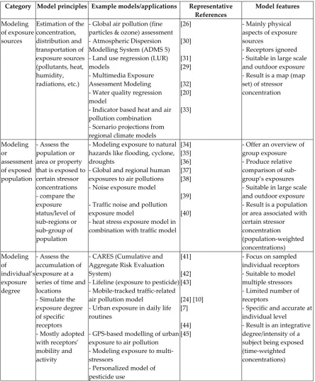
exposure consequences (integrated in Table 1). In this section each of these basic types of exposure
115
model are briefly described, along with inherent strengths or weaknesses, following with an analysis
116
of the gaps and capacities of an agent-based model.
117
2.1 Modeling of exposure sources
118
The modelling techniques adopted in current exposure models have evolved along distinct lines
119
for the various types of source [22]. An elementary step towards a modelling assessment of the
120
exposure to new compounds or pollutants (chemicals, materials) is to estimate their environmental
121
concentrations [23]. Most of these studies focusing on the concentrations of environmental risk factors
122
use mathematical models based on measurements extracted from a small number of fixed climatic
123
monitoring stations within indoor and outdoor urban types of environments [24]. Jerrett, et al. [25]
124
reviewed these models and sub-classified them as (i) proximity models, (ii) interpolation models, (iii)
125
land use regression models, (iv) dispersion models, and (v) integrated emission-meteorological
126
models. Geographical Information Systems (GIS) are often applied in these models to demonstrate
127
spatial and temporal patterns of environmental pollutants. Nevertheless, these kinds of models aim
128
to extrapolate the concentration distribution of the environmental stressors considering various
129
factors that affect patterns of distribution in the research area, mostly (part of) a city [26, and others
130
in Table 1].
131
Schnell, Potchter, Yaakov and Epstein [24] criticized such models: 1) they underestimate
132
concentrations of risk factors using limited monitoring measurements; 2) the complexity of pollutant
133
distribution patterns was hardly accurate in these models; and 3) the indoor environment was
134
ignored when using only outdoor monitoring data. Beyond Schnell’s criticism, these models mostly
135
focus on a single stressor of concern and describe a few pathways through which the receptor, either
136
a human or another organism, can be exposed [27]. However, awareness is growing that exposure to
137
single stressors is the exception rather than the rule [28]. In practice, organisms are often exposed to
138
multiple stressors, e.g., extreme weather, a chemical mixture or a combination of chemical, biological
139
and physical agents. Exposure to multiple stressors may take place concurrently or sequentially, and
140
the individual stressors may or may not interact [28].
141
To some extent, the effect of stressor concentrations cannot really be represented by exposure
142
models if there is no specified subject that suffers from the stressors. Moreover, due to raising
143
concerns of people-centered urban management, to date, the monitoring of urban environments has
144
not taken into account the dynamism of urban daily life [19]. Humans in the city are actively mobile
which influence greatly the consequence of individual exposures. Therefore, current studies intend
146
to combine the modeling of exposure sources with human and/or other exposed subjects [20,29].
147
Table 1. Selected sample models in studying human exposure to environmental stressors
148
Category Model principles Example models/applications Representative References
Model features
Modeling of exposure sources
Estimation of the concentration, distribution and transportation of exposure sources (pollutants, heat, humidity, radiations, etc.)
- Global air pollution (fine particles & ozone) assessment - Atmospheric Dispersion Modelling System (ADMS 5) - Land use regression (LUR) models
- Multimedia Exposure Assessment Modeling - Water quality regression model
- Indicator based heat and air pollution combination - Scenario projections from regional climate models
[26] [30] [31] [29] [32] [20] [33]
- Mainly physical aspects of exposure sources
- Receptors ignored - Suitable in large scale and outdoor exposure - Result is a map (map set) of stressor concentration Modeling or assessment of exposed population
- Assess the population or area or property that is exposed to certain stressor concentrations - compare the exposure status/level of sub-regions or sub-group of population
- Modeling exposure to natural hazards like flooding, cyclone, droughts
- Global and regional human exposures to air pollutions - Noise exposure model
- Traffic noise and pollution exposure model
- heat stress exposure model in combination with traffic model
[34] [35] [36] [37] [38] [39] [40]
- Offer an overview of group exposure - Produce relative comparison of sub-group’s exposures - Suitable in large scale and outdoor exposure - Result is a population or area associated with certain stressor concentration (population-weighted concentrations) Modeling of individual’s exposure degree
- Assess the accumulation of exposure at a series of time and locations
- Simulate the exposure degree of specific receptors - Mostly adopted with receptors’ mobility and activity
- CARES (Cumulative and Aggregate Risk Evaluation System)
- Lifeline (exposure to pesticide) - Mobile-tracked traffic-related air pollution model
- Urban exposure in daily life routines
- GPS-based modelling of urban exposure to air pollution - Modeling exposure to multi-stressors
- Personalized model of pesticide use [41] [42] [43] [24] [10] [7] [44] [45]
- Focus on sampled individual receptors - Suitable to model multiple stressors - Limited number of receptors
- Specific and accurate at individual level
- Result is an integrative degree/intensity of a subject being exposed (time-weighted concentrations)
2.2 Modeling of population exposure
149
Models of population exposure go a step further than the stressor concentration models do.
150
These models generally assess the size of a population, the area and/or property that is exposed to
151
certain stressor concentrations, and may also compare the exposure level of regions or
sub-152
groups (Table 1). Natural hazards like flooding, sea level rise, snow avalanches, droughts are among
153
the mostly targeted exposure sources. For example, the nation-wide exposure assessment in Austria
154
covers river flooding, torrential flooding, and snow avalanches [35]. A mapping study of flood
exposure detected flood inundation areas and the affected people [46], which indicated that exposure
156
depends strongly on the temporal and spatial dynamics of the distributed population. A few studies
157
also estimated global exposure to floods and revealed the economic exposure, population exposure
158
and geographical distribution of regional exposures [34,47,48]. Overall, these modeling approaches
159
help identifying highly exposed regions and are an important and suitable tool to inform regional or
160
nation-wide adaptation. Also the impact of the structure and morphology of cities on heat stress
161
exposure of urban commuters has been investigated by combining a simple heat stress model with a
162
traffic model that can track certain groups of commuters [40].
163
Population exposure models have been widely applied to explore human exposure to air
164
pollutions. Hystad, Setton, Cervantes, Poplawski, Deschenes, Brauer, van Donkelaar, Lamsal, Martin,
165
Jerrett and Demers [36] created national pollutant models to produce estimates of population
166
exposure to five common air pollutants (PM2.5, NO2, benzene, ethylbenzene, and butadiene) in
167
Canada. Global and regional exposure to black carbon [37], metals [49] and ozone [26] were also
168
estimated using similar approaches. Besides, a noise exposure model for London indicated that over
169
1 million residents were exposed to high daytime and night-time noise levels [38]. Modeling of traffic
170
pollution exposure in Toronto revealed the highest polluted areas and periods along roadways at
171
peak levels of traffic but the highest population exposure in the central business district due to the
172
higher population density [39].
173
Population exposure models often place strong emphasis on the geographical distribution of
174
populations, stressors and their estimated level or intensity of exposure, which might be called
175
population-weighted stressor concentrations [37]. These models have advantages in identifying
176
geographic areas, usually larger than a city, where hotspot exposures are a potential risk to human
177
health, and are informing decision making to reduce exposure inequalities [49]. New developments
178
in sensor technology now enable us to monitor multiple stressors and personal exposures in activity
179
spaces and fields of varying concentration [16].
180
2.3 Modeling of individual’s exposure degree
181
Individual exposure models simulate the exposure level of each receptor based on their
182
individual characteristics and within a pre-set specific route and/or space (Table 1). These approaches
183
were often seen in mobility-related exposure studies using empirical or experimental traffic data for
184
specific individuals [43,50]. Leyk, et al. (2009), presenting a spatial individual-based model prototype
185
for assessing potential pesticide exposure of farm-workers with their individual level track of
186
movement and activities. Similarly, more complex modeling tools were developed for quantification
187
of human exposure to traffic-related air pollution within distinct micro-environments by using GPS
188
trajectory analysis of the individuals in the city area [10,24]. Findings of these approaches show the
189
exposure of people to environmental sources of discomfort while performing their daily life activities
190
[7,10]. These studies suggested a shift from measuring environmental conditions in fixed monitoring
191
stations to monitoring with mobile portable sensors [44,51].
192
Individual exposure models were applied in both human models and wildlife models. Loos,
193
Schipper, Schlink, Strebel and Ragas [28] compared five human and five wildlife receptor-oriented
194
exposure models and identified their similarities regarding exposure endpoints, chemical stressors
195
and the extent of model validation, as well as the differences relate to the simulation of behavior and
196
the representation of individuals and space. In addition, an individual receptor can be considered as
197
an integrator of different stressors to which it is exposed while moving through space and time.
198
Therefore, exposure models for multiple stressors should primarily focus on the receptor, and not on
199
the stressor(s). A few studies have indeed reported the applicability of individual-oriented models in
200
modeling noise, black carbon, particle number concentrations, and multiple chemicals [41,44].
201
The assessment of individual exposure often aims to tell the total exposure degree or intensity
202
with a process of moving in different space sites. Sampling approaches are generally applied to collect
203
exposure data at different location and time, often along a planned routine in a city. The assessment
204
shows the consequence of accumulated exposure degree that is often a function of the stressor
205
concentration and the duration of being exposed, or so called time-weighted concentrations [52]. As
indicated in table 2, most individual exposure models don’t consider human exposure as a dynamic
207
process but as a summary over several time points/periods. This may be discussable in case of long
208
time continuing environment threats, for example, a heat wave that lasts several days. In practice,
209
monitoring of individual exposure is limited to studies with a small number of individuals because
210
of the high costs and complex organization associated with the measurements [10,51]. The results are
211
very much accurate and reliable at personal level, though they don’t show a big picture of the
212
exposure pattern of the whole city or area.
213
2.4 Research gaps and capacities of agent-based modelling
214
As shown above, dozens of studies have measured the concentrations of numerous stress
215
sources in different media to which humans are exposed. Others have catalogued the various
216
exposure pathways and identified the duration and accumulation of exposure for the general
217
population. All of this information allows better estimates of exposure. However, literature reviews
218
have demonstrated that the role of individual mobility for exposure was less explored and based on
219
limited monitoring data of personal samples [19]. The relationship between individual heterogeneity
220
and uniform group patterns, especially for peak exposure in “hot-spots” is still insufficiently
221
addressed and the contribution of mobility-related exposure is not clear [7]. In addition, the dynamic
222
process of changing exposure to various individuals requires innovative models that can identify the
223
emerging non-linear patterns of collective exposures. We hypothesize that a computer simulation
224
tool with a large number of individual random activities in different types of environments can
225
provide a better understanding of the consequences of human exposure to environmental risk factors
226
throughout the concerned space and time range.
227
To fill the research gaps and test the hypothesis, we recommend the development of an overall
228
framework for exploring the spatial and temporal variability of individual exposure concentrations
229
and emerging collective exposure patterns, a screening tool for exposure source concentrations, the
230
collection of better source and receptor data, the demonstration of exposure processes and collective
231
exposure patterns. While a few researchers have mentioned similar ideas taking into account activity
232
spaces and daily mobility in measuring environmental exposures [7,19,53], the present study is a
233
practical effort to implement them. An agent-based model (ABM) is a suitable tool to implement such
234
dynamic non-linear and collective simulations, as reviewed in existing studies on coupled
human-235
nature systems [54].
236
An agent-based model considers the essential known and measurable aspects of an agent and
237
acknowledges the nonlinearities and underlying dynamic processes [54-57]. An agent-based
238
approach can make an important contribution to improving health and wellbeing, both at individual
239
and collective group levels. In an ABM, agents are described by self-contained computer programs
240
that interact with its environment and with one another and can be designed and implemented to
241
describe rule-based behaviors and modes of interaction of observed social entities [55,58,59].
242
Regarding the field of environmental exposure studies, ABMs have the advantage to simulate
243
the exposure consequences of individual activities and the patterns of collective group exposures,
244
thus to suggest exposure reduction strategies accordingly. Currently, there is limited understanding
245
of the complex mobility exposure to environmental stresses in the specific urban context. There is an
246
urgent need to develop an innovative and operational approach to understanding urban health and
247
wellbeing that integrates individual characters within a mobility context. This, in turn, will help to
248
integrate substantive consideration of individual wellbeing into long-term planning, development
249
and management of urban environments. Exposure estimates to atmospheric pollutants can address
250
individuals (personal exposure) or large population groups (population exposure) and can be based
251
on direct (exposure monitoring) or indirect methods (exposure modelling). Efforts aiming at
252
providing useful global models have given rise to freely available, web-based databases, each acting
253
as a collector of the different data and models representing geophysical and meteorological risks.
3 An agent-based modelling framework
257
An agent-based prototype model to urban environment stresses is developed in the present
258
work for quantification of human exposure within distinct microenvironments and a novel approach
259
based on daily routine analysis of individuals. Subsequent sections provide the context on the model
260
environment and its implications for health, and outline a conceptual framework for the study of
261
health and wellbeing in and between urban spaces. Finally, guidance on research criteria and the use
262
of a systems approach is offered to prospective investigators for the development of research
263
proposals.
264
3.1 Model structure
265
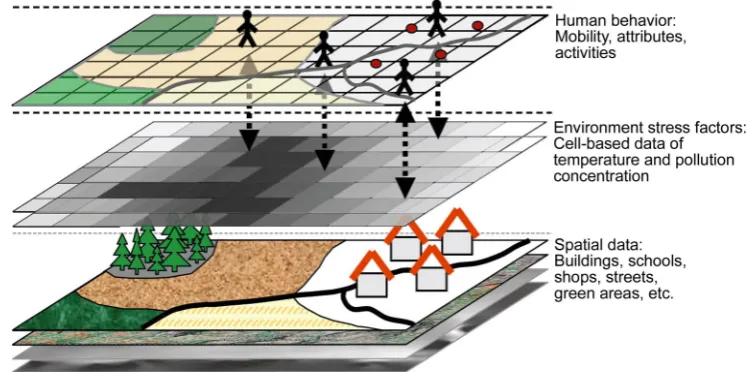
The model framework is structured in three overlapping layers: spatial data of the concerned
266
urban environment, concentrations of environmental stress sources, and human activities. Figure 1
267
illustrates the ABM used in this paper.
268
269
Figure 1. Illustration of the agent-based model framework for environmental exposure simulation. Applied
270
and illustrated based on Leyk, Binder and Nuckols [45]
271
In this framework, spatial data of the changing concentration patterns of the environmental
272
stress factors are the key pre-set inputs that build up the natural aspects of the system (center layer
273
in Figure 1). A specific map will be used to represent the city with buildings, streets, shops, green
274
areas, etc. (lower layer in Figure 1). Agents with initiated attributes act daily to work, rest, entertain,
275
shop, take care of children, and follow certain paths to work (top layer in Figure 1). Once the
276
prototype model is initialized, agents act on their daily life according to predetermined rules that are
277
set according to empirical studies and specific surveys. Depending on their normal lifestyles
278
(different among agents) as well as the environment stress factors of their location, they suffer or
279
reduce exposure levels. A simulation during a heat wave or air pollution event, with a period from
280
hours to days, would report a cumulative exposure level for each agent and a collective pattern of all
281
agents in the study area. The loops of agents’ daily activities and the evolution of the stressful factors
282
drive the model to run step by step, so that the exposure process can be analyzed. Finally, the model
283
produces summary information that can be used to diagnose both individual and collective exposure
284
and inform relevant exposure reduction strategies. Further details of the model components are
285
introduced in the following sections.
286
3.2 Modeling environment
287
The modeling environment includes two parts, the natural environment of the studied city area
288
and the stressed environment of a heat wave or air pollution event. The natural environment of the
289
city is represented by an integrated computable map of land-use data, street and building
290
information, key sites, and so on. Such data are usually available in GIS format.
In addition to data from the urban environment, geospatial data for the stressed environment
292
are needed to map the impact on agent movements. Environmental stressors such as high
293
temperatures or air pollution can be taken from measurements or from atmospheric model
294
simulations. These are usually gridded datasets with a fixed spatial resolution. The temporal
295
resolution typically varies between minutes and several hours. For simulating the exposure to
296
stressors both high spatial and temporal resolutions are desired. However, there are limits set by the
297
availability of observations, by the resolution of the models or the computing resources (e.g. disk
298
space, working memory or computing time).
299
The introduced modelling framework aims to simulate the exposure to air pollution and heat
300
stress in an urban area. Air pollution is elevated in urban areas mainly due to emissions from traffic
301
(fossil fuel driven vehicles and ships), industry and residential heating. Therefore, high
302
concentrations can be expected near big roads, harbor and industry areas. Pollutants range from
303
larger particles such as particular matter (PM) to gases such as Ozone, NOx, CO, etc. Most of them
304
are formed after several chemical reactions. Hence, chemistry models are applied to simulate the
305
concentration levels within urban areas [60]. The emissions of chemicals, which are crucial for the
306
chemistry model, are usually estimated from traffic, census, and monitoring stations.
307
It is well known that due to the heterorganic surfaces and three-dimensional structures (e.g.
308
buildings, trees, bridges etc.) temperatures and heat stresses can vary strongly within a city [61]. At
309
night-time the so called urban heat island (UHI) can develop for low wind speed and cloud cover
310
[62]. The UHI refers to higher near-surface temperatures in urban areas compared to the rural
311
surroundings. Also during the day temperatures are varying within the city. Especially, green and
312
blue areas (e.g. parks, lakes, rivers, etc.) have a cooling effect during the day. Since humans do feel
313
the environment as a combination of the meteorological variables temperature, humidity, wind speed
314
and long- and shortwave radiation, rather than temperature alone so-called biometeorological
315
indices are computed, which summarize the combined effect of the thermal environment on the
316
human heat budget of a person [63]. The developed prototype uses artificial temperature data
317
randomly chosen from a typical temperature range for Hamburg to validate the model because
high-318
resolution daily or hourly temperature or heat stress data for Hamburg are only available for periods
319
with a length of 3-4 days in summer [64,65].
320
3.3 Agent attributes and behaviors
321
The urban population is quite diverse, consisting of people of different ages, gender, living and
322
working location, social background, lifestyles etc. Hence, they all show a unique behavior.
323
Modelling each urban dweller of a city like Hamburg with 1.7 million citizens is not feasible due to
324
computing constraints and more importantly due to the lack of available data. However, it is possible
325
to group people with similar attributes and behaviors to agent types based on surveys, traffic data
326
and data from public transport companies. The behavior of urban dwellers can depend on age,
327
gender, work, income, education, living and work location, access to cars or public transport, and
328
environmental conditions (e.g. rain, temperature, and pollution levels). Crowd-sourcing information
329
on detailed time-location data can also be collected for each individual at each moment by
GPS-330
equipped mobile phones, offering many advantages over traditional time-location analysis, such as
331
high temporal resolution and minimum reporting burden for participants.
332
3.4 Daily routines
333
As mentioned before, agents have goals that they are following. These could be to go to work
334
every day, to take children to school or day care, etc. To facilitate the modeling, it is hypothesized
335
that the daily routine of a certain group of agents is uniform. This makes it possible to simulate as
336
many agent types as determined in grouping processes. According to the grouping properties of the
337
agents, the empirical data and survey data are used to generate synthetic daily routines, with agent
338
priorities for each option of the population commuting between different directions. To capture
339
variability in the travel survey and uncertainties in behavior, the synthetic daily routines can be
340
described as action probabilities or priorities p. An example of a synthetic daily routine for a female
agent, employed and aged 30-45 with one child is shown in Figure 2. In this example, the agent starts
342
the day at 8 am with standard deviation of 15 min. They then travel, via school to drop their children
343
off, to work with a 0.2 probability of visiting the shops for a while on route and so on. Parts of this
344
daily routine can be different among agents of the group, e.g. the staying time in a shop, but agents
345
in this group all have to visit such many places on the route.
346
347
348
Figure 2. Example of a daily routine for a female agent, employed, aged 30-45 with one child
349
4 Model implementation and results
350
In order to demonstrate the applicability of the ABM framework a prototype model
351
implemented in the Netlogo platform is set-up for the city of Hamburg which simulates the exposure
352
to air pollution of different kinds of agents living near the city center during their commute to work
353
(Figure 3). A detailed description is given in Rühe [66]. In the following, the employed data (Section
354
4.1), the agent types (Section 4.2), and the model formulation (Section 4.3) are described briefly. In
355
addition, some first results are presented (Section 4.4).
356
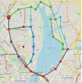
Figure 3. Map of commuting routes from home location (red house on the right) to work location (big red
357
house in top left corner) implemented in NetLogo. The third small house represents day nursery. Each note
358
use. The different colors represent the means of transport (blue=car, green=bike, yellow=public transport). For
360
car and bike different routes are possible indicated by the different shades of blue and green.
361
4.1 Data preparation for the case city of Hamburg
362
In the present model, NO2 concentration data are taken from model results from chemistry
363
transport model CityChem (Ramacher et al., 2017). The data are averaged for the summer and winter
364
of 2012 on a 250 m × 250 m grid. Values for temperature are taken from the DWD (German
365
Meteorological Service) and are randomly set at the same grid using typical ranges for summer (17 –
366
24.9 °C) and winter (0 – 8.9 °C). As soon as long-term high-resolution temperature or heat stress data
367
are available, they can be implemented with the same input routine used for the N02 data. For
368
simplicity the routes as well as the home and work locations are predefined (Figure 3 and Table 2).
369
Information about the costs for taking the car were taken from ADAC (Allgemeine Deutsche
370
Automobil-Club), information about bike costs from the Federal Environment Agency
371
(Umweltbundesamt) and the costs for public transportation in Hamburg were taken from the public
372
transportation service of Hamburg, HVV homepage (www.hvv.de). With this information it is
373
possible to calculate overall costs for each path.
374
Table 2. Time, length and costs for the different routes.
375
Car1 Car2 Car3 Car4 Car5 Bike Public Time [min] 10 16 17 15 13 19 18 Length [km] 5.1 5.3 6.8 7.1 6.6 5.0 6.3 Costs [€] 1.53 1.59 2.04 2.13 1.98 0.4 1.07
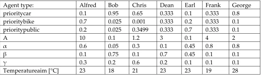
4.2 Settings of agents
376
The agent types are characterized by their different initial priorities for car, bike and public
377
transport (p1, p2, and p3), their different weights for costs, time, temperature deviation, exposure (α,
378
β, and γ), adaptation rate A and desired temperature Tdesired(Table 3). The values are set for typical
379
urban dwellers. Therefore, artificial values are used to create meaningful citizens. This work tries to
380
represent a broader cross section of society. This is why agent types reach from college students with
381
small amounts of money available, with high weights for costs and a high priority for bike
382
transportation, to old retired people with low weights for costs and with high priority for car
383
transportation.
384
Table 3. Attributes of different agents.
385
Agent type: Alfred Bob Chris Dean Earl Frank George
prioritycar 0.1 0.95 0.65 0.333 0.1 0.333 0.8 prioritybike 0.7 0.025 0.001 0.333 0.2 0.333 0.1 prioritypublic 0.2 0.025 0.3499 0.333 0.7 0.333 0.1
A 10 0.1 1.2 3 0.1 4 2
α 0.6 0.05 0.3 0.1 0.45 0.8 0.8
β 0.1 0.75 0.1 0.7 0.45 0.1 0.1
γ 0.3 0.2 0.6 0.2 0.1 0.1 0.1
Temperatureaim [°C] 23 18 21 23 23 19 28
4.3 Model formulation
386
In the model, agents are commuting to work using different means of transport (i.e. car, bike
387
and public transport) as well as different routes, where they are exposed to different air pollution
388
and temperature levels. The decision on which mean of transport to use is based on the priority p for
389
the k different choices while the change of the priorities is based on a value function v which in our
390
case is the weighted sum of commuting costs cc, commuting time ct, deviation from a desired
temperature dt (|T-Tdesired|) and the accumulated exposure to NO2eNO2 (Eq. 1). An exposure to NO2
392
occurs if a threshold of 30 µg/m³ is reached.
393
394
, ≤ 0
395
396
, = − + + + (1)
397
The parameter α, β, and γ represents the relevance of each term, which can differ between the
398
agents. The sum of all three parameters is 1. In order to make the different terms comparable they are
399
normalized with respect to their maximum and minimum. Hence, values can range from 0 to 1. For
400
simplicity the normalized exposure to high/low temperatures and the exposure to NO2 are combined
401
into one exposure term in the current version of the model. This means that they are currently equally
402
weighted because it is not yet clear how to combine the effect of exposure to both stressors on the
403
health of the agents.
404
Following Scheffran and BenDor [67] the change in priority is computed using Eq. (2).
405
∆ , = ∙ , ,
∑ ; ,∙ ,
∑ ; , (2)
406
where ai is the adaption parameter of agent i representing how fast an agent adapts and reacts
407
to changes. After each time step new priorities are computed (Eq. 3).
408
, ( ) = , ( − 1) + ∆ , ( − 1) (3)
409
The values for the exposure are computed during the model run while the values for costs and
410
the commuting time are currently predefined.
411
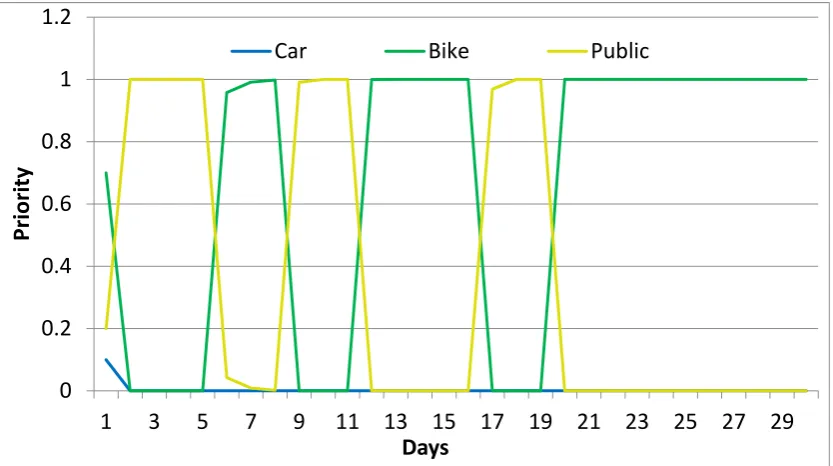
4.4 Preliminary results
412
In the developed model several model runs were conducted starting with model validation runs,
413
where “extreme” agents (e.g. setting α=1, β=0, and γ=0) are used to test for consistency and
414
plausibility. Afterwards, runs under simple conditions for all agents is executed followed by one runs
415
with low costs for public transportation, runs where rain is turned on, where a construction is
416
blocking one road and runs where the effect of NO2 in summer and winter is analyzed. The prototype
417
model is integrated for 120 days keeping the environmental conditions. It is obvious that a rain event
418
strongly affects the agents with a high prioritybike. Once a switch to public transport occurs (Figure 4),
419
this has a negative effect on the agents’ capital because costs for public transport are much higher
420
than for bike. Agents with highest priority for cars are not affected at all.
421
422
423
Figure 4. Changes in priorityi,k if rain is turned in and off for the agent Alfred.
424
0
0.2
0.4
0.6
0.8
1
1.2
1
3
5
7
9
11
13
15 17
19
21
23
25
27
29
Priority
Days
425
426
427
Figure 5. Changes in exposure to environmental stressors if a construction is blocking one path.
428
429
430
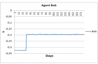
Figure 6. Changes in v if a construction is blocking one path.
431
432
A construction does only affect agents who are taking the car because one choosable path is not
433
available anymore. A construction does not affect the exposure to environmental stressors significant
434
but the commuting time. In Figure 5, it is visible that changes in exposure to environmental stressors
435
are not significant for Agent Bob, who has a high priority for car (Table 4). On the other hand, Figure
436
6 shows that a strong change in v (Eq. 2) occurs due to a decreasing commuting time.
439
440
Figure 7. Exposure to environmental stressors in summer (a) and winter months (b) for all agents.
441
442
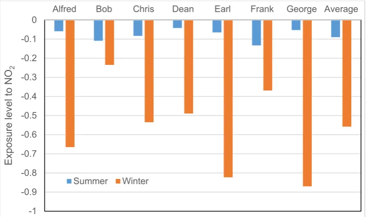
The differences in NO2 concentration in winter and summer have a significant effect on exposure
443
to environmental stressors (Figure 8). Several studies show that NO2 concentration is higher in winter
444
than in summer [68] mainly caused by more heating processes in winter months. In the first run
445
temperature is constant but to analyze the effect of heat stress varying temperatures are introduced.
The model shows that 42.5 °C must be reached to have the same exposure to temperature and NO2
447
in winter and summer. Based on pervious temperature measurements by the German Meteorological
448
Service (DWD) it is very unlikely to reach this value in Hamburg (highest temperature ever recorded
449
at Hamburg-Fuhlsbüttel: 37.3 °C). Figure 8 lists the average exposure to heat stress using the NO2
450
data for summer and winter. To sum it up, even the highest temperatures in Hamburg are not high
451
enough to show the same exposure effect than the high NO2 concentrations in winter months.
452
However, these simulations are idealized and it is not yet clear how to compare air pollution and
453
heat stress exposure directly e.g. with respect to health or wellbeing. Nevertheless, with the proposed
454
ABM both stressors can be modeled and assessed in a consistent way.
455
456
457
Figure 8. Individual and average normalized exposures to NO2 for summer and winter
458
5 Conclusion and outlooks
459
This paper presented an agent based modeling framework for dynamic micro-simulations of
460
urban individual exposures to environmental stresses. Using the framework for the Hamburg
461
scenario it is shown that it is flexible enough to handle a variety of input data and extend or replace
462
algorithms. For example, heat stress data from model results could be employed, which will become
463
available in the future.
464
Moreover, it is well possible to extend the prototype model. Therefore, extra algorithms should
465
be added to each package to verify, manipulate, add or delete data items according to the purpose of
466
the algorithm. Since for each new scenario different algorithms have to be used or implemented, it is
467
of great interest that algorithms should be clearly separated from the data structure. They also should
468
be easily exchangeable by others. The order in which algorithms are called should be flexible as well.
469
The algorithms are collected into a sub-package of that data structure which they manipulate.
470
It has been argued that traditional validation methods are less appropriate for agent-based
471
models, as by their very nature, such models are simplified representations of complex reality and
472
indicate what may happen rather than what will necessarily happen. This caveat notwithstanding,
473
the validity of this model has been considered in several ways as illustrated in the modeling
474
framework and implementation sections. Nevertheless, it is only a framework. The algorithms
475
presented for modeling are basic. Resources are needed to enhance those algorithms and to validate
476
the resulting demand against behavioral issues. Within the UrbMod project (von Szombathely et al.
477
2017) data from a stakeholder survey with a focus on daily routines of urban residents in Hamburg
478
(von Szombathely et al. 2018) and from the patients’ database at the University Hospital
Hamburg-479
Eppendorf are collected which can be used to set more realistic values for the attributes of the agents.
480
In addition, with respect to the heat stress exposure the individual differences of the agents (age,
481
gender) and their thermal history (e.g. time spend in sunshine) could be taken into account to model
482
-1 -0.9 -0.8 -0.7 -0.6 -0.5 -0.4 -0.3 -0.2 -0.1 0
Alfred Bob Chris Dean Earl Frank George Average
Exposure level
to
NO
2
personal dynamic thermal indices, similar to Bruse [69] but for a much larger domain and period. In
483
this way, the adaptive actions of an agent are linked with the exact thermal history experienced.
484
The purpose of this case study is not to simulate exact prediction of environmental events but to
485
demonstrate the utility and potential of an agent-based model to be used in an exposure analysis to
486
support environmental incident management. The conceptual approach in its current state relies on
487
simplified assumptions and interrelationships between the social and the environmental subsystem,
488
as well as artificial input data. This was necessary since real data are lacking and the complexity had
489
to be limited. The main objective, however, was to test feasibility of this approach for exposure
490
assessment and to fully understand the relevant mechanisms needed by developing a model
491
prototype. This work also shows the importance of interaction between the transportation
492
community and computer scientists. To satisfy the requirements concerning data management, data
493
processing, computational design and implementation, runtime issues, etc., it is necessary to include
494
computer knowledge into the transportation research process.
495
Acknowledgement: The authors thank Dejan Antanaskovic for preparation of the data. This work was
496
supported by the research project “Cities in Change - Development of a Multi-sectoral Urban
Development-497
Impact Model (UrbMod; LFF-FV17)”, a joint project of University of Hamburg, Hamburg University of
498
Technology, University Medical Center Hamburg-Eppendorf, Institute of Coastal Research at
Helmholtz-499
Zentrum Geesthacht, Max-Planck-Institute for Meteorology, and HafenCity University, funded by the State of
500
Hamburg.
501
Author Contributions: L. Emlyn Yang, Peter Hoffmann and Jürgen Scheffran designed the study; L. Emlyn
502
Yang did the literature overview and constructed the modeling framework; Sven Rühe performed the prototype
503
model for the Hamburg case; all authors contributed to write the paper.
504
Conflicts of Interest: The authors declare no conflict of interest.
505
506
References
507
1. IPCC. Managing the risks of extreme events and disasters to advance climate change adaptation. A special report of
508
working groups i and ii of the intergovernmental panel on climate change; Cambridge, UKand New York, NY,
509
USA, 2012; p 582.
510
2. Yang, L.; Scheffran, J.; Qin, H.; You, Q. Climate-related flood risks and urban responses in the pearl river
511
delta, china. Reg Environ Change 2015, 15, 379-391.
512
3. Kovats, R.S.; Hajat, S. Heat stress and public health: A critical review. Annual Review of Public Health 2008,
513
29, 41-55.
514
4. Lankao, P.R.; Qin, H. Conceptualizing urban vulnerability to global climate and environmental change. Curr
515
Opin Env Sust 2011, 3, 142-149.
516
5. Clausen, G.; Wyon, D.P. The combined effects of many different indoor environmental factors on
517
acceptability and office work performance. Hvac&R Res 2008, 14, 103-113.
518
6. Bai, X.M.; Nath, I.; Capon, A.; Hasan, N.; Jaron, D. Health and wellbeing in the changing urban environment:
519
Complex challenges, scientific responses, and the way forward. Curr Opin Env Sust 2012, 4, 465-472.
520
7. Dias, D.; Tchepel, O. Modelling of human exposure to air pollution in the urban environment: A gps-based
521
approach. Environ Sci Pollut Res 2014, 21, 3558-3571.
522
8. Evance, G. Environmental stress. Cambridge: Cambridge University Press: 1983.
523
9. von Szombathely, M.; Albrecht, M.; Antanaskovic, D.; Augustin, J.; Augustin, M.; Bechtel, B.; Bürk, T.;
524
Fischereit, J.; Grawe, D.; Hoffmann, P., et al. Conceptional modeling approach to health related urban
well-525
being. Urban sci. 1, 17. Urban Science 2017, 1, 17.
526
10. Schnell, I.; Potchter, O.; Yaakov, Y.; Epstein, Y.; Brener, S.; Hermesh, H. Urban daily life routines and human
527
exposure to environmental discomfort. Environmental Monitoring and Assessment 2012, 184, 4575-4590.
528
11. Rosenzweig, C.; Solecki, W.D.; Hammer, S.A.; Mehrotra, S. Climate change and cities: First assessment report of
529
the urban climate change research network. Cambridge University Press: 2011.
530
12. Kjellstrom, T.; Friel, S.; Dixon, J.; Corvalan, C.; Rehfuess, E.; Campbell-Lendrum, D.; Gore, F.; Bartram, J.
531
Urban environmental health hazards and health equity. Journal of Urban Health : Bulletin of the New York
532
Academy of Medicine 2007, 84, 86-97.
533
13. Silva, R.A.; West, J.J.; Zhang, Y.Q.; Anenberg, S.C.; Lamarque, J.F.; Shindell, D.T.; Collins, W.J.; Dalsoren, S.;
534
Faluvegi, G.; Folberth, G., et al. Global premature mortality due to anthropogenic outdoor air pollution and
535
14. UN. World urbanization prospects - the 2014 revision. Department of Economic and Social Affairs: New York,
537
2014.
538
15. Chan, M.; Solheim, E.; Taalas, P. Working as one un to address the root environmental causes of ill health.
539
Bulletin of the World Health Organisation 2017, 95, 2-2.
540
16. Steinle, S.; Reis, S.; Sabel, C.E. Quantifying human exposure to air pollution-moving from static monitoring
541
to spatio-temporally resolved personal exposure assessment. Science of the Total Environment 2013, 443,
184-542
193.
543
17. McGeehin, M.A.; Mirabelli, M. The potential impacts of climate variability and change on
temperature-544
related morbidity and mortality in the united states. Environmental Health Perspectives 2001, 109, 185-189.
545
18. Watson, A.; Bates, R.; Kennedy, D. Assessment of human exposure to air pollution: Methods, measurements,
546
and models. In Air pollution, the automobile, and public health, National Academies Press (US): Washington
547
(DC), 1988.
548
19. Yang, L.E.; Hoffmann, P.; Scheffran, J. Health impacts of smog pollution: The human dimensions of
549
exposure. The Lancet Planetary Health 2017, 1, e132-e133.
550
20. Willers, S.M.; Jonker, M.F.; Klok, L.; Keuken, M.P.; Odink, J.; van den Elshout, S.; Sabel, C.E.; Mackenbach,
551
J.P.; Burdorf, A. High resolution exposure modelling of heat and air pollution and the impact on mortality.
552
Environment International 2016, 89-90, 102-109.
553
21. Dhondt, S.; Beckx, C.; Degraeuwe, B.; Lefebvre, W.; Kochan, B.; Bellemans, T.; Panis, L.I.; Macharis, C.;
554
Putman, K. Health impact assessment of air pollution using a dynamic exposure profile: Implications for
555
exposure and health impact estimates. Environ. Impact Assess. Rev. 2012, 36, 42-51.
556
22. Fryer, M.; Collins, C.D.; Ferrier, H.; Colvile, R.N.; Nieuwenhuijsen, M.J. Human exposure modelling for
557
chemical risk assessment: A review of current approaches and research and policy implications.
558
Environmental Science & Policy 2006, 9, 261-274.
559
23. Gottschalk, F.; Scholz, R.W.; Nowack, B. Probabilistic material flow modeling for assessing the
560
environmental exposure to compounds: Methodology and an application to engineered nano-tio2 particles.
561
Environmental Modelling & Software 2010, 25, 320-332.
562
24. Schnell, I.; Potchter, O.; Yaakov, Y.; Epstein, Y. Human exposure to environmental health concern by types
563
of urban environment: The case of tel aviv. Environmental Pollution 2016, 208, 58-65.
564
25. Jerrett, M.; Arain, A.; Kanaroglou, P.; Beckerman, B.; Potoglou, D.; Sahsuvaroglu, T.; Morrison, J.; Giovis, C.
565
A review and evaluation of intraurban air pollution exposure models. J. Exposure Anal. Environ. Epidemiol.
566
2005, 15, 185-204.
567
26. Brauer, M.; Amann, M.; Burnett, R.T.; Cohen, A.; Dentener, F.; Ezzati, M.; Henderson, S.B.; Krzyzanowski,
568
M.; Martin, R.V.; Van Dingenen, R., et al. Exposure assessment for estimation of the global burden of disease
569
attributable to outdoor air pollution. Environmental Science & Technology 2012, 46, 652-660.
570
27. Ragas, A.M.J.; Oldenkamp, R.; Preeker, N.L.; Wernicke, J.; Schlink, U. Cumulative risk assessment of
571
chemical exposures in urban environments. Environment International 2011, 37, 872-881.
572
28. Loos, M.; Schipper, A.M.; Schlink, U.; Strebel, K.; Ragas, A.M.J. Receptor-oriented approaches in wildlife
573
and human exposure modelling: A comparative study. Environmental Modelling & Software 2010, 25, 369-382.
574
29. CEAM. Multimedia exposure assessment modeling. Epa center for exposure assessment modeling (ceam).
575
Https://www.Epa.Gov/exposure-assessment-models/multimedia; 2017.
576
30. CERC. Cambridge environmental research consultants (cerc), 2016. Atmospheric dispersion modelling system (adms
577
5) user guide, version 5.2. Cambridge. Uk; 2016.
578
31. Beelen, R.; Raaschou-Nielsen, O.; Stafoggia, M.; Andersen, Z.J.; Weinmayr, G.; Hoffmann, B.; Wolf, K.;
579
Samoli, E.; Fischer, P.; Nieuwenhuijsen, M., et al. Effects of long-term exposure to air pollution on
natural-580
cause mortality: An analysis of 22 european cohorts within the multicentre escape project. The Lancet 2014,
581
383, 785-795.
582
32. Bain, R.; Cronk, R.; Hossain, R.; Bonjour, S.; Onda, K.; Wright, J.; Yang, H.; Slaymaker, T.; Hunter, P.;
Prüss-583
Ustün, A., et al. Global assessment of exposure to faecal contamination through drinking water based on a
584
systematic review. Trop Med Int Health 2014, 19, 917-927.
585
33. Jones, B.; Oneill, B.C.; McDaniel, L.; McGinnis, S.; Mearns, L.O.; Tebaldi, C. Future population exposure to
586
us heat extremes. Nature Clim. Change 2015, 5, 652-655.
587
34. Jongman, B.; Ward, P.J.; Aerts, J.C.J.H. Global exposure to river and coastal flooding: Long term trends and
588
changes. Global Environ Chang 2012, 22, 823-835.
589
35. Fuchs, S.; Keiler, M.; Zischg, A. A spatiotemporal multi-hazard exposure assessment based on property data.
590
Nat Hazard Earth Sys 2015, 15, 2127-2142.
591
36. Hystad, P.; Setton, E.; Cervantes, A.; Poplawski, K.; Deschenes, S.; Brauer, M.; van Donkelaar, A.; Lamsal,
592
L.; Martin, R.; Jerrett, M., et al. Creating national air pollution models for population exposure assessment
593
37. Wang, R.; Tao, S.; Balkanski, Y.; Ciais, P.; Boucher, O.; Liu, J.F.; Piao, S.L.; Shen, H.Z.; Vuolo, M.R.; Valari,
595
M., et al. Exposure to ambient black carbon derived from a unique inventory and high-resolution model. P
596
Natl Acad Sci USA 2014, 111, 2459-2463.
597
38. Gulliver, J.; Morley, D.; Vienneau, D.; Fabbri, F.; Bell, M.; Goodman, P.; Beevers, S.; Dajnak, D.; Kelly, F.J.;
598
Fecht, D. Development of an open-source road traffic noise model for exposure assessment. Environmental
599
Modelling & Software 2015, 74, 183-193.
600
39. Amirjamshidi, G.; Mostafa, T.S.; Misra, A.; Roorda, M.J. Integrated model for microsimulating vehicle
601
emissions, pollutant dispersion and population exposure. Transportation Research Part D-Transport and
602
Environment 2013, 18, 16-24.
603
40. Hoffmann, P.; Fischereit, J.; Heitmann, S.; Schlünzen, K.H.; Gasser, I. Modeling exposure to heat stress with
604
a simple urban model. Urban Science 2018, 2, 9.
605
41. ILSI. Ilsi research foundation. Cumulative and aggregate risk evaluation system (cares) version 4.0
606
http://ilsirf.Org/wp-content/uploads/sites/5/2016/08/caresv4overview_install.Pdf. 2010.
607
42. LifeLine. Overview of the fundamentals of version 1.0 of lifeline - software for modeling aggregate and
608
cumulative exposures to pesticides. The lifeline™ project, september 2000. 2000.
609
43. Liu, H.Y.; Skjetne, E.; Kobernus, M. Mobile phone tracking: In support of modelling traffic-related air
610
pollution contribution to individual exposure and its implications for public health impact assessment.
611
Environmental Health 2013, 12.
612
44. Dekoninck, L.; Botteldooren, D.; Panis, L.I.; Hankey, S.; Jain, G.; Karthik, S.; Marshall, J. Applicability of a
613
noise-based model to estimate in-traffic exposure to black carbon and particle number concentrations in
614
different cultures. Environment International 2015, 74, 89-98.
615
45. Leyk, S.; Binder, C.R.; Nuckols, J.R. Spatial modeling of personalized exposure dynamics: The case of
616
pesticide use in small-scale agricultural production landscapes of the developing world. International Journal
617
of Health Geographics 2009, 8, 17-17.
618
46. Kwak, Y.; Park, J.; Arifuzzaman, B.; Iwami, Y.; Amirul, M.; Kondoh, A. In Rapid exposure assessment of
619
nationwide river flood for disaster risk resuction, XXIII ISPRS Congress, July 12-19, 2016, Prague, Czech Republic,
620
2016; The International Archives of the Photogrammetry, Remote Sensing and Spatial Information Sciences:
621
July 12-19, 2016, Prague, Czech Republic.
622
47. Neumann, B.; Vafeidis, A.T.; Zimmermann, J.; Nicholls, R.J. Future coastal population growth and exposure
623
to sea-level rise and coastal flooding - a global assessment. PLoS ONE 2015, 10.
624
48. Christenson, E.; Elliott, M.; Banerjee, O.; Hamrick, L.; Bartram, J. Climate-related hazards: A method for
625
global assessment of urban and rural population exposure to cyclones, droughts, and floods. Int. J. Env. Res.
626
Public Health 2014, 11, 2169-2192.
627
49. Caudeville, J.; Bonnard, R.; Boudet, C.; Denys, S.; Govaert, G.; Cicolella, A. Development of a spatial
628
stochastic multimedia exposure model to assess population exposure at a regional scale. Science of the Total
629
Environment 2012, 432, 297-308.
630
50. Jensen, S.S. Mapping human exposure to traffic air pollution using gis. Journal of Hazardous Materials 1998,
631
61, 385-392.
632
51. Gerharz, L.E.; Klemm, O.; Broich, A.V.; Pebesma, E. Spatio-temporal modelling of individual exposure to
633
air pollution and its uncertainty. Atmos Environ 2013, 64, 56-65.
634
52. Dons, E.; Van Poppel, M.; Panis, L.I.; De Prins, S.; Berghmans, P.; Koppen, G.; Matheeussen, C. Land use
635
regression models as a tool for short, medium and long term exposure to traffic related air pollution. Science
636
of the Total Environment 2014, 476, 378-386.
637
53. Perchoux, C.; Chaix, B.; Cummins, S.; Kestens, Y. Conceptualization and measurement of environmental
638
exposure in epidemiology: Accounting for activity space related to daily mobility. Health Place 2013, 21,
86-639
93.
640
54. An, L. Modeling human decisions in coupled human and natural systems: Review of agent-based models.
641
Ecological Modelling 2012, 229, 25-36.
642
55. Bonabeau, E. Agent-based modeling methods and techniques for simulating human systems. PNAS 2002,
643
99, 7280-7287.
644
56. Heppenstall, A.J.; Crooks, A.T.; See, L.M.; Batty, M. Agent-based models of geographical systems. Springer
645
Science & Business Media: 2011.
646
57. Langevin, J.; Wen, J.; Gurian, P.L. Simulating the human-building interaction: Development and validation
647
of an agent-based model of office occupant behaviors. Build. Environ. 2015, 88, 27-45.
648
58. Monticino, M.; Acevedo, M.; Callicott, B.; Cogdill, T.; Lindquist, C. Coupled human and natural systems: A
649
multi-agent-based approach. Environmental Modelling & Software 2007, 22, 656-663.
650
59. An, L.; Lopez-Carr, D. Understanding human decisions in coupled natural and human systems. Ecological