Article
1
Predicting motor insurance claims using telematics
2
data - XGBoost vs. logistic regression
3
Jessica Pesantez-Narvaez, Montserrat Guillen and Manuela Alcañiz
4
Dept. Econometrics, Riskcenter-IREA, Universitat de Barcelona; [email protected], (J.P-N)
5
https://orcid.org/0000-0003-3161-7807; [email protected] (M.G); https://orcid.org/0000-0002-2644-6268;
6
[email protected] (M.A) https://orcid.org/0000-0002-5028-1926
7
* Correspondence: [email protected]; Tel.: +34-934-037-039
8
9
Abstract:
10
XGBoost is recognized as an algorithm with exceptional predictive capacity. Models for a binary
11
response indicating the existence of accident claims vs. no claims can be used to identify the
12
determinants of traffic accidents. We compare the relative performances of logistic regression and
13
XGBoost approaches for predicting the existence of accident claims using telematics data. The
14
dataset contains information from an insurance company about individuals’ driving patterns –
15
including total annual distance driven and percentage of total distance driven in urban areas. Our
16
findings show that logistic regression is a suitable model given its interpretability and good
17
predictive capacity. XGBoost requires numerous model-tuning procedures to match the predictive
18
performance of the logistic regression model and greater effort as regards interpretation.
19
Keywords: dichotomous response; predictive model; tree boosting; GLM; machine learning
20
21
1. Introduction
22
Predicting the occurrence of accident claims in motor insurance lies at the heart of premium
23
calculation, but with the development of new artificial intelligence methods, the question of choosing a
24
suitable model has yet to be completely solved. In this article, we consider the recently proposed
25
methods of XGBoost (Chen and Guestrin 2016) and logistic regression and compare their predictive
26
performance in a sample of insured drivers, for whom we have telematic information.
27
We discuss the advantages and disadvantages of XGBoost compared to logistic regression and we
28
show that a slightly improved predictive power is only obtained with the XGBoost method, but this
29
complicates the interpretation of the impact of covariates on the expected response. In the case of
30
automobile insurance, where the premium calculation is regulated and has to be fully specified, the
31
weight of each risk factor in the final price needs to be disclosed and the connection between the
32
observed covariate value and the estimated probability of a claim needs to be shown. If these
33
conditions are not met, the regulating authority may deny the insurance company the right to
34
commercialize that product. We discuss, nevertheless, why the use of an XGBoost algorithm remains
35
interesting for actuaries and how methods both old and new might be combined for optimum results.
36
We do not examine any other boosting methods here and remind readers that excellent descriptions
37
can be found in Lee and Lin (2018), while extensions to high dimensional datasets are presented in
38
Lee and Antonio (2016), both of which present cases studies of insurance applications. Many of those
39
alternatives place their emphasis on algorithm speed, but in terms of their essential setups they do not
40
differ greatly from XGBoost.
41
To compare the two competing methods, we use a real dataset comprising motor insurance
42
policy holders and their telematics measurements, that is, real-time driving information collected and
43
stored via telecommunication devices. More specifically, GPS-based technology captures an insured’s
44
driving behavior patterns, including distance travelled, driving schedules, and driving speed, among
45
many others. Here, pay-as-you-drive (PAYD) insurance schemes represent an alternative method for
46
pricing premiums based on personal mileage travelled and driving behaviors. Guillen et al. (2019),
47
Verbelen et al. (2018), and Pérez-Marin and Guillen (2019) show the potential benefits of analyzing
48
telematics information when calculating motor insurance premiums. Further, Hultkrantz et al. (2012)
49
highlight the importance of PAYD insurance plans insofar as they allow insurance companies to
50
personalize premium calculation and, so, charge fairer rates.
51
The rest of this paper is organized as follows. First, we introduce the notation and outline the
52
logistic regression and XGBoost methods. Second, we describe our dataset and provide some
53
descriptive statistics. Third, we report the results of our comparisons in both a training and a testing
54
sample. Finally, we conclude and offer some practical suggestions about the feasibility of applying
55
new machine learning methods to the field of insurance.
56
2. Methodology description
57
Let us suppose that in a data set of n individuals and P covariates, we have a binary response
58
variable 𝑌, i= 1,…,n taking values 0,1; and a set of covariates denoted as 𝑋 , p=1,…,P. The
59
conditional probability density function of 𝑌 = t (t= 0,1) given 𝑋 (𝑋 , … , 𝑋 ), is denoted as ℎ (𝑋 ).
60
Equivalently, we say that Prob(Yi = t)=ℎ (𝑋 ), and that E(Yi )=Prob(Yi = 1)=ℎ (𝑋 ).
61
2.1. Logistic regression
62
Logistic regression, a widely recognized regression method for predicting the expected
63
outcome of a binary dependent variable, is specified by a given set of predictor variables. McCullagh
64
and Nelder (1989) presented the logistic regression model as part of a wider class of generalized
65
linear models. What distinguishes a logistic regression from a classical linear regression model is
66
primarily that the response variable is binary rather than continuous in nature.
67
The logistic regression uses the logit function as a canonical link function, in order words, the
68
log ratio of the probability functions ℎ(𝑋) is a linear function of X; that is:
69
𝑙𝑛 ( )( )= 𝑙𝑛Prob(Yi = 1)
Prob(Yi = 0)= 𝛽 + ∑ 𝑋 𝛽 , (1)
70
where 𝛽 , 𝛽 , . . . , 𝛽 are the model coefficients1, and Prob(Yi = 1) is the probability of observing the
71
event in the response (response equal to 1), and Prob(Yi = 0) is the probability of not observing the
72
event in the response (response equal to 0).
73
The link function provides the relationship between the linear predictor դ = 𝛽 + ∑ 𝑋 𝛽
74
and the mean of the response given certain covariates. In a logistic regression model, the expected
75
response is:
76
𝐸(𝑌 ) = Prob(Yi = 1) = ∑
∑ . (2)
77
A logistic regression can be estimated by maximum likelihood (for further details see, for example,
78
Greene 2002). Therefore, the idea underlying a logistic regression model is that there must be a linear
79
combination of risk factors that is related to the probability of observing an event. The data analyst’s
80
task is to find the fitted coefficients that best estimate the linear combination in (2) and to interpret
81
the relationship between the covariates and the expected response. In a logistic regression model, a
82
positive estimated coefficient indicates a positive association; thus, when the corresponding
83
covariate increases, the probability of the event response also increases. Correspondingly, if the
84
estimated coefficient is negative then the association is negative and, so, the probability of the event
85
decreases when the observed value of the corresponding covariate increases. Odds-ratios can be
86
calculated as the exponential values of the fitted coefficients and they can also be directly interpreted
87
as the change in odds when the corresponding factor increases by one unit.
88
1 Note we have opted to refer here to ‘coefficients’ as opposed to ‘parameters’ to avoid confusion with the
Apart from their interpretability, the popularity of logistic regression models is based on two
89
characteristics: (i) maximum likelihood estimates are easily found and (ii) the analytical form of the
90
link function in (2) always provides predictions between 0 and 1 that can be directly interpreted as
91
the event probability estimate. For these motives, logistic regression has become one of the most
92
popular classifiers, their results providing a straightforward method for predicting scores or
93
propensity values which, in turn, allow new observations to be classified to one of the two classes in
94
the response. For R users, the glm function is the most widely used procedure for obtaining
95
coefficient estimates and their standard errors, but alternatively a simple optimization routine can
96
easily be implemented.
97
2.2. XGBoost
98
Chen and Guestrin (2016) proposed XGBoost as an alternative method for predicting a response
99
variable given certain covariates. The main idea underpinning this algorithm is that it builds D
100
classification and regression trees (or CARTs) one by one, so that each subsequent model (tree) is
101
trained using the residuals of the previous tree. In order words, the new model corrects the errors
102
made by the previously trained tree and then predicts the outcome.
103
In the XGBoost, each ensemble model2 uses the sum of D functions to predict the output:
104
𝑌 = ₣(𝑋 ) = ∑ 𝑓 (𝑋 ) , 𝑓 𝜖 Ϝ, 𝑖 = 1, … , 𝑛 (3)
105
where Ϝ is the function space3 of the CART models, and each 𝑓 corresponds to an independent
106
CART structure which we denote as q. In other words, q is the set of rules of an independent CART
107
that classifies each individual i into one leaf. The training phase involves classifying n observations
108
so that, given the covariates X, each leaf has a score that corresponds to the proportion of cases
109
which are classified into the response event for that combination of 𝑋. We denote this score as
110
𝑤 ( ).
111
Thus, we can write q as a function q: ℝ T , where T is the total number of leafs of a tree and j
112
is later used to denote a particular leaf, j=1,…,T. To calculate the final prediction for each individual,
113
we sum the score of the leafs as in (3), where Ϝ = { f(X) = 𝑤 ( )}, with q: ℝ T, and 𝑤 𝜖 ℝ .
114
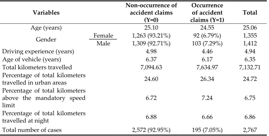
In general, boosting methods fit D models in D iterations (each iteration denoted by d, d=1,…,D)
115
in reweighted versions. Weighting is a mechanism that penalizes the incorrect predictions of past
116
models, in order to improve the new models. The weighting structures are generally optimal values,
117
which are adjusted once a loss function is minimized. Then new learners incorporate the new
118
weighting structure in each iteration, and predict new outcomes. In particular, the XGBoost method
119
minimizes a regularized objective function, i.e. the loss function plus the regularization term:
120
ℒ = ∑ ℓ 𝑌 , 𝑌 + ∑ ή(𝑓 ), (4)
121
where ℓ is a convex loss function that measures the difference between the observed response 𝑌
122
and predicted response 𝑌 and ή = µT+ 𝜆‖𝑤‖ , ή is the regularization term also known as the
123
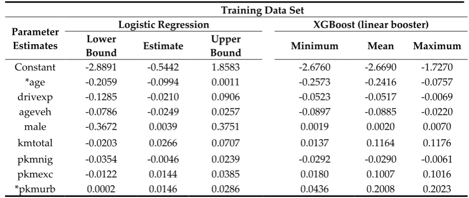
shrinkage penalty which penalizes the complexity of the model and avoids the problem of
124
overfitting. The tree pruning parameter µ regulates the depth of the tree and 𝜆 is the regularization
125
parameter that is associated with l2-norm of the scores vector, which is a way of evaluating the
126
magnitude of scores. Including this norm, or any other similar expression, penalizes excessive sizes
127
in the components of 𝑤.
128
Note that pruning is a machine learning technique which reduces the size of a decision tree by
129
removing decision nodes whose corresponding features have little influence on the final prediction
130
2 Natekin and Knoll (2013) explain that the ensemble model can be understood as a committee formed by a
group of base learners or weak learners. Thus, any weak learner can be introduced as a boosting framework. Various boosting methods have been proposed, including: (B/P-) splines (Huang and Yang 2004); linear and penalized models (Hastie et al. 2009); decision trees (James et al. 2013); radial basis functions (Gomez-Verdejo et al. 2002); and Markov random fields (Dietterich et al. 2008). Although Chen and Guestrin (2016) state 𝑓 as a CART model, the R package xgboost currently performs three boosters: linear, tree and dart.
3 The XGBoost works in a function space rather than in a parameter space. This framework allows the objective
of the target variable. This procedure reduces the complexity of the model and, thus, corrects
131
overfitting.
132
The l2-norm is used in the L2 or Ridge regularization method, while the l1-norm is used in the
133
L1 or Lasso regularization method. Both methods can take the Tikhonov or the Ivanov form (see
134
Tikhonov and Arsenin 1977; Ivanov 2003).
135
A loss function or a cost function like (4) measures how well a predictive algorithm fits the
136
observed responses in a data set (for further details, see Friedman et al. 2001). For instance, in a
137
binary classification problem, the logistic loss function is suitable because the probability score is
138
bounded between 0 and 1. Then, by selecting a suitable threshold, a binary outcome prediction can
139
be found. Various loss functions have been proposed in the literature, including: the square loss, the
140
hinge loss (Steinwart and Christmann 2008), the logistic loss (Schapire and Freund 2012), the cross
141
entropy loss (de Boer et al. 2015) and the exponential loss (Elliott and Timmermann 2013).
142
The intuition underpinning the regularization proposed in (4) involves reducing the magnitude
143
of 𝑤, so that the procedure can avoid the problem of overfitting. The larger the ή, the smaller the
144
variability of the scores (Goodfellow et al. 2016).
145
The objective function at the d-th iteration is :
146
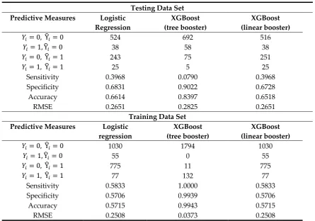
ℒ( )= ∑ ℓ 𝑌 , 𝑌( )+ 𝑓 (𝑋 ) + ή(𝑓 ), (5)
147
where 𝑌( )is the prediction of the i-th observation at the (d-1)-th iteration. Note that ℓ(·,·) is
148
generally a distance so its components can be swapped, i.e. ℓ 𝑌 , 𝑌 = ℓ 𝑌 , 𝑌 . Following Chen and
149
Guestrin (2016), we assume that the loss function is a symmetric function.
150
Due to the non-linearities in the objective function to be minimized, the XGBoost is an
151
algorithm that uses a second-order Taylor approximation of the objective function ℒ in (5) as
152
follows:
153
ℒ( )≅ ∑ [ ℓ 𝑌 , 𝑌( ) + 𝑔 𝑓 (𝑋 ) + ℎ 𝑓 (𝑋 )] + ή(𝑓 ), (6)
154
where 𝑔 =𝜕 ( ) ℓ 𝑌 , 𝑌( ) and ℎ = 𝜕 ( ) ℓ 𝑌 , 𝑌
( )
denote the first and second
155
derivatives of the loss function ℓ with respect to the component corresponding to the predicted
156
classifier.
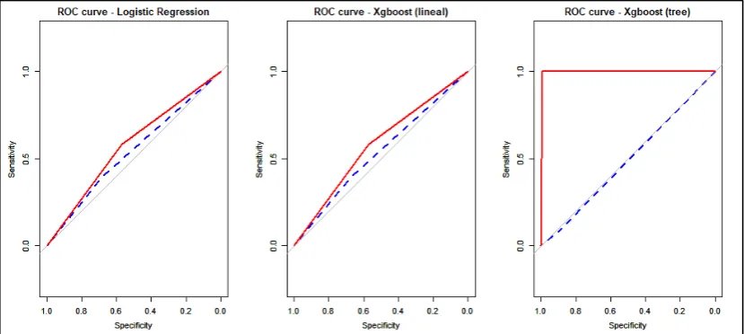
157
Since we minimize (6) with respect to 𝑓 , we can simplify this expression by removing constant
158
terms as follows:
159
ℒ( )= ∑ [𝑔 𝑓 (𝑋 ) + ℎ 𝑓 (𝑋 )] + ή(𝑓 ). (7)
160
Substituting the shrinkage penalty ή of (4) in (7), we obtain:
161
ℒ( )= ∑ [𝑔 𝑓 (𝑋 ) + ℎ 𝑓 (𝑋 )]+ µT+ 𝜆‖𝑤‖ . (8)
162
The l2-norm shown in (8) is equivalent to the sum of the squared weights of all T leafs.
163
Therefore (8) is expressed as:
164
ℒ( )= ∑ [𝑔 𝑓 (𝑋 ) + ℎ 𝑓 (𝑋 )]+ µT+ 𝜆 ∑ 𝑤 . (9)
165
Now, let us define 𝐼 = {i|q(𝑋)}, 𝐼 is the set of observations that are classified into one leaf j,
166
j=1,…,T. Each 𝐼 receives the same leaf weight 𝑤. So ℒ( )in (9) can also be seen as an objective
167
function that corresponds to each set 𝐼. In this sense, the 𝑓 (𝑋 ), which is assigned to the
168
observations, corresponds to the weight wj that is assigned to each set 𝐼. Therefore (9) is expressed
169
as:
170
ℒ( )= ∑ ∑є 𝑔 𝑤 + ∑є ℎ + 𝜆 𝑤 + µT. (10)
171
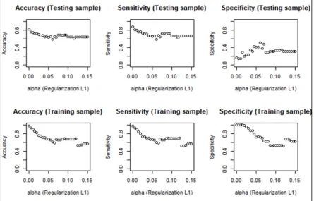
In order to find the optimal leaf weight 𝑤∗, we derive (10) with respect to 𝑤, let the new
172
equation be equal to zero, and clear the value of 𝑤∗. Then we obtain:
173
𝑤∗= −
∑
∑ . (11)
174
So we update (10) by replacing the new 𝑤∗. The next boosting iteration will minimize the following
175
objective function:
176
ℒ( )= ∑ ∑ 𝑔 −
∑
∑ + ∑ ℎ +𝜆 − ∑
∑ + µT =
= − ∑
∑
∑ + µ𝑇. (12)
178
Once the best objective function has been defined and the optimal leaf weights assigned to 𝐼,
179
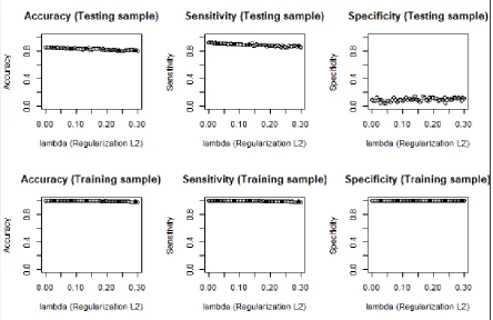
we next consider what the best split procedure will be. Because (12) is derived for a wide range of
180
functions, we are not able to identify all possible tree structures q in each boosting iteration. This
181
algorithm starts by building a single leaf and continues by adding new branches. Consider the
182
following example:
183
Let 𝐼 and 𝐼 be the sets of observations that are in the left and right parts of a node following a
184
split. So that I = 𝐼 + 𝐼 .
185
ℒ( )= − ∑
∑
∑ + ∑ ∑
∑ + ∑ ∑
∑ − µ , (13)
186
ℒ( )of (13) is the node impurity measure, which is calculated for the P covariates. The split is
187
determined by the maximum value of (13). For example, in the case of CART algorithms, the
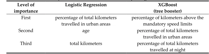
188
impurity measure for categorical target variables can be information gain, Gini impurity or
189
chi-square, while for continuous target variables it can be the Gini impurity.
190
Once the tree 𝑓 is completely built (i.e. its branches and leaf weights are established),
191
observations are mapped on the tree (from the root to one corresponding leaf). Thus, the algorithms
192
will update from (5) to (14) as many times as D boosting iterations are established and the final
193
classification is the sum of the D obtained functions which are shown in (3). Consequently, the
194
XGBoost corrects the mistaken predictions in each iteration, as far as this is possible, and tends to
195
overfit the data. Thus, to prevent overfitting, the regularization parameter value in the objective
196
function is highly recommended.
197
The implementation of XGBoost has proved to be quite effective for fitting real binary response
198
data and a good method for providing a confusion matrix, i.e. a table in which observations and
199
predictions are compared, with very few false positives and false negatives. However, since the final
200
prediction of an XGBoost algorithm is the result of a sum of D trees, the graphical representation and
201
the interpretation of the impact of each covariate on the final estimated probability of occurrence
202
may be less direct than in the linear or logistic regression models. For instance, if the final predictor
203
is a combination of several trees, but each tree has a different structure (in the sense that each time
204
the order of segmentation differs from that of the previous tree), the role of each covariate will
205
depend on understanding how the covariate impacts the result in the previous trees and what the
206
path of each observation is in each of the previous trees. Thus, in the XGBoost approach, it is difficult
207
to isolate the effect on the expected response of one particular covariate compared to all the others.
208
Under certain circumstances, the XGBoost method can be interpreted directly. This happens
209
when 𝑓 have analytical expressions that can easily be manipulated to compute ∑ 𝑓 (𝑋 ). One
210
example is the linear booster, which means that each 𝑓 is a linear combination of the covariates
211
rather than a tree-based classifier. In this case of a linear function, the final prediction is also a linear
212
combination of the covariates, resulting from the sum of the weights associated with each covariate
213
in each 𝑓 .
214
Results for the true XGBoost predictive model classifier can easily be obtained in R with the
215
xgboost package.
216
3. Data and Descriptive Statistics
217
Our case-study database comprises 2,767 drivers under 30 years of age who underwrote a
218
pay-as-you-drive (PAYD) policy with a Spanish insurance company. Their driving activity was
219
recorded using a telematics system. This information was collected from January 1 through to
220
December 31, 2011. The data set contains the following information about each driver: insured’s age
221
(age), age of the vehicle (ageveh) in years, insured’s gender (male), driving experience (drivexp) in
222
years, percentage of total kilometers travelled in urban areas (pkmurb), percentage of total kilometers
223
travelled at night – that is, between midnight and 6 am (pkmnig), the percentage of kilometers above
224
accident claim with fault (Y) which was coded as 1 when, at least, one claim with fault occurred in
226
the observational period and was reported to the insurance company, and 0 otherwise. We are
227
interested in predicting Y using the aforementioned covariates. This data set has been extensively
228
studied in Ayuso et al. (2014, 2016a, 2016b); and Boucher et al. (2017).
229
Table 1 shows the descriptive statistics for the accident claims data set. This highlights that a
230
substantial part of the sample did not suffer an accident in 2011, with just 7.05% of drivers reporting
231
at least one accident claim. Insureds with no accident claim seem to have travelled fewer kilometers
232
than those presenting a claim. The non-occurrence of accident claims is also linked to a lower
233
percentage of driving in urban areas and a lower percentage of kilometers driven above mandatory
234
speed limits. In this dataset, 7.29% of men and 6.79% of women had an accident during the
235
observation year.
236
Table 1. Description of the variables in the accident claims data set1
237
Variables
Non-occurrence of
accident claims (Y=0)
Occurrence of accident claims (Y=1)
Total
Age (years) 25.10 24.55 25.06
Gender Female 1,263 (93.21%) 92 (6.79%) 1,355
Male 1,309 (92.71%) 103 (7.29%) 1,412
Driving experience (years) 4.98 4.46 4.94
Age of vehicle (years) 6.37 6.17 6.35
Total kilometers travelled 7,094.63 7,634.97 7,132.71
Percentage of total kilometers
travelled in urban areas 24.60 26.34 24.72
Percentage of total kilometers above the mandatory speed limit
6.72 7.24 6.75
Percentage of total kilometers
travelled at night 6.88 6.66 6.86
Total number of cases 2,572 (92.95%) 195 (7.05%) 2,767
1The mean of the variables according to the occurrence and non-occurrence of accident claims. The absolute
238
frequency and row percentage is shown for the variable gender.
239
The data set is divided randomly into a training data set of 1,937 observations (75% of the total
240
sample) and a testing data set of 830 observations (25% of the total sample). Function
241
CreateDataPartion of R was used to maintain the same proportion of events (coded as 1) of the
242
total sample in both the training and testing data sets.
243
4. Results
244
In this section, we compare the results obtained in the training and testing samples when
245
employing the methods described in Section 2.
246
4.1. Coefficient Estimates
247
Table 2 presents the estimates obtained using the two methods. Note, however, that the values
248
are not comparable in magnitude as they correspond to different specifications. The logistic
249
regression uses its classical standard method to compute the coefficients of the variables and their
250
standard errors. However, the boosting process of the XGBoost builds D models in reweighted
251
versions and, so, we obtain a historical record of the D times P+1 coefficient estimates. XGBoost can
252
only obtain a magnitude of those coefficients if the base learner allows it, and this is not the case
253
when 𝑓 are CART models.
254
The signs obtained by the logistic regression point estimate and the mean of the XGBoost
255
coefficients are the same. Inspection of the results in Table 2 shows that, in general, older insureds
256
travel more kilometers in urban areas are more likely to have an accident than those that travel fewer
258
kilometers in urban areas. We are not able to interpret the coefficients of the XGBoost, but by
259
inspecting the maximum and minimum values of the linear booster case, we obtain an idea of how
260
the estimates fluctuate until iteration D.
261
Table 2. The parameter estimates of the logistic regression and XGBoost with linear booster.
262
Training Data Set
Parameter Estimates
Logistic Regression XGBoost (linear booster)
Lower
Bound Estimate
Upper
Bound Minimum Mean Maximum
Constant -2.8891 -0.5442 1.8583 -2.6760 -2.6690 -1.7270
*age -0.2059 -0.0994 0.0011 -0.2573 -0.2416 -0.0757
drivexp -0.1285 -0.0210 0.0906 -0.0523 -0.0517 -0.0069
ageveh -0.0786 -0.0249 0.0257 -0.0897 -0.0885 -0.0220
male -0.3672 0.0039 0.3751 0.0019 0.0020 0.0070
kmtotal -0.0203 0.0266 0.0707 0.0137 0.1164 0.1176
pkmnig -0.0354 -0.0046 0.0239 -0.0292 -0.0290 -0.0061 pkmexc -0.0122 0.0144 0.0385 0.0180 0.1007 0.1016 *pkmurb 0.0002 0.0146 0.0286 0.0436 0.2008 0.2023 In the logistic regression columns, the point estimates are presented with the lower and upper bound of a 95%
263
confidence interval. In the XGBoost columns, the means of the coefficient estimates with a linear boosting of the
264
D iterations are presented. Similarly, bounds are presented with the minimum and maximum values in the
265
iterations. There are no regularization parameter values. * Indicates that the coefficient is significant at the 90%
266
confidence level in the logistic regression estimation. Calculations were performed in R and scripts are available
267
from the authors.
268
Only the coefficients of age and percentage of kilometers travelled in urban areas are
269
significantly different from zero in the logistic regression model, but we have preferred to keep all
270
the coefficients of the covariates in the estimation results so as to show the general effect of the
271
telematics covariates on the occurrence of accident at-fault claims in this dataset, and to evaluate the
272
performance of the different methods in this situation.
273
274
Figure 1. The magnitude of all the estimates in the D=200 iterations.
275
Different colors indicate each of the coefficients in the XGBoost iteration.
276
Figure 1 shows the magnitude of all the estimates of the XGBoost in 200 iterations. From
277
approximately the tenth iteration, the coefficient estimates tend to become stabilized. Thus, no
278
extreme changes are present during the boosting.
279
The performance of the two methods is evaluated using the confusion matrix, which compares
281
the number of observed events and non-events with their corresponding predictions. Usually, the
282
larger the number of correctly classified responses, the better the model. However, out-of-sample
283
performance is even more important than in-sample results. This means that the classifier must be
284
able to predict the observed events and non-events in the testing sample and not just in the training
285
sample.
286
The predictive measures used to compare the predictions of the models are sensitivity,
287
specificity, accuracy and the root mean square error (RMSE). Sensitivity measures the proportion of
288
actual positives that are classified correctly as such, i.e. True positive/(True positive + False
289
negative). Specificity measures the proportion of actual negatives that are classified correctly as
290
such, i.e. True negative/(True negative + False positive). Accuracy measures the proportion of total
291
cases classified correctly (True positive + True negative)/Total cases. RMSE measures the distance
292
between the observed and predicted values of the response. It is calculated as follows:
293
∑ ( ) , (14)
294
The higher the sensitivity, the specificity and the accuracy, the better the models predict the
295
outcome variable. The lower the value of RMSE, the better the predictive performance of the model.
296
Table 3. Confusion matrix and predictive measures of the logistic regression, XGBoost with a tree booster and
297
XGBoost with a linear booster for the testing and training data sets.
298
Testing Data Set Predictive Measures Logistic
Regression
XGBoost (tree booster)
XGBoost (linear booster)
𝑌 = 0, Y = 0 524 692 516
𝑌 = 1, Y = 0 38 58 38
𝑌 = 0, Y = 1 243 75 251
𝑌 = 1, Y = 1 25 5 25
Sensitivity 0.3968 0.0790 0.3968
Specificity 0.6831 0.9022 0.6728
Accuracy 0.6614 0.8397 0.6518
RMSE 0.2651 0.2825 0.2651 Training Data Set
Predictive Measures Logistic regression
XGBoost (tree booster)
XGBoost (linear booster)
𝑌 = 0, Y = 0 1030 1794 1030
𝑌 = 1, Y = 0 55 0 55
𝑌 = 0, Y = 1 775 11 775
𝑌 = 1, Y = 1 77 132 77
Sensitivity 0.5833 1.0000 0.5833
Specificity 0.5706 0.9939 0.5706
Accuracy 0.5715 0.9943 0.5715
RMSE 0.2508 0.0373 0.2508 The threshold used to convert the continuous response into a binary response is the mean of the outcome
299
variable. The authors performed the calculations.
300
Table 3 presents the confusion matrix and the predictive measures of the methods (the logistic
301
regression, XGBoost with a tree booster and XGBoost with a linear booster) for the training and
302
testing samples. The results in Table 3 indicate that the performance of the XGBoost with the linear
303
booster (last column) is similar to that of the logistic regression both in the training and testing
304
samples. XGBoost using the tree approach provides good accuracy and a good RMSE value in the
305
training sample, but it does not perform as well as the other methods in the case of the testing
306
tree booster clearly overfits the data, because while it performs very well in the training sample, it
308
fails to do so in the testing sample. For instance, sensitivity is equal to 100% in the training sample
309
for the XGBoost tree booster methods, but it is equal to only 7.9% in the testing sample.
310
It cannot be concluded from the foregoing, however, that XGBoost has a poor relative
311
predictive capacity. Model-tuning procedures have not been incorporated in Table 3; yet, tuning
312
offers the possibility of improving the predictive capacity by modifying some specific parameter
313
estimates. The following are some of the possible tuning actions that could be taken: fixing a
314
maximum for the number of branches of the tree (maximum depth), establishing a limited number
315
of iterations of the boosting, or fixing a number of subsamples in the training sample. The xgboost
316
package in R denotes these tuning options as general parameters, booster parameters, learning task
317
parameters, and command line parameters, all of which can be adjusted to obtain different results in
318
the prediction.
319
Figure 2 shows the ROC curve obtained using the three methods on the training and testing
320
samples. We confirm that the logistic regression and XGBoost (linear) have a similar predictive
321
performance. The XGBoost (tree) presents an outstanding AUC in the case of the training sample,
322
and the same value as the logistic regression in the testing sample; however, as discussed in Table 3,
323
it fails to maintain this degree of sensitivity when this algorithm is used with new samples.
324
325
Figure 2. The Receiver Operating Characteristics (ROC) curve obtained using the three methods on the
326
training and testing samples. The red solid line represents the ROC curve obtained by each method in the
327
training sample, and the blue dotted line represents the ROC curve obtained by each method in the testing
328
sample. The area under the curve (AUC) is 0.58 for the training sample (T.S) and 0.49 for the testing sample
329
(Te.S) when logistic regression is used; 0.58 for the T.S and 0.53 for the Te.S when XGBoost (linear booster) is
330
used; and, 0.997 for the T.S and 0.49 for the Te.S when the XGBoost (tree booster) is used.
331
4.3. Correcting the overfitting
332
One of the most frequently employed techniques for addressing the overfitting problem is
333
regularization. This method shrinks the magnitude of the coefficients of the covariates in the
334
modelling as the value of the regularization parameter increases.
335
In order to determine whether the XGBoost (tree booster) can perform better than the logistic
336
regression model, we propose a simple sensitivity analysis of the regularization parameters. In so
337
doing, we evaluate the evolution of the following confusion matrix measures: accuracy, sensitivity
338
and specificity – according to some given regularization parameter values for the training and the
339
testing sample – and, finally, choose the regularization parameter that gives the highest predictive
340
measures in the training and testing samples.
341
We consider two regularization methods. First, we consider the L2 (Ridge), which is Chen and
342
Guestrin’s (2016) original proposal and takes the l2-norm of the leaf weights. It has a parameter λ
343
implementation possibility of the xgboost package in R that takes the l1-norm of the leaf weights. It
345
has a parameter 𝛼 that multiplies that l1-norm. Consequently, λ and 𝛼 calibrate the regularization
346
term in (4). For simplicity, no tree pruning was implemented, so µ=0 in (4).
347
348
Figure 3. The predictive measures according to 𝛼. L1 method applied to the training and testing samples
349
The values of 𝛼 and λ should be as small as possible, because they add bias to the estimates,
350
and the models tend to become underfitted as the values of the regularization parameters become
351
larger. For this reason, we evaluate their changes in a small interval. Figure 3 shows the predictive
352
measures for the testing and training samples according to the values of 𝛼 when the L1
353
regularization method is implemented. When 𝛼 = 0, we obtain exactly the same predictive measure
354
values as in Table 3 (column 3) because the objective function has not been regularized. As the value
355
of 𝛼 increases, the models’ accuracy and sensitivity values fall sharply – to at least 𝛼 ≃ 0.06 in the
356
training sample. In the testing sample, the fall in these values is not as pronounced; however, when
357
𝛼 is lower than 0.06 the specificity performance is the lowest of the three measures. Moreover,
358
selecting an 𝛼 value lower than 0.05 results in higher accuracy and sensitivity measures, but lower
359
specificity. In contrast, when 𝛼 equals 0.06 in the testing sample, we obtain the highest specificity
360
level of 0.5079, with corresponding accuracy and sensitivity values of 0.5892 and 0.5988,
361
respectively. In the training sample, when 𝛼 = 0.06 the specificity, accuracy and sensitivity are:
362
0.7227, 0.6086, and 0.6000, respectively. As a result when 𝛼 is fixed at 0.06, the model performs
363
similarly in both the testing and training samples.
364
Thus, with the L1 regularization method (𝛼 = 0.06), the new model recovers specificity, but
365
loses some sensitivity when compared with the performance of the first model in Table 3, for which
366
no regularization was undertaken. Thus, we conclude that 𝛼 = 0.06 can be considered as providing
367
the best trade-off between correcting for overfitting while only slightly reducing the predictive
368
370
Figure 4. The predictive measures according to 𝜆. L2 method applied to the training and testing samples.
371
Figure 4 shows the predictive measures for the testing and training samples according to the
372
values of λ when the L2 regularization method is implemented. From λ = 0 to λ = 0.30 all predictive
373
measures are around 100% in the training sample; however, very different results are recorded in the
374
testing sample. Specifically, accuracy and sensitivity fall slowly, but specificity is low – there being
375
no single λ that makes this parameter exceed at least 20%. As such, no λ can help improve specificity
376
in the testing sample. The L2 regularization method does not seem to be an effective solution to
377
correct the problem of overfitting in our case study data set.
378
The difference in outcomes recorded between the L1 and L2 regularization approaches might
379
also be influenced by the characteristics of each regularization method. Goodfellow et al. (2016)
380
explain that L1 penalizes the sum of the absolute value of the weights, and that it seems to be robust
381
to outliers, has feature selection, provides a sparse solution, and is able to give simpler but
382
interpretable models. In contrast, L2 penalizes the sum of the square weights, has no feature
383
selection, is not robust to outliers, is more able to provide better predictions when the response
384
variable is a function of all input variables, and is better able to learn more complex models than L1.
385
4.4. Variable Importance
386
Variable importance or feature selection is a technique that measures the contribution of each
387
variable or feature to the final outcome prediction. This method is of great relevance in tree models
388
because it helps identify the order in which the leafs appear in the tree. The tree branches
389
(downwards) begin with the variables that have the greatest effect and end with those that have the
390
smallest effect (for further details see, for example, Kuhn and Johnson 2013).
391
Table 4 shows the three most important variables for each method. The two agree on the
392
importance of the percentage of total kilometers travelled in urban areas as a key factor in predicting
393
the response variable. Total kilometers driven and age only appear among the top three variables in
394
the case of logistic regression, while the percentage of kilometers travelled over the speed limits and
395
the percentage of kilometers driven at night appear among the most important variables in the case
396
Table 4. Variable Importance. The most relevant variables of the different methods
398
Level of importance
Logistic Regression XGBoost
(tree booster) First percentage of total kilometers
travelled in urban areas
percentage of kilometers above the mandatory speed limits
Second age percentage of total kilometers
travelled in urban areas Third total kilometers percentage of total kilometers
travelled at night
5. Conclusions
399
XGBoost, and other boosting models, are dominant methods today among machine-learning
400
algorithms and are widely used because of their reputation for providing accurate predictions. This
401
novel algorithm is capable of building an ensemble model characterized by an efficient learning
402
method that seems to outperform other boosting-based predictive algorithms. Unlike the majority of
403
machine learning methods, XGBoost is able to compute coefficient estimates under certain
404
circumstances and, so, the magnitude of the effects can be studied. The method allows the analyst to
405
measure not only the final prediction, but also the effect of the covariates on a target variable at each
406
iteration of the boosting process, which is something that traditional econometric models (e.g.
407
generalized linear models) do in one single estimation step.
408
When a logistic regression and XGBoost compete to predict the occurrence of accident claims
409
without model-tuning procedures, the predictive performance of the XGBoost (tree booster) is much
410
higher than that of the logistic regression in the training sample, but considerably poorer in the
411
testing sample. Thus, a simple regularization analysis has been proposed here to correct this
412
problem of overfitting. However, the improvement in predictive performance of the XGBoost
413
following this regularization is similar to that obtained by the logistic regression. This means
414
additional efforts have to be taken to tune the XGBoost model so as to obtain a higher predictive
415
performance without overfitting the data. This might be considered as the trade-off between
416
obtaining a better performance, and the simplicity it provides for interpreting the effect of the
417
covariates.
418
Based on our results, the classical logistic regression model can predict accident claims using
419
telematics data and provide a straightforward interpretation of the coefficient estimates. Moreover,
420
the method offers a relatively high predictive performance considering that only two coefficients are
421
significant at the 90% confidence level. These results are not bettered by the XGBoost method.
422
When the boosting framework of XGBoost is not based on a linear booster, interpretability
423
becomes difficult, as a model’s coefficient estimates cannot be calculated. In this case, variable
424
importance can be used to evaluate the weight of the individual covariates in the final prediction.
425
Here, we obtained different conclusions for the two methods employed. Thus, given that the
426
predictive performance of XGBoost was not much better than that of the logistic regression, even
427
after careful regularization, we conclude that the new methodology needs to be adopted carefully,
428
especially in a context where the number of event responses (accident) is low compared to the
429
opposite response (no accident). Indeed, this phenomenon of unbalanced response is attracting more
430
and more attention in the field of machine learning.
431
Author Contributions: All authors contributed equally to the conceptualization, methodology, software,
432
validation, data curation, writing—review and editing, visualization, and supervision of this paper.
433
Acknowledgments: We thank the Spanish Ministry of Economy, FEDER grant ECO2016-76203-C2-2-P. The
434
second author gratefully acknowledges financial support received from ICREA under the ICREA Academia
435
Program.
436
References
438
Ayuso, Mercedes, Guillen, Montserrat, and Pérez-Marín, Ana-María. 2014. Time and distance to first accident
439
and driving patterns of young drivers with pay-as-you-drive insurance. Accident Analysis and Prevention
440
73: 125–31. doi: 10.1016/j.aap.2014.08.017
441
Ayuso, Mercedes, Guillen, Montserrat, and Pérez-Marín, Ana-María. 2016a. Using GPS data to analyse the
442
distance travelled to the first accident at fault in pay-as-you-drive insurance. Transportation Research Part C
443
68: 160–67. doi: 10.1016/j.trc.2016.04.004
444
Ayuso, Mercedes, Guillen, Montserrat, and Pérez-Marín, Ana-María. 2016b. Telematics and gender
445
discrimination: some usage-based evidence on whether men’s risk of accident differs from women’s. Risks
446
4: 10. doi: 10.3390/risks4020010
447
Boucher, Jean-Phillippe, Côté, Steven, and Guillen, Montserrat. 2017. Exposure as duration and distance in
448
telematics motor insurance using generalized additive models. Risks 5(4): 54. doi: 10.3390/risks5040054
449
Chen, Tianqi, and Guestrin, Carlos. 2016. XGBoost: A scalable tree boosting system. In Proceedings of the 22nd
450
ACM SIGKDD International Conference on Knowledge Discovery and Data Mining. ACM, pp. 785-94.
451
doi: 10.1145/2939672.2939785
452
de Boer, Pieter-Tjerk, Kroese, Dirk, Mannor, Shier, and Rubinstein, Reuven Y. 2005. A tutorial on the Cross
453
Entropy Method. Annals of Operations Research 134(1): 19-67. doi: 10.1007/s10479-005-5724-z
454
Dietterich, Thomas G., Domingos, Pedro, Geetor, Lise, Muggleton, Stephen, and Tadepalli, Prasad. 2008.
455
Structured machine learning: the next ten years. Machine Learning 73: 3-23. doi: 10.1007/s10994-008-5079-1
456
Elliot, Graham, and Timmermann, Allan. 2003. Handbook of Economic Forecasting. Elsevier.
457
Friedman, Jerome, Hastie, Trevor, and Tibshirani, Robert. 2001. The Elements of Statistical Learning. New York:
458
Springer series in Statistics.
459
Goodfellow, Ian, Bengio, Yoshua, and Courville, Aaron. 2016. Deep Learning. MIT Press.
460
Gomez-Verdejo, Vanessa, Arenas-Garcia, Jerónimo, Ortega-Moral, M, and Figueiras-Vidal, Anibal R. 2005.
461
Designing RBF classifiers for weighted boosting. In Proceedings. IEEE International Joint Conference on Neural
462
Networks 2: 1057-62. doi: 10.1109/IJCNN.2005.1555999
463
Greene, William. 2002. Econometric Analysis, New York: Chapman and Hall, 2nd ed.
464
Guillen, Montserrat, Nielsen, Jens Perch, Ayuso, Mercedes, and Pérez-Marin, Ana-María. 2019. The use of
465
telematics devices to improve automobile insurance rates. Risk Analysis 39(3): 662-72. doi:
466
10.1111/risa.13172
467
Hastie, Trevor, Tibshirani, Robert, and Friedman, Jerome. 2009. The Elements of Statistical Learning: Prediction,
468
Inference and Data Mining. New York: Springer-Verlag
469
Huang, Jianhua Z., and Yang, Lijian. 2004. Identification of non-linear additive autoregressive models. Journal of
470
the Royal Statistical Society: Series B (Statistical Methodology) 66(2): 463-77. doi:
471
10.1111/j.1369-7412.2004.05500.x
472
Hultkrantz, Lars, Nilsson, Jan-Eric, and Arvidsson, Sara. 2012. Voluntary internalization of speeding
473
externalities with vehicle insurance. Transportation Research Part A: Policy and Practice 46(6): 926-937. doi:
474
10.1016/j.tra.2012.02.011
475
Ivanov, Valentin K., Vasin, Vladimir V., and Tanana, Vitalii P. 2013. Theory of Linear Ill-Posed Problems and its
476
Applications. VSP, Zeist.
477
James, Gareth, Witten, Daniela, Hastie, Trevor, and Tibshirani, Robert. 2013. An Introduction to Statistical
478
Learning. New York: Springer, vol. 112, pp. 18.
479
Kuhn, Max, and Johnson, Kjell. 2013. Applied Predictive Modeling. New York: Springer. vol. 26.
480
Lee, Simon C. K., and Lin, Sheldon. 2018. Delta boosting machine with application to general insurance. North
481
American Actuarial Journal 22(3): 405-25. doi: 10.1080/10920277.2018.1431131
482
Lee, Simon, and Antonio, Katrien. 2015. Why high dimensional modeling in actuarial science?. In IACA
483
Colloquia. https://pdfs.semanticscholar.org/ad42/c5a42642e75d1a02b48c6eb84bab87874a1b.pdf (Accessed
484
on May 8, 2019)
485
McCullagh, Peter, and Nelder, John. 1989. Generalized Linear Models, New York:Chapman and Hall2nd ed.
486
Nasrabadi, Nasser M. 2007. Pattern recognition and machine learning. Journal of Electronic Imaging 16(4): 049901.
487
doi: 10.1117/1.2819119
488
Natekin, Alexey, and Knoll, Alois. 2013.Gradient boosting machines, a tutorial. Frontiers in Neurorobotics 7: 21.
489
Pérez-Marín, Ana-María, and Guillen, Montserrat. 2019. Semi-autonomous vehicles: Usage-based data
491
evidences of what could be expected from eliminating speed limit violations. Accident Analysis and
492
Prevention, 123: 99-106. doi: 10.1016/j.aap.2018.11.005
493
Schapire, Roberte, and Freund, Yoav. 2012. Boosting: Foundations and Algorithms. MIT press.
494
Steinwart, Ingo, and Christmann, Andreas. 2008. Support Vector Machines. Springer Science & Business Media.
495
Tikhonov, Andrej-Nikolaevich, and Arsenin, Vasiliy-Yakovlevich. 1977. Solutions of ill-posed Problems. New
496
York: Wiley.
497
Verbelen, Roel, Antonio, Katrien, and Claeskens, Gerda. 2018. Unraveling the predictive power of telematics
498
data in car insurance pricing. Journal of the Royal Statistical Society: Series C (Applied Statistics) 67(5): 1275–