Toward a Comprehensive and Efficient Robust Optimization Framework for (Bio)chemical Processes

Article

Toward a comprehensive and efficient robust

optimization framework for (bio)chemical processes

Xiangzhong Xie1,2,3,, René Schenkendorf1,2,∗, and Ulrike Krewer1,2

1 _{Institute of Energy and Process Systems Engineering, TU Braunschweig, Franz-Liszt-Straße 35, 38106} Braunschweig, Germany

2 _{Center of Pharmaceutical Engineering (PVZ), TU Braunschweig, Franz-Liszt-Straße 35a, 38106} Braunschweig, Germany

3 _{International Max Planck Research School (IMPRS) for Advanced Methods in Process and Systems} Engineering, Sandtorstraße 1, 39106 Magdeburg, Germany

* Correspondence: [email protected]; Tel.: +49-531-391-65601

† Current address: Institute of Energy and Process Systems Engineering, TU Braunschweig, Franz-Liszt-Straße 35, 38106 Braunschweig, Germany

5

10

15

Abstract: Model-based design has received considerable attention in biological and chemical industriesoverthelasttwodecades.However,theparameteruncertaintiesoffirst-principlemodels are criticalin model-based design and have led to thedevelopment of robustificationconcepts. Various strategies were introduced to solve the robust optimization problem. Most approaches sufferfromeitherunreasonablecomputationalexpenseorlowapproximationaccuracy. Moreover, theyarenotrigorousanddonotconsiderrobustoptimizationproblemswhereparametercorrelation and equalityconstraintsexist. Inthiswork,wepropose ahighlyefficientf rameworkf orsolving robustoptimizationproblemswiththeso-calledpointestimationmethod(PEM).ThePEMhasafair trade-offbetweencomputationexpenseandapproximationaccuracyandcanbeeasilyextendedto problems ofparametercorrelations. From a statisticalpointofview,moment-basedmethodsare used toapproximate robust inequalityand equality constraints. Wealso suggest employingthe informationfromglobalsensitivityanalysistofurthersimplifyrobustoptimizationproblemswitha largenumberofuncertainparameters.Wedemonstratetheperformanceoftheproposedframework with two casestudies whereoneisto designa heating/coolingprofilef ort hee ssentialp arto fa continuousproductionprocessandtheotheristooptimizethefeedingprofileforafed-batchreactor ofthepenicillinfermentationprocess. Theresultsrevealthattheproposedapproachcanbeused successfullyforcomplex(bio)chemicalproblemsinmodel-baseddesign.

Keywords: robust optimization; uncertainty; point estimation method; equality constraints; parametercorrelation

1. Introduction 20

Intensive competition in (bio)chemical industries increases the requirements for better process performance. Thus, model-based tools are frequently applied to optimally design (bio)chemical processes, i.e., to optimize their performance while satisfying relevant system constraints [1,2]. However, external disturbances and system uncertainties might affect the performance of the plants, which then would deviate from the expected and simulated process characteristics or even result 25

in operation failures [3]. The reliability of the designed processes under various conditions and disturbances is called robustness. Optimization problems that account for process performance and robustness must be tackled to provide solutions for real plants of industrial scale.

The concept of robust optimization (RO) was first proposed by [4] and has been extensively applied to design upstream synthesis units [5,6] and downstream separation units [3,7] for 30

bio(chemical) processes. Based on the method for counting parameter uncertainties, the approaches for RO are categorized into three groups: worst-case [7,8], probability-based [5,6,9], and possibility-based [10]. The worst-case and possibility-based approaches are a good choice for crude uncertainty expressions, but the effects are limited because of too conservative results [11]. Probability-based concepts, which include detailed uncertainty information in terms of probability 35

density functions (PDFs), are very relevant and have attracted considerable attention in the last decade [5,6,11]. However, probability-based RO requires methods for uncertainty propagation and quantification (UQ) which pose obvious challenges in computation efficiency and approximation accuracy. Thus, the credibility and flexibility of the RO approach are determined by the underlying numerical UQ methods [4,12].

40

Gaussian Quadrature (GQ)

Monte Carlo (MC) simulation

Point Estimate Method (PEM)

Polynomial Chaos Expansion

(PCE)

Region I Region II Region III

0

20000

40000

60000

1 2 3 4 5 6 7 8 9 10 11 12 13 14 15 16 17 18 19 20 21 22

Number of uncertain parameters

M

o

del

e

v

a

lu

a

ti

o

ns

(a)

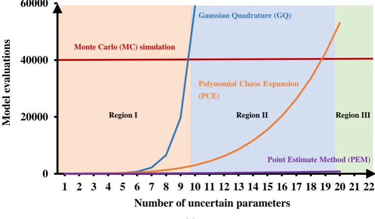
Figure 1. Computational demand (i.e., number of model evaluations) for different methods for uncertainty quantification with the increasing number of uncertainty parameters.

Various UQ methods for RO can be found in the literature. For instance, [13] used traditional sampling-based methods, i.e., (quasi) Monte Carlo (MC) simulation. Spectral methods, e.g., polynomial chaos expansion [14,15], have also been extensively used for RO [16–18], because of their adjustable complexity. Moreover, the desired statistical information can be directly calculated at low computational costs. Gaussian quadrature (GQ), which was developed for solving numerical 45

integration [19], is also a common approach for RO. These methods all have specific merits but fall short in an essential aspect: They all suffer from the deficiency of computational expense. In this work, we propose the point estimate method (PEM) [2] for probability-based RO, because the PEM has superior efficiency compared to other UQ methods as illustrated in Fig.1and provides workable accuracy against various cubature methods as concluded by [20] and [21].

50

include dependent parameters properly. The effect of parameter dependencies on the RO result is investigated and critically compared with the reference case where parameter dependencies are neglected.

This paper also provides a holistic framework for probability-based RO with the PEM. The objective function is robustified by using its first and second statistical moments. The multi-objective 60

optimization problem is transferred to a single-objective optimization problem by taking the weighted sum of these moments [5]. Moreover, we distinguish between hard and softconstraints where only the latter case needs to be robustified. Softequality constraints might also be relevant in the design of (bio)chemical processes but were rarely considered in previous RO studies [29,30]. In this work, we provide a robust formulation for soft inequality and equality constraints and 65

investigate their effects on the objective function. With the moments estimated by the PEM, the second- and fourth-moment methods introduced by [31] for structural reliability analysis are implemented to approximate the robustifiedsoftconstraints. The fourth-moment method has a more rigorous structure than the second-moment method but requires knowledge about the third and fourth statistical moments which might be challenging for the PEM as the performance degrades 70

for higher-order statistical moments. Therefore, we demonstrate and compare the performance of the two methods for approximating the robustsoftinequality constraints. Additionally, the global sensitivity analysis technique [32] is utilized to obtain a better understanding of the processes and provide information for simplifying and constructing the robust optimization problem systematically. The structure of the paper is organized as follows. Section 2 refers to the basics of 75

probability-based RO. The PEM and its extension to arbitrary and correlated parameters are described in Section 3. Section 4 provides details about robust inequality and equality constraints and approximation methods. The final structure of probability-based RO is given in Section 5. The basics of the global sensitivity analysis are given in Section6. To demonstrate the performance of the proposed RO framework, two case studies are thoroughly discussed in Section7: including a 80

classic jacket tubular reactor and a fed-batch bioreactor for penicillin fermentation. Conclusions can be found in Section8.

2. Background of probability-based robust optimization

This section starts with the problem formulation used throughout the paper and introduces the general structure of probability-based RO. First-principle models are used to describe the physical 85

and chemical effects of (bio)chemical processes mathematically. In the field of process system engineering, the models typically consist of nonlinear different algebraic equations (DAEs) equal to:

˙xd(t) =gd(x(t),u(t),p), xd(0) =x0, (1)

0 =ga(x(t),u(t),p), (2)

wheret ∈ [0,tf]denotes the time,u ∈ Rnu the control input vector, andp ∈Rnp the time-invariant parameter vector. x = [xd,xa] ∈ Rnx is the state vector while xd ∈ Rnxd and xa ∈ Rnxa are the differential and algebra states, respectively. x0 is the vector of the initial conditions for 90

the differential states. Furthermore, two types of functions gd : R(nxd+nxa)×nu×np → Rnxd and ga : R(nxd+nxa)×nu×np → Rnxa are given, which denote the differential vector field and algebraic expressions of the model.

Typically, the time-invariant parameters p and initial conditions x0 are not known exactly. Measurement and process noise give rise to uncertainties in model parameters which are estimated 95

θ= [p(ω),x0(ω)] is the vector of random variables which are functions ofω∈Ωon the probability

100

space and associated with continuous PDFsf(θ) = [f1(θ1), . . . ,fnθ(θnθ)]and correlation matrixΣ.

Parameter and initial condition uncertainties result in model-based prediction variations, i.e., the outcome of Eqs.(1) and (2) must be considered as random variables, too. Therefore, nominal (i.e., ignoring given parameter variations) optimal control problems do not give reliable solutions for realistic processes as a single realization of the uncertain parameters is used [11]. To derive reliable 105

solutions for almost all realizations of uncertain parameters, the following RO problem has to be solved.

Problem 1. Probability-based robust optimization problem

min

x(·),u(·) E[M(xtf)] +αVar[M(xtf)], (3a)

subject to:

˙xd(t) =gd(x(t),u(t),p), (3b)

0=ga(x(t),u(t),p), (3c)

xd(0) =x0, (3d)

Pr[hnq(x(t),u(t),p)≥0]≤εnq, (3e) Pr[heq(x(t),u(t),p)6=0]≤εeq, (3f)

umin ≤u≤umax. (3g)

Here,E[·]andVar[·]denote the mean and the variance of the cost functionM(xt_f), respectively, Pr[·] denotes the probability measure, α denotes a scalar weight factor, εnq and εeq are tolerance 110

factors, [umin,umax] are the upper and lower boundaries for the control input vector, andxt_f is the state vector at the end of the time horizontaltf. In detail, M(xtf)denotes a Mayer objective term that is

used for nominal optimal control problems. We should note that certain reformulations can be made to consider the optimal Lagrange control problems, too. The two functionshnq :R(nxd+nxa)×nu×np →

Rnnq andheq:R(nxd+nxa)×nu×np →Rneq are used to represent the inequality and equality constraints 115

which come from design restrictions, such as temperature limitations. Eqs. (3b) and (3c) are the model equations that as explained before will be considered as equality constraints as discussed in Section

4.

Problem 1 expresses the general formulation of the RO problem regarding probabilistic uncertainties. Eq. (3a) gives the robust form of the objective function M(xt_f), where E[M(xt_f)]

120

and Var[M(xt_f)]represent the expected performance and the robustness of the objective function, respectively. The trade-off between the performance and the robustness is adjusted by the weight factorα. Eqs. (3e) and (3f) give the robust form of the inequality and equality constraints, respectively.

They ensure that the probability of all constraint violations is less than or equal to a certain tolerance factor that can be adjusted according to given specifications and safety rules. However, to solve 125

Problem 1 practically, we have to address the following two aspects. First, the estimation of the probabilities of both constraint violations cannot be solved in closed form, and standard numerical methods might be computationally demanding. Thus, highly efficient approximation routines have to be applied to ensure representative results. Second, the robust equality constraints in Eq. (3f) are infeasible and render RO insolvable. These two aspects are discussed and addressed in the following 130

section.

3. Point estimate method (PEM)

presented by [36] but with different deterministic sample points and corresponding weights [34]. The 135

PEM has been successfully applied in the field of sensitivity analysis [37] and optimal experimental design [38–40] to quantify the influence of measurement imperfections on system identification. A brief introduction to the PEM is given in Section3.1. The concept of extending the PEM to problems with arbitrary and correlated parameter uncertainties is presented in Section3.2.

3.1. Basics of the point estimate method 140

The basic principle of the PEM is illustrated in Fig. 2. Here, a nonlinear functionk(·)with a two-dimensional parameter[ξ1,ξ2] and output[y1,y2] is used for demonstration. We assume that the two parameters have a bivariate standard Gaussian distributionξ ∼ N(0,I). The probability

distribution of the parameters does not have to be Gaussian and could follow a uniform, beta distribution or any other parametric distribution – if it is symmetric and independent [40]. First, nine deterministic sample points, i.e., the cross, circle, and star points in Fig.2, have been deliberately generated and used for function evaluations. Finally, the integral term is approximated by a weighted superposition of these function evaluations equal to:

Z

Iξ

k(ξ)f(ξ)dξ≈

np

∑

wik(ξs_i) (4)

whereξs_i denotes thei-th sample point;n_ξ andnpdenote the number of random inputs and sample points, which are equal to two and nine in this example;wiis a scalar weight factor; and f(ξ)is the

PDF of the uncertain parameters.

𝜉1

𝜉2

y1

y2

Nonlinear function

𝐲 = 𝐤(𝝃)

Figure 2.Illustration of the PEM for a nonlinear functiony =k(ξ)that has two random inputs and two random outputs; adapted from [36].

The deterministic sample points used in this work are generated by the first three generator functions (GF[0], GF[±ϑ], GF[±ϑ,±ϑ]) defined in [34] which leads to an overall number of np = 2d2+1 sample points, whered = nξ = nθ. The specific weight factors are used for each generator function which results in the final approximation scheme:

Z

Iξ

k(ξ)f(ξ)dξ≈

w0k(GF[0]) +w1

∑

∑

(5)

whereϑ =

√

3,w0=1+d 2_−7d

18 ,w1= 418−d,w2= 361 [37]. With these factors, Eq. (5) provides suitable approximations for the integral of functions with moderate nonlinearities [20,34]. In principle, we 145

Algorithm 1Sampling for correlated random variables

Initialization: Random variablesξ ∼ N(0,I),I ∈ Rd×d;θhave marginal CDFs [F1(θ1), . . . ,Fd(θd)] and correlation matrixΣ∈Rd×d;

1: Sample U = [ξ1,· · ·,ξN] with size of N = 2d2+1 fromξand dimensiond from Generator

functionGF[·];

2: Cholesky decomposition ofΣ=LLT, where L is a lower triangular matrix; 3: Correlate the sample,V=LU;

4: Convert the sample to the corresponding cumulative densityW= [F(V1),· · ·,F(Vd)]T; 5: Transform into sample ofθ,[θ1,· · ·,θN] = [F₁−1(W1),· · ·,F_d−1(Wd)]T.

3.2. Sampling strategy for independent/correlated random variables of arbitrary distributions

The proposed PEM is applicable only in the case of independent standard Gaussian distributions describing the parameter uncertainties. For most practical applications, however, we are confronted 150

with problems of arbitrary and correlated probability distributions. Therefore, we extend the PEM following Proposition 1.

Proposition 2. For two random variables (θ,ξ), whereξ ∼ N(0,I)andθhas an arbitrary distribution, and

the functionΦ(·) = F_θ−1(Fξ(·)), the following relation for the integral terms of the nonlinear function k(θ)

holds [20]:

Z

Iθ

k(θ)f(θ)dθ=

Z

Iξ

k(Φ(ξ))f(ξ)dξ. (6)

Based on Proposition 1, the integral expression with an arbitrary and correlation distribution is approximated as:

Z

Iθ

k(θ)f(θ)dθ≈w0k(Φ(ξ1)) +w1

2d+1

∑

k(Φ(ξi)) +w2

2d2₊₁

∑

k(Φ(ξj)), (7)

where the samples from the original PEM for ξ are transformed via Φ(·) = F_θ−1(Fξ(·)) to the

corresponding points inθwhich can be directly evaluated with functionk(·). The joint cumulative

density function (CDF)Fθ(θ)inΦ(·)is typically unknown in practical applications and derived from

marginal CDFs[F1(θ1), . . . ,Fd(θd)]and the correlation matrixΣ ∈ Rd×dfor the uncertain parameter

θ. Please note that it is actually infeasible to derive an analytical expression forFθ(θ)andΦ(·)[20].

Thus, we introduce Algorithm 1 adapted from [41] to transform the samples fromξtoθnumerically.

The transformed sample points can be directly used for the approximation scheme:

Z

Iθ

k(θ)f(θ)dθ≈w0k(θ1) +w1 2d+1

∑

k(θi) +w2 2d2+1

∑

k(θj). (8)

4. Moment method for approximating robust inequality and equality constraints

In this section, we discuss the details of inequality and equality constraints. In Section4.1, we categorize the constraints into two special types and discuss the effects of parameter uncertainties on 155

the constraints. In Section4.2and Section4.3, robust formulation ofsoftinequality andsoftequality constraints and methods for approximating the robustified expressions are presented.

4.1. Categorization of the constraints

optimized results satisfy physical laws. For instance, in Problem 1, equality constraints Eqs. (3b) and (3c), i.e., the governing equations, arehardconstraints as they describe the underlying (bio)chemical processes and have to be satisfied consistently. Softconstraints, in turn, do not have to be exactly satisfied under uncertainties. Softconstraints (e.g., Eqs. (3e) and (3f)) are typically imposed by the designer to restrict the design space and to satisfy additional design specifications. Therefore, soft 165

constraints can be satisfied only in a probabilistic manner and might occasionally be violated, i.e., an acceptable violation probability has to be defined for RO. Please note that the performance of the objective function may decrease if a very low violation probability is implemented. Softconstraints are considerably affected by parameter uncertainties and are investigated in the following section.

4.2. Robust formulation of soft inequality constraints 170

Soft inequality constraints do not have to be strictly satisfied but in a probabilistic manner. Inequality constraints hnq(x(t),u(t),p) ≤ 0 formulated on the probability space are also named chance constraints [43] and read as:

Pr[hnq(x(t),u(t),p)≤0]≥1−εnq, (9) where the probability of constraint satisfaction must be higher or equal to 1−εnq. Please note that Eq. (9) can also be equivalently transformed into Eq. (10) when the probability of a constraint violation is used:

Pr[hnq(x(t),u(t),p)≥0]≤εnq. (10) The probability of constraint violations is frequently estimated by MC simulations. A large number of samples are drawn from given parameter distributions, and the samples where the constraints are violated are counted. MC simulations are straightforward in implementation but require a considerable number of CPU-intensive model evaluations. The computational burden might be prohibitive, especially for the iterative nature of the RO. Moment-based approximation 175

of failure probabilities has been widely applied in the field of reliability analysis [31], and thus, this method is used as an alternative concept to approximate the chance constraints in this work. In addition, it takes the advantage of the proposed PEM for estimating the needed statistical moments.

The basic idea of the moment-based approximation method is to transform the probability distribution of the constraint functions into some existing distributions, e.g., the frequently used standard normal distribution ξ ∼ N(0, 1), and to obtain the failure probability based on the

probability. Here, the one-dimensional constraint function−hnq(x(t),u(t),p) with a negative sign is abbreviated ashnqand used in the following. The isoprobabilistic transform given in Proposition 1 is applied to express the relation between the standard normal distribution and one random variable with existing distribution as:

ξ=F_ξ−1(F_h

nq(hnq)), (11)

whereF_ξ−1indicates the inverse CDF of the standard normal distribution, andF_h

nqindicates the CDF

ofhnq. Based on this transformation, the failure probability of the constraint functionhnqis equivalent to the probability ofξ ≤ F_ξ−1(F_h

nq(0))as shown in Eq. (12). As the CDF ofξis known analytically,

the failure probability of the constraint function can be determined ifF_ξ−1(F_hnq(0))is given. However, the transformation functionF_ξ−1(F_hnq(·))is typically not available as the CDF ofhnq is unknown in practice. Thus, we aim at transformation rules that are based only on the statistical moments of hnq[31]:

Pr[hnq(x(t),u(t),p)≥0] =Pr[hnq ≤0],

=Pr[ξ≤F_ξ−1(F_h

nq(0))].

Two representative moment-based approximation methods [31], i.e., the second-moment method and the fourth-moment method, are used to estimate the failure probability with the first four statistical moments of the probability distribution of the constraint function hnq, which are named the mean (µ_h

nq), variance (σ

2

hnq), skewness (αhnq,3), and kurtosis (αhnq,4). The second-moment

method approximates the transformation function with the first two moments as in Eq. (13), while the fourth-moment method utilizes all four moments and has a more complex structure; see Eq. (14) [31]. The approximations are incorporated in Eq. (12) to calculate the failure probability of the constraints:

F_ξ−1(F_hnq(0)) =−µhnq

σ_h

nq

, (13)

F_ξ−1(F_h

nq(0)) =−

3(α_h

nq,4−1)( µ_hnq

σ_hnq) +αhnq,3(( µ_hnq

σ_hnq)

2₋₁₎

q

(9α_hnq,4−5α2_h

nq,3−9)(αhnq,4−1)

. (14)

The accuracy of the moment-based approximation methods is determined by two factors. The first factor is the intrinsic approximation error which results from the approximated transformation 180

function (Eq. (11)) using a limited number of statistical moments. By definition, the fourth-moment method has a lower intrinsic approximation error because this method is more rigorously defined with higher-order statistical moments. The second factor is the estimation error of the statistical moments, especially the higher-order moments, e.g., skewness and kurtosis. The PEM introduced in Section3is used to calculate the needed statistical moments with considerably lower computational 185

costs in comparison to MC simulations. However, the precision of the estimated statistical moments deteriorates with higher-order statistical moments, because the PEM might fail for highly nonlinear problems of higher-order terms. Thus, especially the fourth-moment method may suffer from the estimation error. According to these two sources of approximation errors, it is difficult to determine which approximation method, i.e., the second- or fourth-moment method, is superior for robust 190

process design. Therefore, we further analyze both concepts and investigate their benefits for efficient and credible robustification strategies in the following section.

4.3. Robust formulation of soft equality constraints

Similar to the inequality constraints,softequality constraints are considered in a probabilistic manner for the RO problem and are given as:

Pr[heq(x(t),u(t),p)6=0]≤εeq (15) However, Eq. (15) is not directly solvable for most applications as the constraint functionheqhas a continuous probability distribution. In other words, the probability of a single point is equal to zero when the random space is continuous [44]. Thus, we can find that:

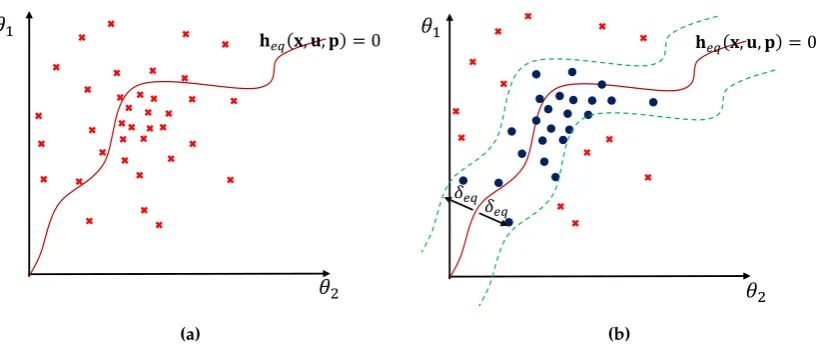
Pr[heq(x(t),u(t),p)6=0] =1, (16) which contradicts Eq. (15) ifεeq 1. Note that we aim to satisfy the equality constraint with high probability, and thusεeq 1. Fig. 3ashows an example of the equality constraint in the random 195

parameter space. Here, the samples are drawn from their distributions, and the curve shows the locations where the samples satisfy the constraints.

𝜃

𝜃

𝐡𝑒𝑞(𝐱, 𝐮, 𝐩) = 0

(a)

𝜃

𝜃

𝛿𝑒𝑞

𝛿𝑒𝑞

𝐡𝑒𝑞 𝐱, 𝐮, 𝐩 = 0

(b)

Figure 3. Illustration of softequality constraints heq(x,u,p) = 0. For the sake of explanation, a two-dimensional random space with uncertain parametersθ1andθ2is used. Samples satisfying the constraints are shown by blue-filled circles , while samples that violate the constraints are shown by red cross-outs . (a) The probability of samples that satisfy the equality constraint (red line ) is equal to zero for the continuous random space. (b) The equality constraint and its relaxed boundaries (green dashed line ) with widthδeq. The probability of satisfying the equality constraints is given

by the percentage of samples, i.e., , which are located within the boundaries.

admitting that samples can lie within a certain range around the constraints. Based on the relaxation, the robust equality constraints in Eq. (15) are substituted by:

Pr[−δeq≤heq(x(t),u(t),p)≤δeq]≥1−εeq, (17) whereδeqindicates the relaxation factor and determines the range of relaxed equality constraints. As we can see in Fig.3band Eq. (17), we have a region rather than a single curve where the constraint is satisfied. Thus, we can have nonzero probability, and the RO problem becomes solvable. The robust 200

equality constraints in Eq. (17) have nearly the same structure as the robust inequality constraints in Eq. (9). Therefore, the methods described in Section4.2can be used to solve Eq. (17) in RO problems immediately.

As mentioned previously, there is a trade-off between the performance of the objective function and the satisfaction probability of soft inequality and soft equality constraints. And the relevant 205

factors,εnq,εeq andδeq, have to be adapted properly. More details about how to select these factors are presented with the given case studies in Section7.

5. Robust optimization with the PEM

The final structure of the solution to the RO problem defined in Problem 1 is summarized in Eq. (18). Note thatF(·)in Eqs. (18h) and (18i) indicates the CDF of a standard Gaussian distribution. 210

The PEM is used to estimate the relevant statistical moments to include the effect of parameter uncertainties. Eqs. (18c) to (18g) are the evaluations of the dynamic system and the constraint functions for all deterministic sample points that are generated from the probability distributions of the uncertain model parameter. Based on the evaluations, Eqs. (19a) to (19f) calculate the statistical moments of the objective function and constraints which are used in Eqs. (18a), (18h), and (18i). 215

min

x(·),u(·) E[M(xtf)] +αVar[M(xtf)], (18a)

subject to:

i=1, . . . , 2d2+1, m=1, 2, 3 (18b)

θi= [pi,x0,i]T,xi= [xd,i,xa,i]T,xd,i(0) =x0,i,xtf,i =xi(tf inal), (18c) ˙xd,i(t) =gd(xi(t),u(t),pi), 0=ga(xi(t),u(t),pi), (18d)

h1,i=−hnq(xi(t),u(t),pi) (18e)

h2,i=heq(xi(t),u(t),pi) +δeq (18f) h3,i=−heq(xi(t),u(t),pi) +δeq (18g)

F(−

3(α_h

1,4−1)( µ_h

1 σ_h

1

) +α_h

1,3(( µ_h

1 σ_h

1

)2₋₁₎

q

(9α_h

1,4−5α 2

h1,3−9)(αh1,4−1)

)≤εnq (18h)

F(−

3(α_h

2,4−1)( µ_h

2 σ_h

2

) +α_h

2,3(( µ_h

2 σ_h

2

)2−1)

q

(9α_h

2,4−5α 2

h2,3−9)(αh2,4−1)

) +F(−

3(α_h

4,4−1)( µ_h

4 σ_h

4

) +α_h

4,3(( µ_h

4 σ_h

4

)2−1)

q

(9α_h

4,4−5α 2

h4,3−9)(αh4,4−1)

)≤εeq (18i)

umin≤u≤umax, (18j)

E[M(xt_f)] =w0M(xtf,1) +w1

2d+1

∑

M(xt_f,i) +w2 2d2+1

∑

M(xt_f,j), (19a)

Var[M(xt_f)] =w0(M(xtf,1)−E[M(xtf)])

2_+w

1 2d+1

∑

(M(xtf,i)−E[M(xtf)])

2

+w2 2d2₊₁

∑

(M(xtf,j)−E[M(xtf)])

2_,

(19b)

µ_hm =w0hm,1+w1

2d+1

∑

hm,i+w2 2d2₊₁

∑

hm,j, (19c)

σ_h2

m =w0(hm,1−µhm)

2_+w12d

_∑

(hm,i−µ_h

m)

2₊

w2 2d2₊₁

∑

(hm,j−µ_h

m)

2_,

(19d)

α_hm,3=

w0(hm,1−µ_h

m)

3_+w12d_∑+1 i=2

(hm,i−µ_h

m)

3_+w2 2d

2₊₁ ∑ j=2d+2

(hm,j−µ_h

m) 3 σ3 hm , (19e) α_h

m,4=

w0(hm,1−µ_h

m)

4_+w

1 2d+1

∑ i=2

(hm,i−µ_h

m)

4_+w

2 2d2₊₁

∑ j=2d+2

(hm,j−µ_h

nq)

4

σ_h4

m

, (19f)

6. Global sensitivity analysis

Before we apply the robust optimization framework, we briefly introduce the idea of global sensitivity analysis (GSA). In general, GSA is not mandatory for the robust optimization framework 220

but provides useful information for analyzing and optimizing complex systems.

GSA is a valuable tool for determining the impact of each parameter and parameter combinations on the result of a mathematical model for given parameter variations [40,46–50]. Thus, GSA determines the most relevant parameters and parameter uncertainties to be considered in RO, respectively. By focusing on the relevant parameters and neglecting the irrelevant parameter, we can 225

reduce the complexity of the RO problem considerably.

As most model parameters, which are identified via experimental data, are correlated, the effect of parameter correlation has to be considered in GSA. In this work, we present GSA methods that are capable of problems with independent parameters and problems with dependent parameters. Although parameter dependence is quite common in industrial applications, studies of GSA with 230

dependent parameters have been considered only recently; see [24–26]. Moreover, the GSA concepts can be categorized into two types: variance-based methods [32,51,52] and moment-independent methods [53]. For details about the definitions and a critical comparison of these two concepts, the interested reader is referred to [54].

Total sensitivity indices 𝑆𝑇𝑖

𝑖𝑛𝑑

First-order sensitivity indices 𝑆𝑖𝑖𝑛𝑑

Interaction sensitivity indices 𝑆𝑖,𝑗,𝑘,….𝑖𝑛𝑑

Structural total sensitivity indices 𝑆𝑇𝑖

𝑈

Structural first-order sensitivity indices 𝑆𝑖𝑈

Correlative total sensitivity indices 𝑆𝑇𝑖

𝐶

Total covariance-based total sensitivity indices

𝑆𝑇𝑖𝑐𝑜𝑣

Structural interaction sensitivity indices 𝑆𝑖,𝑗,𝑘,….𝑈

Correlative first-order sensitivity indices 𝑆𝑖𝐶

Correlative interaction sensitivity indices 𝑆𝑖,𝑗,𝑘,….𝐶 Variance-based

Sensitivity measure (Indepdendent)

Covariance-based Sensitivity measure

(Correlated)

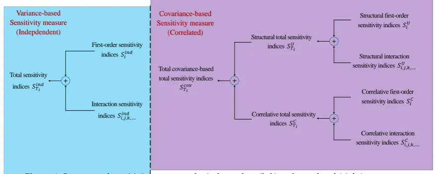
Figure 4.Structure of sensitivity measures for independent (left) and correlated (right) parameters.

Although the moment-independent method has a more rigorous definition than the 235

variance-based method, the variance-based approach is the standard in GSA and therefore, is implemented in this work. The structure and types of sensitivity indices used in the variance-based method are illustrated in Fig. 4. On the left of Fig. 4, the variance-based method defines three types of sensitivity indices for independent parameters. First-order sensitivity indicesSind_i measure the main effect of an individual parameter i on the model output, interaction sensitivity indices 240

S_iind_,j,k,...measure the dependence of the effect for two or more parameters, and total sensitivity indices Sind_Ti are the sum of the main and interactive effects of parameter i. On the right of Fig. 4, new sensitivity indices are derived from the covariance decomposition of the model output for correlated parameters. Obviously, they have the same types of sensitivity indices as the independent case but for three different groups: structural sensitivity indices SU, correlative sensitivity indices SC, and 245

total covariance-based sensitivity indicesScov. Structural sensitivity indices reflect the impact of an individual model parameter or parameter interactions on the model output and are determined by the model structure. They have the same trend as independent sensitivity indices but with different magnitudes. The correlative sensitivity indices exclusively show the impact of parameter correlations. The sum of these indices leads to total covariance-based sensitivity indices Scov that express the 250

overall impact of the correlated parameters. In this work, the first-order sensitivity indicesSind_i for the independent case and the total covariance-based first-order sensitivity indicesScov

case are sufficient, because there are few interactions between the uncertain parameters. Values of the sensitivity indices were utilized as indicators for reducing the complexity of our RO problem as demonstrated in the design of the penicillin fermentation process.

255

7. Case studies

In this section, we demonstrate the performance of the proposed framework with two case studies. In case study 1, we design an optimal jacket temperature profile for a tubular reactor considering two uncertain and correlated model parameters. Additionally, a robust equality constraint for the product temperature at the reactor outlet is assumed to incorporate process 260

intensification aspects in the design problem. In case study 2, a penicillin fermentation process is analyzed as it is of interest in the pharmaceutical industry. A fed-batch bioreactor model is used to design an optimal feeding profile under parameter uncertainties. GSA is applied to determine the influence of parameter uncertainties on the process states and to offer a more tractable problem, i.e., a reduced number of uncertain model parameters which have to be considered in the robust process 265

design.

GSA and the RO problem were solved in MATLABR_{. Parameter sensitivities for the} independent case were calculated with UQLAB [55]. The RO problem for the first case study was solved by the MATLAB function fmincon, while the RO problem for the second case study, which is more complex, was solved by the simultaneous approach [56] and implemented in the symbolic 270

framework CasADi for numeric optimization [57] using the NLP solver IPOPT [58] and the MA57 linear solver [59].

7.1. Case study 1: a jacket tubular reactor

Design of the essential part of the production process, i.e., a tubular reactor, where an irreversible first-order reaction Eq. (20) takes place, is considered as the first benchmark case study.

A−→B+C. (20)

The reactor, which is operated under the steady-state condition, is described by the following governing equations [30]:

dx1 dz =

α_kin

v (1−x1)e

γx₂

1+x_{2, (21)}

dx2 dz =

αkinδ

v (1−x1)e

γx₂

1+x_{2 +}β

v(u−x2)., (22)

wherezis the relative reactor position, 0≤z≤1. The statesx1andx2are the dimensionless forms of the reactant concentration ofAand the reactor temperature, respectively. The jacket temperature 275

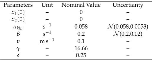
is the control input given in its dimensionless formu = (Tj−Tin)/Tin and is adjusted to meet the desired performance and robustness requirements. The control input is discretized into 25 equidistant elements constrained by 280 K and 400 K. The kinetic coefficientαkinand the heat transfer coefficient

β are assumed to be uncertain, i.e., they follow a Gaussian distribution with a standard deviation

of 10 % of their nominal values. The implemented parameter values and operating conditions are 280

summarized in Table1. For additional details of the proposed reactor model, the interested reader is referred to [30]. The conversion of the reactorCf, as well as the reactor temperature Tr, can be calculated from their dimensionless form via:

Cf(z=1) = x1(z=1), (23)

Table 1.Parameters for the tubular reactor model

Parameters Unit Nominal Value Uncertainty

x1(0) – 0 –

x2(0) – 0 –

αkin s−1 0.058 N(0.058,0.0058)

β s−1 0.2 N(0.2,0.02)

v m s−1 0.1 –

γ – 16.66 –

δ – 0.25 –

This case study aims to maximize the final conversion of reactant A while fulfilling the given 285

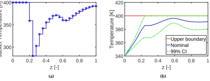
constraints on the reactor temperature. In particular, an upper boundary is added to the reactor temperature to prevent undesired side reactions. The results of the deterministic optimal design are depicted on the left of Fig. 5. As we can see, the reactor temperature increases rapidly to the upper boundary to ensure the maximum reaction rate and a final conversion of 0.996, respectively. However, numerous violations of the temperature boundary occur when the parameter uncertainties are taken 290

into account. In contrast to the deterministic process design, a robust optimal design that includes parameter uncertainties is conducted next. The corresponding results are given on the right of Fig.

5. Here, a weight factorα= 3 and a tolerance valueεnq = 1% are used for the robust objective and inequality constraints. The robust inequality constraints are approximated with the second-moment method as in Eq. (13). As we can see from the results, the temperature boundary can be satisfied with 295

a probability of 99%, at the cost of the reactor performance; i.e., final conversion decreases to 0.985.

7.1.1. Robust design with parameter correlation

Next, we investigate the influence of parameter correlation on the robust process design. We assign the two uncertain parameters αkin and β the marginal distribution shown in Table 1 and

the additional Pearson correlation coefficient of 0.8. Deterministic sample points for the correlated 300

parameters are generated with Algorithm1of the modified PEM. The structure of the RO problem is similar to that for independent parameters with a weight factorα=3 and a tolerance valueεnq=1%. Here, too, the second-moment method is applied. In Fig. 6, results for the optimal design with parameter correlations are given. As we can see, the profile of the jacket temperature has considerable differences compared to the nominal case; see Fig. 5. Especially, the drop in the jacket temperature 305

between positionz=0.5 andz=0.8 results from the parameter correlation effect. 7.1.2. Performance of the fourth-moment method

Thus far, only the second-moment method is used to approximate the robust inequality constraints. The resulting confidence intervals of the reactor temperature are illustrated with green dashed curves in Fig. 5d and 6b. We can observe that the upper boundary of the confidence 310

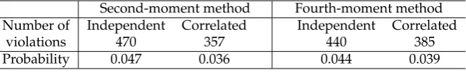
intervals are consistent with the upper limit of the reactor temperature once they approach it. However, the confidence intervals are approximated by taking into account only the first and second statistical moments and are not precise if the probability distribution of the reactor temperature is non-Gaussian. Reference values based on MC simulations with 10000 sample points are summarized in Table2. In the case of the second-moment method, the violation probabilities are 4.7% and 3.6%, 315

respectively, which exceeds the tolerance valueεnq = 1% slightly. The reason for this mismatch is mainly due to the approximation error of the robust inequality constraints while considering only the first two statistical moments.

As discussed in Section4.2, the fourth-moment method uses more statistical information than the second-moment method and has lower approximation error. The same RO problem is solved 320

0 0.2 0.4 0.6 0.8 1 z [-]

300 350 400

Jacket Temperature [K]

(a)

0 0.2 0.4 0.6 0.8 1

z [-] 300

350 400

Jacket Temperature [K]

(b)

0 0.2 0.4 0.6 0.8 1

z [-] 340

360 380 400 420

Temperature [K]

Upper boundary Nominal 99% CI

(c)

0 0.2 0.4 0.6 0.8 1

z [-] 340

360 380 400 420

Temperature [K]

Upper boundary Nominal 99% CI

(d)

Figure 5. Results for nominal design (left) and robust design (right). (a) and (b) are the optimal profiles of the jacket temperature. (c) and (d) are the evolution of the reactor temperature and the 99% confidence interval (CI). The mean and standard deviation of the conversion of reactant A have value of [0.996, 0.004] and [0.985, 0.010] for the nominal and robust design, respectively.

0 0.2 0.4 0.6 0.8 1

z [-] 300

350 400

Jacket Temperature [K]

(a)

0 0.2 0.4 0.6 0.8 1

z [-] 340

360 380 400 420

Temperature [K]

Upper boundary Nominal 99% CI

(b)

Table 2.The number of constraint violations from 10000 Monte Carlo simulations, where the robust inequality constraints are approximated by the second- and fourth-moment methods for both designs with independent and correlated parameters.

Second-moment method Fourth-moment method Number of Independent Correlated Independent Correlated

violations 470 357 440 385

Probability 0.047 0.036 0.044 0.039

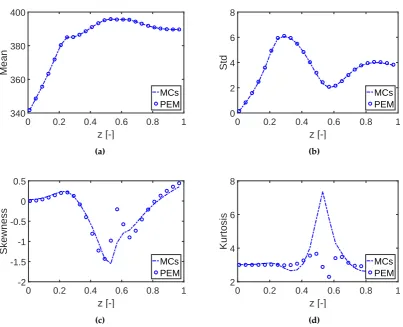
the right of Table2. However, the expected improvement could not be validated. In fact, the violation probability for the correlated case increases after the fourth-moment method is applied. The reason for this unexpected performance is mainly due to the estimation error of higher-order statistical moments. When we compare the first four statistical moments estimated by the PEM and the MC 325

simulations, we can see in Fig.7that the PEM provides useful approximations for the first and second moments and deteriorates considerably for the higher-order moments. The comparison indicates that the fourth-moment method might not be suitable for the PEM-based robust optimization framework, especially for industrial applications where the systems might be strongly nonlinear and complex. Please note that for calculating the n-th statistical moment, not only the function k(ξ) but also

330

k(ξ)n has to be approximated which is challenging for all sample-based approximation schemes,

including MC simulations [2]. The fourth-moment approach, in turn, is still a promising way to approximate probability distributions if the higher-order moments can be estimated accurately, e.g., using polynomial chaos expansion or Gaussian mixture density approximation [60]. Based on this finding, in the following section, we exclusively implement the second-moment method when we 335

use the PEM.

Alternatively, one might adjust the tolerance value for the robust inequality constraints to mitigate the effect of approximation errors when using the second-moment method. The violation probabilities of the inequality constraints for the robust design with different tolerance values are given in Fig. 8. As we can see, the probability can achieve 0.01 by setting the tolerance value to 340

0.002 for the independent and correlated cases. Fortunately, the average conversion of reactantAwas significantly impacted by changing the tolerance value; see Fig.8.

7.1.3. Impact of robust equality constraints

Here, we would like to investigate the effect of robust equality constraints that might result from design specifications. The design of continuous processes follows the trend of process integration and intensification to reduce energy costs and raw material. For instance, to avoid extra cooling expenses for a downstream process, we integrate the heat management into the reactor design directly. To this end, a terminal equality constraint is added to lower the outlet temperature to the value of the inlet temperature:

|Tr(z=1)−Tr(z=0)|=0. (25)

With this additional soft equality constraint, there exists a trade-off between maximizing the reactant conversion while minimizing the temperature difference. First, the results of the reactor design where 345

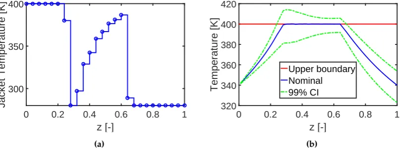
we neglect parameter uncertainties are given in Fig. 9a. The jacket temperature drops sharply to its lower limit for the second half of the reactor, and the outlet temperature returns exactly to 340 K. Consequently, the reactant conversion decreases almost 2% compared to the nominal design without the equality constraint (Fig. 5). Next, the effect of parameter uncertainties on the nominal design is illustrated in Fig. 9bwith the green dotted line. Because of limited space, we mainly consider 350

0 0.2 0.4 0.6 0.8 1 z [-]

340 360 380 400

Mean

MCs PEM

(a)

0 0.2 0.4 0.6 0.8 1

z [-] 0

2 4 6 8

Std

MCs PEM

(b)

0 0.2 0.4 0.6 0.8 1

z [-] -2

-1.5 -1 -0.5 0 0.5

Skewness

MCs PEM

(c)

0 0.2 0.4 0.6 0.8 1

z [-] 2

4 6 8

Kurtosis

MCs PEM

(d)

Figure 7.A comparison of the first four statistical moments estimated with the point estimate method (PEM) and Monte Carlo (MC) simulations for the reactor temperature in case study 1. Std is the abbreviation of standard deviation.

0.002

0.005

0.01

Tolerance value

"

[-]

0.01

0.02

0.03

0.04

0.05

Probability of violation [-]

0.98

0.982

0.984

0.986

0.988

Average conversion [-]

Ind (Pro)

Cor (Pro)

Ind (Con)

Cor (Con)

relaxation factorsδeq and tolerance factorsεeq are used to demonstrate the effect of robust equality 355

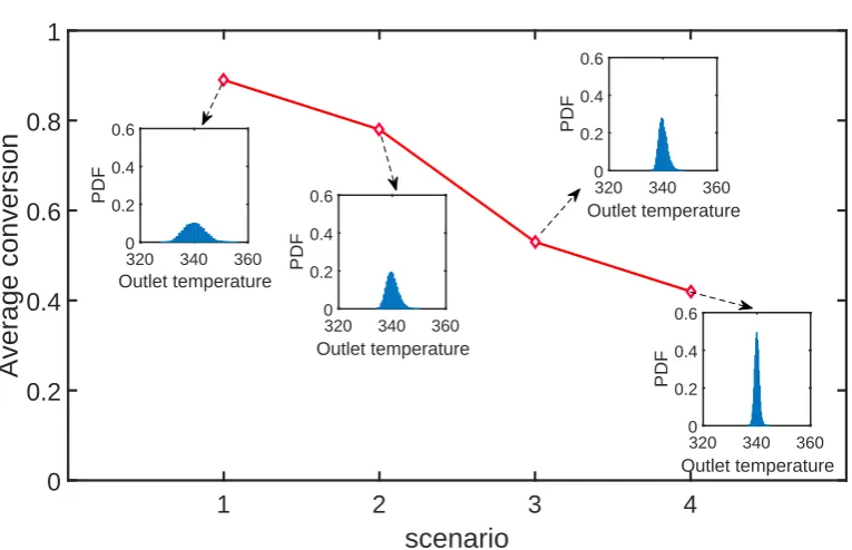
constraints on the process performance. Values for the relaxation factors and results are summarized in Fig. 10. We can see that the probability distribution of the outlet temperature narrows quickly once we reduce the relaxed region and violation probability while the performance of the reactor (the reactant conversion) deteriorates considerably. The process engineer has to decide on the trade-off between product performance and energy expense. Note that the robust inequality constraints in 360

these scenarios are always satisfied and thus, are not explicitly shown here.

0 0.2 0.4 0.6 0.8 1

z [-] 300

350 400

Jacket Temperature [K]

(a)

0 0.2 0.4 0.6 0.8 1

z [-] 320

340 360 380 400 420

Temperature [K]

Upper boundary Nominal 99% CI

(b)

Figure 9. Results for the nominal design with terminal equality constraints. (a) optimal jacket temperature profile. (b) evolution of the reactor temperature with its 99% confidence interval (CI). The mean and standard deviation of the conversion of reactantAare 0.980 and 0.016, respectively.

7.2. Case study 2: fed-batch bioreactor for fermentation of penicillin

The performance of the PEM-based robust optimization framework is also demonstrated with a fermentation process as illustrated in Fig. 11. Fermentation processes have received great interest in the pharmaceutical industry, and in this study, we try to optimize the penicillin fermentation [61]. To this end, we design a feeding substrate profile that ensures the optimal performance and robustness of the bioreactor. A fed-batch reactor model is used based on the following assumptions: 1) ideal mixing of all components in the bioreactor, 2) isothermal condition in the reactor, and 3) the effect of the oxygen transfer can be neglected by considering an upper limitation on the biomass and substrate concentrations. The mathematical model for the fermentation process reads as:

dX

dt =µX− F

VX (26)

dS dt =−

µ

YxX − θp

YpX

−mxX+ F

V(Sf−S) (27)

dP

dt =θpX−KP− F

VP (28)

dV

dt =F, (29)

1

2

3

4

scenario

0

0.2

0.4

0.6

0.8

1

Average conversion

320 340 360

Outlet temperature

0 0.2 0.4 0.6

PDF

320 340 360

Outlet temperature

0 0.2 0.4 0.6

PDF

320 340 360

Outlet temperature

0 0.2 0.4 0.6

PDF

320 340 360

Outlet temperature

0 0.2 0.4 0.6

PDF

Figure 10. The average conversion of reactantAand the probability density function of the outlet temperature for four scenarios that have different relaxation factorsδeqand tolerance factorsεeq. 1:

δeq=5,εeq=10%, 2:δeq=5,εeq=1%, 3:δeq=2,εeq=10%, 4:δeq=2,εeq=1%.

Medium Substrate

Mixing

Heat Sterilization

Sterile Air

Air Compressor

Air Filtration

Exhaust Air Filtration

Storage

Downstream Process: Removal Biomass, Extraction, Crystallization, Drying Optimal feeding profile

Cooling

Cooling

Table 3.Nominal values of the model parameters and the initial conditions for the fed-batch model

Parameters Unit Nominal Value Parameters Unit Nominal Value

µm 1/h 0.11 mx 1/h 0.029

Kx – 0.006 Sf g/L 400

θm 1/h 0.004 t h 0–80

Kp g/L 0.0001 X(0) g/L 1

Ki g/L 0.1 S(0) g/L 0.5

K 1/h 0.01 P(0) g/L 0

Yx – 0.47 V(0) L 250

Yp – 1.2

constant concentrationSf and a time-dependent flow rateF. The specific growth rate of the biomass

µand the productθpis represented by the substrate inhibition kinetic with the following form:

µ= µmS

S+KxX (30)

θp= θmS

S+Kp+S2/Ki

. (31)

The initial conditions of the state variables and the nominal value of the other kinetic parameters are listed in Table3. Further details about the model are given in [61].

First, the process is optimized assuming that all parameters are estimated precisely; i.e., 365

parameter uncertainties are neglected. The goal is to maximize the final concentration of product P on a fixed time range while the concentration of biomass Xand substrateSshould be below 40 g/L (limited by the oxygen transfer capacity) and 0.5 g/L (to avoid side reactions) for the entire time horizon, respectively [62]. The control variableFis parametrized with 100 elements which are bounded within the range of [0,10]. The resulting dynamic optimization problem is solved with the 370

nominal value of all parameters, and the results are shown in Fig. 12. Here, the feed rate of the substrate is adjusted to keep the substrate concentration equal to 0.5 g/L at which the maximum growth rate of the biomass is achieved at the beginning. After the biomass concentration reaches its upper limit, the substrate concentration drops nearly to zero to cease the self-reproduction of the biomass. Moreover, the substrate is still fed with a low rate that is consumed by the biomass to 375

produce the desired product.

However, due to imperfect measurement data and because of model simplifications, the first nine model parameters are uncertain and might be correlated. Based on the results given in [63], we assign the nine parameters with a multivariate normal distribution, where their marginal distributions have mean values equal to the nominal values and standard deviations equal to 10% of the nominal values. 380

To investigate the effect of parameter correlations, two situations are analyzed: 1) The parameter correlations are neglected, and the correlation matrixΣis set to an identity matrix; 2) the correlation coefficients of µm,θm,Yx, and mx in Σ are set to 0.95. The effect of imprecise model parameters on the process performance is also shown in Fig. 12with the blue dotted lines. Strong violation of the constraints and large variation of the product quality are observed, and thus, the parameter 385

uncertainty has to be considered in the process design for robustness. Please note that the negative confidence interval (CI) of the substrate concentration stems from the assumption that the CIs are symmetric and directly derived from the mean and variance of the states.

7.2.1. Global sensitivity analysis

Before solving the RO problem for the fermentation process, we want to decrease its 390

0 20 40 60 80 t [h]

0 2 4 6

Feed rate [L/h]

(a)

0 20 40 60 80

t [h] 0

10 20 30 40 50

Biomass [g/L]

mean 99% CI limit

(b)

0 20 40 60 80

t [h] -20

-10 0 10 20 30

Substrate [g/L]

nominal 99% CI limit 0 20 40 60 80

t [h] 0 0.2 0.4 0.6

Substrate [g/L]

(c)

0 20 40 60 80

t [h] 0

2 4 6

Product [g/L]

nominal 99% CI

(d)

calculated for the biomass and substrate concentrations in addition to the product concentration at the final time point, i.e., for those quantities involved in either the objective function or the constraints of the optimization problem. Figs.13a,13c, and14ashow the sensitivity results for the independent 395

case. As we can see, the biomass and product concentrations are strongly affected by parameters

µm,θm,Yx, and mx, while the other parameters have a minor impact. Moreover, by summing up the first-order sensitivity indices, the interaction among the parameters are negligible. Next, we calculate the correlative (SC) and total covariance-based (Scov) first-order sensitivity regarding the biomass, substrate, and product concentration; see Figs. 13b,13d, and14b. Here, we do not show 400

the results for the structural sensitivity indices and all the total sensitivity indices. The reason is that the model structure does not change with the existence of parameter correlations, and thus, the structural sensitivity indices and parameter interactions are similar to those for the independent case. Nevertheless, an evident effect of parameter correlations on the sensitivity analysis result can be observed from the figures: They have a completely different trend compared to the independent 405

case. The sensitivity results from the correlated case also suggest considering the uncertainties and correlations from µm, θm,Yx, andmx for the RO problem. By using the information from the sensitivity analysis, we significantly reduce the number of required PEM points for the RO problem. The number of model evaluations for each optimization iteration decreases from 2×92+1 = 163 to 2×42+1 = 33 for the independent and correlated cases. Finally, the performance of RO with 410

parameter uncertainties of identified sensitive is studied in the following section.

7.2.2. Robust optimization

The RO is solved with the framework proposed in Section5. To this end, a weight factorα= 3

and a tolerance valueεnq=1% are used for the robust objective and inequality constraints. The PEM points for RO are generated only for the sensitive parameters identified via GSA, i.e., four parameters 415

are considered. First, the RO is solved for the simplifying assumption of the independent parameters using the same uncertainty setting of the previous case study. The evolution of the mean and 99% CIs for the biomass and the substrate are illustrated in Fig. 15. The biomass accumulates rapidly until its CI approaches the upper boundary to maximize the productivity while the CI of the substrate remains at its upper boundary at the beginning and decreases to a low value to activate the production 420

phase. However, the result of the RO while ignoring parameter dependencies is too conservative. The effect of parameter dependencies is shown in Fig. 16 for the previous optimized setting, i.e., assuming independent parameters. The shape of the CIs of the biomass and the substrate are quite different from those in Fig. 15 and do not reach their upper boundaries which leave some space for improvement. Therefore, we repeat the RO considering the parameter dependencies accordingly 425

and plot the results in Fig. 17. As we can see, the CIs of both biomass and substrate concentration reach the upper boundaries and are less conservative compare to the results in Fig.16.The optimized feeding profile of the substrate for the independent and correlated cases are compared in Fig. 18a. The substrate for the correlated case is fed with a higher rate and descended a bit earlier than that for the independent scenario. The PDFs of the product concentrations at the final time point shown 430

in Figs. 16and17are compared in more detail in Fig. 18b. The product concentration is improved considerably as the dashed curve, which represents the parameter dependency case, is a bit narrowed and shifted to higher concentration.

As mentioned, the negative CIs of the substrate concentration in all the figures are due to the assumption of symmetric distributions of the states. This also indicates that the CIs might not be 435

accurate, and thus, we validate them by checking the number of constraint violations from 10000 Monte Carlo simulation for the independent and correlated cases, where the corresponding optimal feeding profiles are applied. The results are listed in Table4. As we can see from the second row, the violation frequencies are higher than our expectation,εnq =1% = ₁₀₀₀₀100 , especially for the substrate concentration. Although the violation frequencies might be acceptable for industrial applications, we 440

0 20 40 60 80 t [h] 0 0.5 1 Sensitivity [-] u_m K_x 3_m K_p K_i K Y_x Y_p m_x (a)

0 20 40 60 80

t [h] 0 0.5 1 Sensitivity [-] u_m K_x 3_m K_p K_i K Y_x Y_p m_x (b)

0 20 40 60 80

t [h] -1 0 1 2 3 Sensitivity [-] u_m K_x 3_m K_p K_i K Y_x Y_p m_x (c)

0 20 40 60 80

t [h] -1 0 1 2 3 Sensitivity [-] u_m K_x 3_m K_p K_i K Y_x Y_p m_x (d)

Figure 13. Sensitivity results of the nine parameters on the biomass and substrate concentrations for the independent case (a) first-order sensitivity indices for the concentration of biomass X, (b) first-order sensitivity indices for the concentration of substrate S, and correlated case (c) total covariance-based first-order sensitivity indices for biomass X, (d) total covariance-based first-order sensitivity indices for substrate S.

u

m Kx 3m Kp Ki K Yx Yp mx

0 0.2 0.4 0.6 0.8 1 Sensitivity [-] First-order Total (a) u

m Kx 3m Kp Ki K Yx Yp mx

-0.5 0 0.5 1 Sensitivity [-] SC Scov (b)

results are shown in the third row of Table4. All violation numbers are improved, while we slightly lower the reactor performance regarding the penicillin productivity. Please note that the violation numbers can be further improved by also adapting the tolerance factor.

0 20 40 60 80

t [h] 0

10 20 30 40

Biomass [g/L]

mean 99% CI limit

(a)

0 20 40 60 80

t [h] -0.2

0 0.2 0.4 0.6

Substrate [g/L]

mean 99% CI limit

(b)

Figure 15. Evolution of the mean and 99% confidence interval (CI) of the biomass and substrate concentrations for the robust design of the fed-batch bioreactor, where the uncertain parameters are independent. The feeding profile from the robust design with independent uncertain parameters is applied.

0 20 40 60 80

t [h] 0

10 20 30 40

Biomass [g/L]

mean 99% CI limit

(a)

0 20 40 60 80

t [h] -0.2

0 0.2 0.4 0.6

Substrate [g/L]

mean 99% CI limit

(b)

Figure 16. Evolution of the mean and 99% confidence interval (CI) of the biomass and substrate concentrations for the robust design of the fed-batch bioreactor, where the uncertain parameters are correlated. The feeding profile from the robust design with independent uncertain parameters is applied.

8. Conclusions 445

Uncertainties in (bio)chemical processes pose difficulties in process design and necessitate the development of robust optimization strategies. Most robustification concepts, however, are limited by either their computational expense or their approximation accuracy. Moreover, standard robustification strategies do not cover the implementation of processes withsoftequality constraints and parameter dependencies which are quite common in practical applications. In this work, we 450

0 20 40 60 80 t [h]

0 10 20 30 40

Biomass [g/L]

mean 99% CI limit

(a)

0 20 40 60 80

t [h] -0.2

0 0.2 0.4 0.6

Substrate [g/L]

mean 99% CI limit

(b)

Figure 17. Evolution of the mean and 99% confidence interval (CI) of the biomass and substrate concentrations for the robust design of the fed-batch bioreactor, where the uncertain parameters are correlated. The feeding profile from the robust design with correlated uncertain parameters is applied.

0 20 40 60 80

t [h] 0

2 4 6

Feed rate [L/h]

Ind Cor

(a)

0 2 4 6

Product [g/L] 0

0.5 1

PDF [-]

Ind Cor

(b)

Figure 18.Results for the robust design of the fed-batch bioreactor, where the uncertain parameters are either independent or correlated. (a) control sequence for substrate feeding, and (b) final concentration of the product, respectively.

Table 4.The number of constraint violations from 10000 Monte Carlo simulations, where the tolerance factorεnq=1% andεnq=0.14% for both designs with independent and correlated parameters. The

performance indicates the mean value of the production concentration at the end.

independent correlated

εnq=1% X 146 35

S 572 554

performance 3.63 3.76

εnq=0.14% X 19 2

S 378 369

approximate robust equality and inequality constraints. In addition, we used the outcome of the global sensitivity analysis in the robust design to lower the computational demand considerably. 455

Two case studies, which include chemical and biological production processes, were used to demonstrate the performance of the proposed framework. The first case study attempts to maximize the conversion of a reactant while simultaneously satisfying the constraints on the reactor temperature of a tubular reactor, which is an essential process unit in continuous production processes. The proposed method can successfully give the trade-off between performance and 460

robustness for the reactor under parameter uncertainties. We observed an evident influence of parameter correlation on the designed control profile and confidence regions of the system states. The performance of the second- and fourth-moment methods for approximating the robust inequality constraints was also examined. The fourth-moment method has a more rigorous structure compared to the second-moment approach. However, the performance of the fourth-moment method is limited 465

by the accuracy of the PEM. Thus, we concluded that the second-moment method might be more favorable in this particular case. Furthermore, the approximation error could be compensated by using more conservative tolerance values, which resulted in slight deterioration of the reactor performance. To save energy costs, we also added an equality constraint to the outlet temperature. The robust equality constraint had to be relaxed deliberately to be solvable. The process performance 470

deteriorated dramatically with lower relaxation factors. The second example is the optimal design of a bioreactor for a penicillin fermentation process. Global sensitivity analysis was used successfully to determine the relevant parameters and to ease the computational expense of the framework. This is extremely useful for large-scale problems with a high number of uncertain parameters. Moreover, the effect of parameter correlations on the results was also observed. Here, the PEM still performs 475

reasonably for this complex problem and retains a relatively low computational cost.

In conclusion, the proposed framework provides a comprehensive strategy for robust optimization problems and covers features that were not considered in previous works. However, some limitations are worth noting. The PEM might fail in estimating higher-order statistical moments, especially for systems with strong nonlinearities. This is also the main reason why 480

the performance of the fourth-moment method did not provide the expected improvement in robustification. Alternatively, the precision of the PEM could be increased, or different methods for uncertainty quantification might be studied. Future work will focus on this issue.

Acknowledgments:We acknowledge support by the Open Access Publication Funds of the TU Braunschweig. Funding of the "Promotionsprogramm µ-Props" for Xiangzhong Xie by MWK Niedersachsen is gratefully 485

acknowledged. Moreover, the anonymous reviewers deserve special thanks for their valuable input.

Bibliography

1. Biegler, L.T.Nonlinear programming: concepts, algorithms, and applications to chemical processes; SIAM, 2010. 2. Schenkendorf, R. Optimal experimental design for paramter identification and model selection. PhD

thesis, Otto-von-Guericke-Universität Magdeburg, 2014. 490

3. Mortier, S.T.F.; Van Bockstal, P.J.; Corver, J.; Nopens, I.; Gernaey, K.V.; De Beer, T. Uncertainty analysis as essential step in the establishment of the dynamic Design Space of primary drying during freeze-drying. European Journal of Pharmaceutics and Biopharmaceutics2016,103, 71–83.

4. Taguchi, G.; Clausing, D.; others. Robust quality.Harvard Business Review1990,68, 65–75.

5. Vallerio, M.; Telen, D.; Cabianca, L.; Manenti, F.; Van Impe, J.; Logist, F. Robust multi-objective dynamic 495

optimization of chemical processes using the Sigma Point method. Chemical Engineering Science2016, 140, 201–216.

6. Xie, X.; Schenkendorf, R.; Krewer, U. Robust design of chemical processes based on a one-shot sparse polynomial chaos expansion concept. Computer Aided Chemical Engineering2017,40, 613–618.

7. Nagy, Z.K.; Braatz, R.D. Worst-case and distributional robustness analysis of finite-time control 500