Comparative Analysis of General Power Flow
and Optimal Power flow using Linear
Programming Method
Gargi Roy
1,
Sujan Santra
2, and Sagar Bakshi
3Modern Institute of Engineering & Technology, West Bengal, India
ABSTRACT: In power system, power flow is very essential.Power is generated at the generating station and then it flows through transmission lines.General power flow does not need any limits of bus voltage or generator voltage or any other limits.In this paper,a practical method is used by which we can solve the the problem of power flow by using control variables. The control variables are real power, reactive power and transformer ratios with automatic adjustment to minimize instantaneous costs or losses. Minimization of the costs and losses are needed to transform a general power flow to an optimal power flow.Here linear programming method which can deal with constraints of inequality and converge easily, has been applied simulation by using matpower 4 1and matlab 2010 for solving the power flow problem and comparing it with optimal power flow solutions.
KEYWORDS: Optimal power flow, Linear Programming method, Mat power, Inequality constraints, LPOPF.
I. INTRODUCTION
Now a days Energy requirements is increasing gradually.So,Grid system is very known system to provide a huge amount of power.It is used to interconnect the generation, transmission and distribution system and can provide synchronised power. So it plays a great role now-a-days. To run the grid system economically, generation cost has to be minimum.A power flow analysis means that a steady-state analysis by which voltage, current, real power, and reactive power can be found under loaded conditions.
Power flow studies is used for planning of system operation. For example, if a transmission line is be taken off line for maintenance, can the remaining lines in the system handle the required loads without exceeding their rated values. [1] The objective of this project is to transform MATPOWER program which is used in MATLAB. Considering the hurdle occurs in solving Power flow problem due to nonlinear constraints, OPF is modeled in a linear way by linear programming method. The first person who solved an exact optimization problem with the use of linear programming taking into consideration system equality and inequality constraints was Carpentier.
The main aim goal is to minimize the generation cost in time of maintaining the security of the system.To maintain the system security all devices should be in desired operation range in steady state condition[2]
System sequirity depends on the maximum output and input of generator, mva flow of transmission line and transformer and also system bus voltages.System bus voltage should be kept within specified limit.OPF is performed under steady state condition.OPF can be determined the marginal cost data of the system.In the pricing of MW transactions,system marginal cost data plays a great role.
II. LINEAR PROGRAMMING METHOD
where for each constraint one and only one of the signs <=, =, >= holds, but the sign may vary from one constraint to another. Now we need the values of xj which satisfy equation (1) and
xj >=0, j= 1, ……, r (2)
which maximize or minimize a linear function
z = h1x1 + ….. + hrxr (3)
Here pij, qi, hj are known constants.
A programming problem is linear if, in the constraints and function to be optimized, the variables appear only as linear forms. Linear Programming is a generalized form of Linear Algebra. [3]
It can handle a variety of problems.It is a mathematical method which can do a best outcome of a mathematical model. It can perform the optimization technique of linear objective function.
This method helps to maximize or minimize a linear function which is made of a bunch of constraints which are linear in nature It consists of
a set of decision variables -The values of the variables of the problem are unknown The variables represent the things which can be controlled or adjusted.The objective is to find out the values of the variable that provide the best result of the objective function ·
an objective function - It is a mathematical expression.It combines with variable to reveal the goal.It can be maximized or minimized
a set of constraints - These are the mathematical interpretation which merge the variables to limits for getting the feasible solutions.
Variable bounds - rarely some variables in an optimization problem allowed to take any value from minus infinity to plus infinity. Instead the variables usually have bounds
III. BLOCK DIAGRAM OF THE WHOLE PROCESS
The strategy for solution of LPOPF is as follows:-
IV. RESULTS
Newton's method power flow converged in 3 iterations.
System summary
TABLE I
Elements
No. of
Elements P (MW) Q (MVAR)
buses 5 300 30.0 to 140.0
generators 3 300 30.0 to 140.0 Committed
generators 3 153.1 73.2
loads 4 150 95
Fixed 4 150 95
Dispatchable 0 0 0
Shunt 0 0 0
braches 7 3.05 9.16
transformers - 30.9
Inter-ties 0 0
areas 1
TABLE II
Parameters Minimum Maximum
Voltage Magnitude
0.990 p.u. @ bus 5 1.060 p.u. @ bus 1
Voltage Angle -4.41 deg @ bus 5 0.00 deg @ bus 1
P Losses (I^2*R) 1.30 MW @ line 2-5
Q Losses (I^2*X) 3.89 MVAR @ line 2-5
Bus Data
TABLE III
Bus # Voltage Generation Load
Mag(pu) Ang(deg) P (MW) Q
(MVAR)
P (MW) Q
(MVAR)
1 1.06 0 83.05 7.27 - -
2 1.045 -1.782 40 41.81 20 10
3 1.03 -2.664 30 24.15 20 15
4 1.019 -3.243 - - 50 30
5 0.99 -4.405 - - 60 40
Total
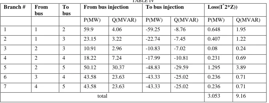
Branch Data
TABLE IV
Branch # From
bus
To bus
From bus injection To bus injection Loss(I^2*Z))
P(MW) Q(MVAR) P(MW) Q(MVAR) P(MW) Q(MVAR)
1 1 2 59.9 4.06 -59.25 -8.76 0.648 1.95
2 1 3 23.15 3.22 -22.74 -7.45 0.407 1.22
3 2 3 10.91 2.96 -10.83 -7.02 0.08 0.24
4 2 4 18.22 7.24 -17.99 -10.81 0.231 0.69
5 2 5 50.12 30.37 -48.83 -29.59 1.295 3.89
6 3 4 43.58 23.63 -43.33 -25.02 0.236 0.71
7 4 5 43.58 23.63 -43.33 -25.02 0.236 0.71
total 3.053 9.16
Result of optimal power flow Converged in 2.33 seconds
Objective Function Value = 5296.69 $/hr
System summary
TABLE V
Elements No. of
elements
P(MW) Q(MVAR)
Buses 9 820 -900.0 to 900.0
Generators 3 820 -900.0 to 900.0
Committed gens
3 318.3 -9.6
loads 3 315 115
fixed 3 315 115
dispatchable 0 -0.0 of -0.0 -0.0
shunts 0 -0.0 0.0
branches 9 3.31 36.46
transformers 0 - 161.1
Inter-ties 0 0.0 0.0
areas 1
TABLE VI
Parameters Minimum Maximum
Voltage magnitude 1.072 p.u @ bus 9 1.100 p.u. @ bus 8
Voltage angle -4.62 deg @ bus 9 4.89 deg @ bus 2
P losses - 1.39 MW @ line 8-9
Q losses - 9.36 MVAr @ line 8-2
Lambda P 24.03 $/MWh @ bus 2 25.00 $/MWh @ bus 9
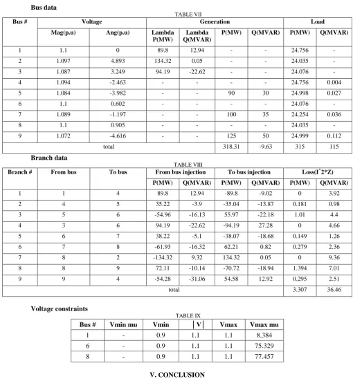
Bus data
TABLE VII
Bus # Voltage Generation Load
Mag(p.u) Ang(p.u) Lambda
P(MW)
Lambda Q(MVAR)
P(MW) Q(MVAR) P(MW) Q(MVAR)
1 1.1 0 89.8 12.94 - - 24.756 -
2 1.097 4.893 134.32 0.05 - - 24.035 -
3 1.087 3.249 94.19 -22.62 - - 24.076 -
4 1.094 -2.463 - - - - 24.756 0.004
5 1.084 -3.982 - - 90 30 24.998 0.027
6 1.1 0.602 - - - - 24.076 -
7 1.089 -1.197 - - 100 35 24.254 0.036
8 1.1 0.905 - - - - 24.035 -
9 1.072 -4.616 - - 125 50 24.999 0.112
total 318.31 -9.63 315 115
Branch data
TABLE VIII
Branch # From bus To bus From bus injection To bus injection Loss(I^2*Z)
P(MW) Q(MVAR) P(MW) Q(MVAR) P(MW) Q(MVAR)
1 1 4 89.8 12.94 -89.8 -9.02 0 3.92
2 4 5 35.22 -3.9 -35.04 -13.87 0.181 0.98
3 5 6 -54.96 -16.13 55.97 -22.18 1.01 4.4
4 3 6 94.19 -22.62 -94.19 27.28 0 4.66
5 6 7 38.22 -5.1 -38.07 -18.68 0.149 1.26
6 7 8 -61.93 -16.32 62.21 0.82 0.279 2.36
7 8 2 -134.32 9.32 134.32 0.05 0 9.36
8 8 9 72.11 -10.14 -70.72 -18.94 1.394 7.01
9 9 4 -54.28 -31.06 54.58 12.92 0.295 2.51
total 3.307 36.46
Voltage constraints
TABLE IX
Bus # Vmin mu Vmin │V│ Vmax Vmax mu
1 - 0.9 1.1 1.1 8.384 6 - 0.9 1.1 1.1 75.329 8 - 0.9 1.1 1.1 77.457
V. CONCLUSION
components of the busbar voltages. The nonlinearities have quadratic nature. By Gradient and relaxation methods, the problems can be solved.
The power flow problem is one of the basic problems.Here, load powers and generator powers both are given.On the contrary, optimal power flow problem some adjustments are made according to some specified criteria for generated power bus voltage etc.In this case, generating cost should be the minimum.It can be determined that the voltages at nodes where the loads are supplied along with the input power.Mathematics is more needed in optimal power flow problem.Here we have some limits of voltage, power beyond which we cannot let the output go because violation of those limits,fault will be occurred and the system will become damaged.
Now a more realistic definition is wanted for practical requirement, adding the statement of constraints. In reality any variable in the system will be limited because it changes the mathematical nature of the problem excessively. Whenever a variable reaches its upper or lower limit, it becomes a fixed quantity and the method of solution has to recognize it as such and be sure that the fixed quantity is optimal. [4]
The problems of ordinary power flow can be easily handled by using optimal power flow. So this method is more superior to ordinary power flow method. In this project we use linear programming method for solving any OPF problem.
REFERENCES
[1] http://www.egr.unlv.edu/~eebag/Power%20Flow%20Analysis.pdf
[2] C.L. Wadhwa, ” Electrical Power Systems”, 6th edition, pp. no.820-830, 2010
[3] http://web.williams.edu/Mathematics/sjmiller/public_html/416/currentnotes/LinearProgramming.pdf [4] http://rajanandpec.hubpages.com/hub/Optimal-power-flow-algorithm
[5] http://www.arpapress.com/volumes/vol12issue2/ijrras_12_2_20.pdf [6] ieeexplore.ieee.org