Flow-Stabilized Solids: From Colloids to Bacteria.

ABSTRACT

LINDAUER, SCOTT M. Flow-Stabilized Solids: From Colloids to Bacteria. (Under the direction of Karen E. Daniels and Robert Riehn).

Flow-stabilized solids (FSS) are a class of fragile matter that forms when a dense suspension of microscopic particles accumulates in a fluid flow against a semi-permeable barrier if the flow rate is

above a critical value. The flow rate required to form solids is known as the critical flux and can be

defined with respect to the Péclet number, which is a dimensionless ratio of advection and diffusion. The Péclet number provides a means to characterize the effect of fluid flow (advection) on both

thermal and active particles’ solid formations. However, prior work has not been able to determine

a clear thermal to athermal transition for colloidal solids, nor whether active, living matter can form flow-stabilized solids.

In this thesis, I formed microscopic solids with repulsive colloids and bacteria that are dependent

upon fluid flow. With these flow-stabilized solids (FSS), I determined that the a thermal to athermal transition occurs with respect to the Péclet number and that active, living matter can form FSS that

do not create biofilms. Flow-stabilized solids (FSS) act as a model system for crossflow and dead-end

filtration, as the barrier is a simple, one-pore membrane and the fluid flow applies both compressive (parallel) and shear (perpendicular) forces. Filter fouling is caused by solid formation on membranes,

similar to the FSS formed in our system. In Chapter’s 1 & 2, I introduce the background literature and

physics and describe the methods and instrumentation utilized throughout the thesis. In Chapter 3, I investigate the formation of FSS with mono-dispersed suspensions of hard sphere colloids at

various sizes. I will show that the critical Péclet number for solid formation is dependent on particle

size, however, a transition occurs for FSS from thermal to athermal, with respect to the fluctuations, that is not dependent upon microsphere size. These findings enable a stronger comprehension of

the mechanics of filter fouling. In Chapter 4, I form FSS with suspensions ofE. coliat different flow

velocities. I show that FSS can form with active, living matter, but do not form biofilms, which gives rise to considering microcolony formations that precede biofilm maturation. Furthermore, I show

that these solids undergo a transition in size, shape, and internal orientation based on the life cycle

phase the cells are in. In Chapter 5, I perform experiments that utilize properties of FSS. I show that FSS can be formed with shaped particles, an electric field can be applied to dissipate FSS, and DNA

© Copyright 2019 by Scott M. Lindauer

Flow-Stabilized Solids: From Colloids to Bacteria

by

Scott M. Lindauer

A dissertation submitted to the Graduate Faculty of North Carolina State University

in partial fulfillment of the requirements for the Degree of

Doctor of Philosophy

Physics

Raleigh, North Carolina

2019

APPROVED BY:

DEDICATION

BIOGRAPHY

I was born in Cary, NC on January 9, 1991. I moved to Apex, NC during middle school and attended Apex High School afterwards. My parents are both engineers who promoted the importance of

mathematical and scientific pursuits. My interest in physics stems from the AP Physics course I took

in high school, taught by Mr. Friedman. In fact, this course caused me to change my major from general engineering to physics. In May 2009, I graduated from Apex High School.

I obtained a BS in Physics from Clemson University in May 2013. During my undergraduate studies, I encountered a wide range of research topics within physics. I spent time at the Elettra

Synchrotron in Trieste, Italy learning about techniques in surface physics. I worked with Murray Daw

on quantum foundations work, in which I used the de Broglie-Bohm theory of quantum mechanics to deterministically model quantum systems. My first hands-on encounter with soft matter was

during a laboratory tour of Karen Daniels’ lab, at the suggestion of my advisor, Chad Sosolik.

I began my pursuit of a PhD at North Carolina State University in the fall of 2013. Karen Daniels allowed me to join her lab group. After I completed the first year of courses and qualifying exams,

I worked on a granular experiment simulating the microgravity of rubble pile asteroids. After a

summer and semester of work on the project, a new opportunity arose: the triangle MRSEC (Materials Research Science and Engineering Centers) was looking to fund a graduate student to work with

Robert Riehn and Karen Daniels on a seed project. This project and the MRSEC funded the bulk of

my PhD work.

During my PhD, I presented my work with posters and talks at a variety of conferences, including

Triangle Soft Matter, APS, PASI, GRC. I taught a mechanics lab for undergraduate students, which

involved short lectures and helping students run experiments in groups. Later in my PhD, I taught a senior lab course for senior physics majors. I was the President of the GPSA for one year in 2014 and

ACKNOWLEDGEMENTS

First and foremost, I would like to thank my wife, who has believed in me (even when I may not have) and provided endless support no matter the number of weekend/vacation day experiments, late night writing and analysis sessions, and obsessive discussions on the same topic. I would like

to thank my son, who has provided much needed mental relief and joy to my life. I would like to also thank my parents who have listened to me talk about my research for almost a decade now and

supported me throughout my childhood by providing access to math and science at every turn. I would like to thank my advisers, Karen Daniels and Robert Riehn, for the years of support

and help they have provided me with respect to not only the experiments I have performed, but in

all functions of their mentoring. I have gained immeasurable insights into physics, math, writing, presenting, teaching, and mentoring.

I have been surrounded by numerous people in both the physics department and MRSEC group

who have gone out of their way to help me throughout my PhD. There are too many people to list explicitly, but I want to thank everyone who has helped me, whether it was learning new topics,

practicing presentations, borrowing equipment, or just being a sounding board for different ideas.

I would like to thank Mike Carter and all of the participants in the Graduate School Doctoral Dissertation Completion Grant at North Carolina State University, which both funded the writing of

this thesis and helped provide the last bit of motivation needed to get over the finish line.

I would like to thank the NC Space Grant for funding my initial project with the Daniels lab group. I would like to thank the MRSEC for funding this work through the NSF DMR-11-21107 grant.

And finally, I would like to thank the NCSU Nanofabrication Facility (NNF) for allowing me to use its

TABLE OF CONTENTS

List of Figures. . . vii

Chapter 1 Introduction. . . 1

1.1 Flow-Stabilized Solids . . . 1

1.1.1 Flow Stabilized Solids . . . 2

1.1.2 Hele-Shaw Microchannel . . . 5

1.1.3 Particle Suspensions in Microchannels . . . 7

1.2 Filter Fouling . . . 8

1.2.1 Filtration Overview . . . 9

1.2.2 Filter Fouling . . . 10

1.3 Colloids . . . 14

1.3.1 Colloids Overview . . . 15

1.3.2 Brownian Motion . . . 16

1.3.3 Colloidal Stability . . . 16

1.4 Active Matter . . . 24

1.4.1 Active Hydrodynamics . . . 25

1.4.2 Life Matters . . . 27

1.5 Preview of Research . . . 28

Chapter 2 Methods and Instrumentation . . . 30

2.1 Motivating Choices . . . 30

2.2 Microfluidic Channels . . . 31

2.2.1 Design and Hydrodynamic Considerations . . . 32

2.2.2 Material Choice and Fabrication . . . 34

2.2.3 Device Assembly . . . 38

2.3 Microspheres . . . 39

2.3.1 Differential Centrifugation . . . 40

2.3.2 Steric Stabilization . . . 41

2.3.3 Anti-Stiction Protocol . . . 43

2.3.4 Citric Buffer . . . 51

2.4 E. coli . . . 53

2.4.1 E. coliStabilization . . . 54

2.4.2 Population Characterization . . . 55

2.5 Microscopy . . . 57

2.5.1 Microscopy Challenges . . . 57

2.6 Image Analysis . . . 58

2.6.1 Pile Area and Exclusion Zone . . . 58

2.6.2 Tracking Colloids . . . 60

Chapter 3 Particle Size Effects in Flow-Stabilized Colloidal Solids . . . 76

3.1 Abstract . . . 76

3.2 Introduction . . . 77

3.3 Experimental Setup . . . 78

3.3.1 Microfluidic devices . . . 78

3.3.2 Colloidal stabilization . . . 81

3.3.3 Imaging . . . 82

3.3.4 Experimental Protocol . . . 83

3.3.5 Timescales . . . 85

3.4 Results . . . 85

3.4.1 Angle of repose . . . 85

3.4.2 Dynamics of the liquid layer . . . 86

3.4.3 Pile permeability . . . 91

3.5 Discussion . . . 93

Chapter 4 Formation of Active, Living Flow-Stabilized Solids . . . 95

4.1 Abstract . . . 95

4.2 Introduction . . . 95

4.3 Experimental Setup . . . 97

4.3.1 Microchannel . . . 97

4.3.2 Bacteria . . . 98

4.3.3 Protocol . . . 99

4.3.4 Imaging & Cell Tracking . . . 100

4.4 Results . . . 101

4.4.1 Flow-Stabilized Solid Growth Regimes . . . 101

4.4.2 Static Flow-Stabilized Solid Properties . . . 103

4.4.3 Internal Properties . . . 104

4.5 Discussion . . . 108

Chapter 5 Applications of Flow-Stabilized Solids. . . .109

5.1 Shaped Colloids . . . 110

5.2 Applied Electric Field . . . 111

5.3 DNA Trapping . . . 112

Chapter 6 Conclusions and Future Work. . . .114

6.1 Summary . . . 114

6.2 Future Work . . . 116

BIBLIOGRAPHY . . . .117

Appendix . . . .143

Appendix A Image Analysis Code . . . 144

A.1 Watershed Code . . . 144

LIST OF FIGURES

Figure 1.1 Example FSS . . . 3

Figure 1.2 Hele-Shaw Illustration . . . 6

Figure 1.3 Dipolar Flow Field . . . 7

Figure 1.4 Filter Modes . . . 10

Figure 1.5 Crossflow Illustration . . . 12

Figure 1.6 van der Waals Force Illustration . . . 18

Figure 1.7 Double Layer Illustration . . . 20

Figure 1.8 Depletion Force Illustration . . . 23

Figure 1.9 Active Particle-Wall Interactions . . . 27

Figure 2.1 Mask Design . . . 32

Figure 2.2 Old Microchannel Flow Field . . . 33

Figure 2.3 New Microchannel Flow Field . . . 34

Figure 2.4 Fabrication Protocol . . . 35

Figure 2.5 Sandblasting Apparatus . . . 37

Figure 2.6 Device Assembly Images . . . 38

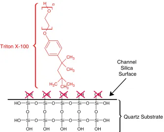
Figure 2.7 Triton X-100 Molecule . . . 42

Figure 2.8 Sodium Dodecyl Sulfate Molecule . . . 42

Figure 2.9 Surfactant Brushes w/o Silane SAM . . . 43

Figure 2.10 SDS Polymer Brush . . . 44

Figure 2.11 Triton X-100 Polymer Brush . . . 45

Figure 2.12 Electrokinetic Ion Transfer . . . 46

Figure 2.13 Trichlorosilane Molecules . . . 47

Figure 2.14 Atmospheric Chemcial Vapor Deposition Schematic . . . 48

Figure 2.15 Trichlorosilane Monolayer Chemistry . . . 50

Figure 2.16 Citric Acid Ionizations . . . 51

Figure 2.17 E. coli Illustration . . . 54

Figure 2.18 Bacteria Growth Phases . . . 56

Figure 2.19 Pile Area and Exclusion Zone . . . 59

Figure 2.20 PIV Flowchart . . . 62

Figure 2.21 Watershed Segmentation Example . . . 64

Figure 2.22 Moore Neighborhood Illustration . . . 65

Figure 2.23 Example Std Pile . . . 67

Figure 2.24 FSS Region Correlations . . . 68

Figure 2.25 Event Detection . . . 70

Figure 2.26 Example Liquid Layer Correlation . . . 72

Figure 2.27 Background Noise Correlation . . . 73

Figure 3.4 Péclet Number Analysis . . . 86

Figure 3.5 Autocorrelation example . . . 87

Figure 3.6 τL,τSdifference . . . 88

Figure 3.7 Péclet Number Analysis . . . 90

Figure 3.8 Permeability Analysis . . . 92

Figure 4.1 Microchannel Geometry Schematic . . . 98

Figure 4.2 E. coli Pile Time Series . . . 101

Figure 4.3 Bacterial Pile Formation . . . 103

Figure 4.4 Local Cell Orientation . . . 105

Figure 4.5 Cellular Orientation . . . 107

Figure 5.1 Shaped Particle Piles . . . 110

Figure 5.2 Electric Field Piles . . . 112

CHAPTER

1

INTRODUCTION

The goal of this dissertation is to experimentally investigate the formation of solids from microscopic

particles under the influence of pressure flows (flow-stabilized solids). Flow-stabilized solids provide a system to better comprehend colloidal and bacterial phenomena, specifically, the questions I seek

to answer can be generally stated as follows: how can colloidal and bacterial solids be characterized

with respect to their inherent fluctuations and what role does particle size and motility have on their formation? As a further consequence of the formation of bacterial solids, how does living

matter effect these solid piles? In this chapter, I will discuss the underlying physics that allows for

the formation of flow-stabilized solids (Sec. 1.1). Next, I will discuss the field of filtration and its major failure mode: filter fouling, which draws a direct parallel to FSS (Sec. 1.2). Next, I will review

the general fields of colloidal and active matter science (Sec. 1.3 & 1.4) in order to better understand

the particles used in my experiments. Finally, I will summarize the open questions I answer in this dissertation given the context provided by the literature review of Chapter 1 (Sec. 1.5).

1.1

Flow-Stabilized Solids

interactions. The main difficulty in this is the coupling of electrostatic and hydrodynamic forces

that effect both the particles and the fluid in which they are suspended. The following section will expand upon our current understanding of hydrodynamic aspects of this relationship and Sec. 1.3

will go into deeper detail with the electrostatic interactions. I will first introduce flow-stabilized

solids in Sec. 1.1.1 and provide physical context to where my experiments exist using dimensionless ratios. In order to understand the regime for which FSS exist, I will discuss the limiting case of fluid

flow the microfluidic channels Sec. 1.1.2, followed by the addition of particle suspensions into our

fluid flow, as seen in Sec. 1.1.3.

1.1.1 Flow Stabilized Solids

Flow-stabilized solids are a class of fragile matter that forms when a suspension of microscopic,

repulsive particles accumulates in an external fluid flow against a semi-permeable membrane. (Note that throughout this thesis, I interchangeably use the terms FSS or pile.) While prior work utilized

colloidal particles[Ort13; Ort14; Ort16], any repulsive particle with diffusive properties (thermal, active, etc) is capable of forming flow-stabilized solids. FSS only form above a critical flow rate[Ort13], as particle fluctuations will dominate particle motion below this critical point. From Ortizet. al.,

this is defined as the critical Péclet number, Pec. I utilize the Péclet number, the ratio of advection

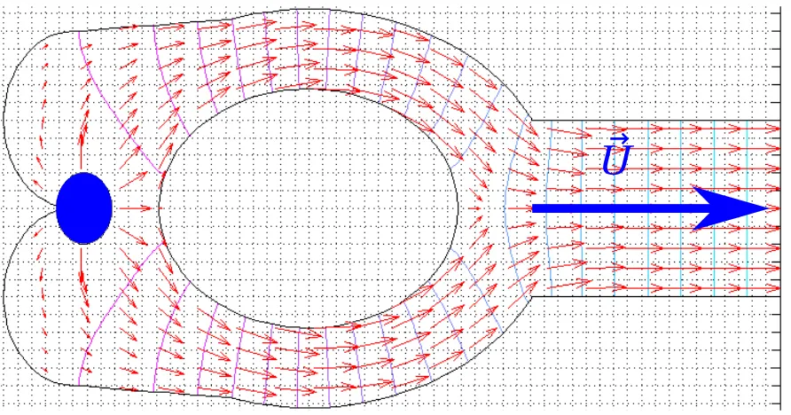
Figure 1.1Example flow-stabilized solid with 1040 nm microspheres at a steady-state. On the right half of the image, a fluid flow simulation is overlaid in red.

Fig. 1.1 is an example image of a FSS. Within in the pile, there are two distinct phases: the

solid phase, where particles are trapped within cages[WW02], and the liquid phase, where particle rearrangements can occur. Beyond the pile exists a gas phase, made up of the particle suspension, where particles can freely explore. After a pile has formed, if the flow is turned off or set below the

critical flow velocity, the FSS will dissipate back into the gas phase. The approximately triangular

shape of the pile in Fig. 1.1 is a feature of FSS, caused by a combination of shear (tangential) and compressive (normal) forces from the fluid flow, which is also shown in half of the image (the channel

is axially symmetric and the pressure differential spans the entire channel, therefore the flow field is

symmetric as well).

Flow-stabilized solids provide a model system to study microscopic solids, which are an

impor-tant phenomenon for fundamental understanding of the glass transition[Gok16; Wee16; VMS17; Gan18], dense suspension rheology[Che10; Hsi17a; Gho16; Sin19], particle confinement[Tei16; ZC16;

In order to provide physical context to the formation of flow-stabilized solids, I consider the

following set of dimensionless numbers and their approximate values for my FSS experiments. However, I first introduce the Navier-Stokes equations for viscious fluid motion[Tri12]:

∂ ~u ∂t =−

1

ρ∇p−u~· ∇u~+ µ ρ∇

2_u~+ 1

ρf~, ∂ ρ

∂t +∇ ·(ρ ~u) =0,

(1.1)

whereu~is the velocity field,t is time,ρis the density,µis the viscosity,p is the pressure, andf~is the applied body force. In the first equation, we can separate the right hand side into different forces

per unit volume: the pressure force, the inertial force, the viscous force, and the applied body force. The Reynolds number is the ratio of inertial and viscous forces inside a fluid,

R e=ρ ~u· ∇u~ µ∇2_u~ =

ρ ~u L

µ , (1.2)

whereLis the characteristic length. The Reynolds number was initially introduced by Stokes[Sto51], however it was later popularized for use in fluid mechanics by Sommerfeld and Reynolds[Som08; Rey83; Rot90]. For this thesis, I operate at low Reynolds (R e1), which will be more specifically detailed in Sec. 1.1.2.

Another important dimensionless parameter is the Stokes number, which represents the ratio of

the particle response time to the characteristic fluid time scale, when the fluid flow is held constant,

S t =τ0u0 l0

, (1.3)

whereτ0is the relaxation time of the particle with respect to particle drag,u0is the fluid flow velocity,

andl0is the characteristic length. For the low Reynolds number in this system,τ0=ρ

d2

18µ, whereρis the particle density,d is the particle diameter, andµis the dynamic viscosity. In physical terms, the Stokes number indicates whether particles will follow fluid flow streamlines. For my experiments, the

largest the Stokes number can be is∼10−8, therefore all particles will follow streamlines, excluding any additional forces beyond the fluid itself.

I utilize the Péclet number throughout the thesis as it is the ratio of advective (fluid) and diffusive

(particle) timescales. I defined the Péclet number as

P e=6πηr

2_u

kBT

, (1.4)

diffusion (Brownian motion) is central to the understanding of flow-stabilized solids. As the applied

pressure decreases, the diffusion of the particles will overcome the advection and a FSS is unable to form[Ort13]. As such, throughout my experiments, there is a range of Péclet numbers from 0.1 to 1000.

Given that FSS is a porous medium, it is useful to consider the Blake number. Similarly to the Reynolds number, the Blake number compares the ratio of inertial and viscous forces, but now

inside a porous media. The Blake number can be described as the Reynolds number for porous

flows:

B=uρDh

ηφ , (1.5)

whereuis the flow velocity,ρis the fluid density,Dhis the hydraulic diameter,ηis the dynamic viscosity, andφis the packing fraction. For my experiments, at maximum flow, the Blake number is on the order of∼10−2, therefore we can consider inertial forces to be negligible inside the FSS.

1.1.2 Hele-Shaw Microchannel

For our limiting case of a Hele-Shaw cell, which is a microchannel where the channel heightH and

lengthLare defined asH L, it is useful to reference the Reynolds number1.2 and the Navier-Stokes equations1.1, where we can consider the three separate forces of the Navier-Stokes equations: the

inertial force,ρ ~u· ∇u~, the pressure force,−∇p, and the viscous force,µ∇2u~. For our situation, in which the height of our channelH L, we consider a thin-film Reynolds number[Ach90]:

Re=ρU L

µ

_H

L

‹2

. (1.6)

In our experiments, we use at minimumH =1.5µm,L=14 mm,U =100µm·s−1. Therefore, we find a thin film Re∼10−8and can therefore consider the inertial term in the Navier-Stokes equation of motion to be negligible. This is more formally known as a Stokes’ flow[Kir10].

In the Stokes’ flow regime with our incompressible Newtonian fluid, our governing equations

become

µ∇2u~− ∇p+f~=0

∇ ·u~=0,

(1.7)

z

y

x

H

L

Figure 1.2This illustration represents a Hele-Shaw cell, which is a thin channel where fluid flows through. The channel is defined such thatHL. Curved edges indicate that the displayed width is not to scale. The coordinate frame setsx along the length of the channel (following the fluid flow direction),yalong the height of the channel (where the flow profile is determined, andzalong the width.

Due to the fact thatH W and that our flow remains in a steady-state (∂_∂p_t =0), we can consider

the fluid flow as two-dimensional. If we consider a small fluid section within the flow, we can

compute the net viscous force acting on it in the y-direction:

∂ ∂y



µ∂u ∂y

‹

=µ∂2u

∂y2. (1.8)

Furthermore, the net pressure force acting on the fluid section in the x-direction is

−∂p

∂x. (1.9)

Given our steady-state flow, we can assume that the flow profile remains constant throughout the channel and therefore the pressure gradientG is

p1−p2

L =− ∂p

∂t =G, (1.10)

and thus the momentum of the fluid element is not changing as it moves downstream. Therefore

the total force acting on the fluid element is zero and we arrive at the following relation:

µ∂2u ∂y2 =

∂p

or,

µd2u

d y2 =−G. (1.12)

Integrating, our velocity profile now takes the form of

u= G 2µ(a

2

−y2), (1.13)

which is parabolic in nature, and therefore a Poisseuille flow.

1.1.3 Particle Suspensions in Microchannels

Analytical particle suspension solutions of the fluid flow in Hele-Shaw cells is a complex problem, involving the combination of hydrodynamic flows, particle to particle interactions, and channel to

particle interactions (all of which couple both electromagnetic and hydrodynamic interactions).

Solutions to this situation have been considered by numerous studies ranging back almost a century ago[Fax22]to more recent studies, which broaden our understanding different types of particle suspensions[Bet18; Poz94; Alv06].

For our experimental situations, we consider only the limiting cases and their effect on stream-lines, field lines in a fluid flow, for the bulk fluid and particle suspension. The main takeaway from

considering this limiting case is recognizing the difference between a 3D regime and a quasi-2D

regime. This confinement breaks the correlations from a monopole contribution (1/r) to a dipolar contributions (1/r2_).

(a) (b)

field of the following form exists, as seen in Fig. 1.3[Cui04]:

vx,y,z(r) =

 _F

p 6πηH

‹

∆x,y,z(r), (1.14)

where Fp is the force exerted on the fluid by a moving particle,ηis the fluid viscosity,H is the distance between the top and bottom of the channel, and∆is given by

∆x(r) =h(y)

x2−z2

(x2+_z2)2

,

∆z(r) =h(y)

 _{2x z} (x2+_z2)2

‹

,

∆y(r)∆x,z,

(1.15)

withh(y) =−94y2+ 9

16H2representing the contribution of the parabolic flow profile (Eq. 1.13). At the

top and bottom of the channelh(±H/2) =0. Note that I am utilizing the coordinate frame shown in Fig. 1.2.

1.2

Filter Fouling

Flow-stabilized solids provide a novel model of a simple filter membrane due to the channel

geom-etry utilized to form FSS. In the microchannel, a barrier is placed perpendicular to the flow. The

barrier is shorter in height than the channel walls, creating a gap which allows fluid to flow over the top of the barrier, but not particles. This geometry is analogous to a filter membrane since fluid

flows over the barrier ("single-pore" membrane) and the gap above the barrier does not allow

con-taminants to flow over it. These solids are formed through a combination of compressive (dead-end filtration) and shear (crossflow filtration) forces, allowing me to extend the filter model to both types

of filters. The FSS, which forms on the barrier, is dependent upon a sufficient flow rate[Ort13]and is therefore analogous to the formation of cake on the membrane surface, which is integral to our understanding of filter fouling.

In this section, I will provide background context and history of advances and problems seen

in the field of filtration (Sec. 1.2.1). From this context, the topic of filter fouling can be considered (Sec. 1.2.2) and then related to flow-stabilized solids. Specifically, further analysis on the so-called

1.2.1 Filtration Overview

The first recorded instance of microporous membrane is by Zsigmondy in the early 1900’s[Zsi22], who patented the idea in Germany. Zsigmondy utilized our understanding of osmosis[Nol48], diffusion[Fic55], colloids[Gra61a], and osmotic pressure[Tra67; Pfe77; Hof87; Hof88]to create a contaminant removal system. Beyond Zsigmondy’s initial filter, a number of different researchers extended this initial idea[Lon82]and by the 1980’s filtration science and technology had extended into our current modern age, with nanofiltration (NF), ultrafiltration (UF), microfiltration (MF), and

reverse osmosis (RO).

These three techniques help categorize almost all of the membrane filters used in both scientific

and industrial settings. Nanofiltration, ultrafiltration, and microfiltration are similar in their

funda-mental methods, in that fluid flows through a membrane, separating out contaminants and leaving behind a fouling cake layer of undesirable particulate matter. Reverse osmosis differs from NF, UF,

and MF in that it utilizes osmosis to move fluid through the membrane instead of a dependence upon an applied pressure. I will mainly focus on microfiltration, given that its operating parameters

(a) (b)

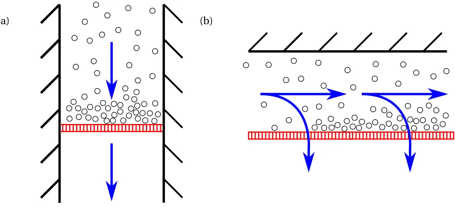
Figure 1.4An illustration of the two most common filtration types: (a) dead-end filtration and (b) cross-flow filtration. In each image, walls are considered impenetrable, fluid cross-flow is indicated by blue arrows, particles are shown as black circles, and the membranes are in red. In dead-end filtration (a) the mem-brane fouls in the direction of the flow, directly impeding the flux of the filter. In crossflow filtration (b) the membrane is perpendicular and parallel to the fluid flow and therefore fouls at a slower rate.

There are two membrane filter modes: dead-end filters and crossflow filters (illustrated in Fig.1.4). Dead-end filters are the simpler design of the two, utilizing a single channel or pipe flow,

with a membrane perpendicular to the fluid flow separating out foulants from the fluid suspension.

However, since both fluid and contaminants flow through the same membrane, filter fouling occurs quickly as a cake layer forms and lowers the overall filter flux. In the 1960s, Sieveka[Sie66]discovered that flowing the fluid suspension parallel to the membrane caused in increase in permeation flux,

and thus an increase in the overall performance of filters.

Today, in most industrial settings, crossflow filtration is utilized in the place of dead-end filtration

due to its increased performance, with most dead-end filters seen in simpler settings. In these

industrial settings, filtration is used to aid in sterilization, water treatment (more commonly in association with membrane bioreactors (MBR)), oil refinement, isolating biological cell cultures, and

other purification methods. However, for all of these methods and uses, filter fouling is a persistent

and major failure mode[Bel94; Lee01; Pan05; Wan05; Bac06; Guo12].

1.2.2 Filter Fouling

Filter fouling is defined as the loss of permeation flux across a membrane filter; it is important to

fouling[Guo12]. For flow-stabilized solids, the fouling is reversible because the pore cannot be plugged. Furthermore, the foulants I consider in this thesis are colloids[LB03; Ken03; Hua08](Sec. 2.3) and microbiological organisms[Ivn05; Vro10; Xu10](Sec. 1.4), which make up a large percent of industrial and scientific fouling situations. It should be noted, that the maturation of biofilms is a

component in the fouling of filters by microbiological organisms[Gha96; WK00; NP07; Vas14], my formation of FSS with bio-organisms does not have biofilm formation. However, even without the

formation of biofilms, biocake[Lee01]accumulation in MBRs are a significant problem due to the added variables involved with living foulants instead of inanimate particulate matter[Pan05; Wan05; Xia14]. A further discussion on this topic is in Sec. 1.4.

A number of modifications to the flow and filter channel have been proposed and

experi-mented on, including inducing flow instabilities[KN85; Kro87; GS09], adding roughness to the channel[Tho73; CM91; Sch03; Chi06], flow oscillations[Ken74; Bau82], and applying external EM fields[Aka10; BME10; Wei11a; Wei12; Wan13; Haw15]. However, these processes simply attempt to mitigate the onset of filter fouling instead of understanding the fundamental mechanisms associ-ated with this failure. One such approach is through the concept of critical flux, first introduced by

Field[Fie95], which can be defined the flux at which fouling becomes noticable or the flux at which irreverisible fouling occurs[Bac06].

1.2.2.1 Critical Flux

Given that Bacchin’s review of critical flux[Bac06]included multiple definitions of critical flux, there have been more recent studies attempting to clarify what critical flux actually entails[AB10; FW11] or rather that there exists a family of critical fluxes[FP11a]. Included in this family of critical flux definitions is limiting flux[Bac04], which is defined as the point at which flux begins to decrease across the membrane; but there are at least two different models for this behavior[Tan09]. Another member of this family of definitions is the sustainable flux, which is more of an economical approach

to flux, which includes the cost to maintain a flux in an industrial setting[Fan07]. For the scale of the flow-stabilized solid experiments, I consider only the critical flux with respect to the formation of a

cake layer (and thus the formation of FSS) and with respect to the transition to an irreversible cake

layer (and thus the transition from a thermal to athermal region; see Chap. 3).

In order to provide context to the critical flux idea with respect to flow-stabilized solids, it is

useful to consider Field’s original discussion on critical flux[Fie95], which considers the critical flux hypothesis

behavior[Bac95; Mcd89; Bow96; Bac02; BC95; Bha99; JJ96; Pet93; PZ94; HA96; Bow99; BS02; KZ04; SE95], it is difficult to pin down an exact mathematical set of statements for when the critical flux occurs. However, from a physical characteristic standpoint, the critical flux is considered to be a

loss of force balance between drag forces and dispersive forces, such that particles begin to deposit

on the surface.

From this definition, a direct correlation has been made to the Péclet number (see Eq. 1.4). Initial

use of the Péclet number for particulate deposition on membrane processes begins in the early

1900’s[ST36], and continued as membrane technology advanced[Bir60; Bha97; MH99]. A relation between the critical flux and the Péclet number was first published by Bacchinet al[Bac04; Bac06], who suggested that a critical Péclet number could identify the initial point of membrane fouling.

This idea has also been extended to gas separation membranes[Nag13; NH14]. A more recent study, which included experimental verification, by Zamaniet al[Zam14]considered a modified critical Péclet number:

Pecrit=

_J

crit(x)δc Ds

‹

, (1.16)

where Jcrit is the critical flux,δc is the concentration boundary layer thickness,Ds is the shear-induced diffusion coefficient, andx is the distance along the length of the filter membrane (see Fig. 1.5). Fig. 1.5 from Zamaniet al’s study helps illustrate the situation in a crossflow microfiltration

setup with respect to the critical Péclet number.

From this critical Péclet number, the further conclusion can be made that as the Péclet number

passes its critical point atx, particle deposition occurs and cake begins to form on the membrane. For my experiments, the main transport mechanisms which are modeled by filtration studies

are Brownian diffusion

J_{B D} =1.31

γwDB D2 L

φw φb

1/3

, (1.17)

(whereγwis the shear rate at the wall,DB Dis the diffusion from thermal fluctuations,Lis the channel length, andφw,b is the packing fraction of the cake and bulk suspension respectively)[TD80]and shear-induced diffusion

JS D=0.078γw

r4 L

1/3

ln φ w φb ‹ , (1.18)

wherer is the radius of the cake particles[ZC86]. Note that from a granular physics perspective, shear-induced diffusion is similar to stick-slip avalanching.

There is a clear connection between our flow-stabilized solid’s critical Péclet number[Ort13] and the reversible critical flux, given that both indicate the initialization of solid formation on a membrane. Further discussion on this relation is in Chapters 3 & 4. For the colloidal experiment,

I consider the reversible critical flux from the standpoint of different colloidal particle (Sec. 1.3)

sizes in an attempt to find a universality for this critical point. Additionally, I discuss a thermal to athermal transition in the FSS, which hints at a connection to the irreversible critical flux. For

the bacterial experiment, I modify the Péclet number by replacing the diffusion with stochastic

motility of run-and-tumble bacteria to handle the active matter (Sec. 1.4) component of the bacterial particles and see a similar connection to the reversible critical flux. Additionally, I see the added

variable of cellular reproduction in our experiments, which draws a connection to failure modes

seen in membrane bioreactors.

1.2.2.2 Cake Formation

Cake formation on filter membranes inhibits the main goal of filter use: to separate out contaminants

from a suspension. As the cake deposits onto the membrane, the fluid has added obstacles toward

its motion through the membrane. Flow through cake follows Darcy’s law of fluid flow through a medium[Bel94]:

J = 1 A

d V d t =

∆p η(Rm+Rc)

, (1.19)

Carman-Kozeny equation gives[Car38]

Rc =K0·

‚ φ2_S2

p

(1−φ)3

Œ

. (1.20)

K0is the Kozeny constant, which is typically set to∼5[Gra53]andSpis the shape parameter of the particles, which is the surface area per volume of each particle (for spheres it is 3/r). For compressible cakes, a power law relation has been proposed to define the cake resistance[Por77; Bel87; Bel94; Sio10]

Rc=m·β(∆p)s, (1.21)

whereβis an empirically determined constant andm is the mass load (mass per unit area) of the cake. Ass approaches 0, the cake is incompressible. Due to the decreased permeability of fluid flow,

the flux across the membrane is greatly reduced[Shi05; CL06; JL07; Ram07; Wan07; Men07]. In addition to the decreased permeability, another effect of the densely packed particles is the increased ion concentration, which is causes an increase in the opposing osmotic pressure

across the membrane. This is called the cake-enhanced osmotic pressure[HE03]and has been experimentally and numerically verified for both colloidal[Ng05; Cho07; Wan07; CF09]cake as well as biocake[Cho08]. Between these two effects, we can see that the formation of cake has a significantly inhibiting effect on the efficiency of filtration systems.

1.3

Colloids

Colloids are a dispersion of one phase of matter into another phase of matter. This thesis focuses

on solid dispersions in a liquid medium, however, colloids can take the form of foams (gas to

solid/liquid), aerosols (liquid/solid to gas), emulsions (liquid to liquid), and gels (liquid to solid). There is no general consensus on the exact definition on colloid size, but in general these particles

range in size from 10 nm to 10µm. Particles larger than the upper bound of colloids are considered to be granular materials; these particles are not subject to thermal fluctuations. Particles below the

lower bound can be molecules, single atoms, proteins, or other nanometer-sized particles.

Colloidal suspensions are a mixture of insoluble microscopic particles in a suspending medium, typically in the form of solid particles and liquid medium. The study of colloids and colloidal

(metals & inorganics) to be crystalloids. While his definition of colloids did not survive to our

modern studies due to his exclusion of low molecular weight suspensions, it did influence the work of Weimarn[Wei11b], Ostwald[Ost12], and Freudlich[Fre30]who arrived at a more encompassing definition of what a colloid is: any molecule which is insoluble in an aqueous suspension and is

influenced by Brownian motion (Sec. 1.3.2).

In this section I will discuss the modern view of what a colloids and colloidal suspensions are, as

well as their scientific and industrial importance (Sec. 1.3.1). Next, I will look into the main internal

driving force for colloids: thermal fluctuations under the direction of Brownian motion (Sec. 1.3.2). Finally, I will discuss physics of intercolloidal interactions (Sec. 1.3.3), which are associated with the

stability (whether a colloid flocculates or sediments) of colloids and more specifically determine the

viability for experimentation. Sec. 1.3.3 discusses the forces at play within the colloidal experiments 3; as such, the physics described is viewed from the lens of the experiment’s particular specifications.

Further discussion on the specific material and chemistry choices can be located in Sec. 2.2 &

Sec. 2.3.

1.3.1 Colloids Overview

Colloids are subject to thermal fluctuations (Sec. 1.3.2 and exhibit a Lennard-Jones like potential

that is attractive near the surface and repulsive as the separating distance between two particles increases. This provides a similarity to atomic models[Man15], which was famously utilized by Einstein[Ein05]to estimate the size of atoms (for which he earned a Nobel Prize in 1926). This can be further utilized to study atomic phenomenon, such as the glass transition and crystallization kinetics[Poo04]. Due to the broad size range and the tunable potential associated with colloids, they are widely used in industrial, where they take the role of both products (such as shampoos,

detergents, food products, paints) and methodology enhancers (such as drug delivery[Kre14], oil recovery[PM01], biomolecules[Ela03]). In contrast to their positive benefits, they are also a major causing of filter fouling (discussed further in Sec. 1.2). Ultrafiltration, microfiltration, and reverse

osmosis are all industrial scale methods for removing contaminants from process liquids (such as decontaminating wastewater); however, fouling by colloids or other like-sized particulate matter

decreases the filter efficiency (flux permeation) and can irreversibly clog filter membranes.

For the purposes of this thesis, the colloids to be studied are in a mesoscopic range (∼0.5µm−

1.3.2 Brownian Motion

A single colloid in a suspension medium, which is at rest, will undergo random motion, which is known as Brownian motion, named after botanist Robert Brown[Bro28]. Brownian motion is driven by collisions between the fluid molecules and the colloid[Fey64]. For a single particle in a suspension, the Einstein-Stokes-Sutherland relation[Ein05; Sut05]is as follows:

D= kBT

6πηr, (1.22)

wherek_BT is the thermal energy,ηis the viscosity of the suspension medium, andr is the radius of the spherical colloid suspended in the medium. Note that traditionally, the relation is called

the Stokes-Einstein relation, however Sutherland published a derivation of the same relation a few months before Stokes and Einstein published their own paper. This relation gave rise to the

fluctuation-dissipation theorem, which was proposed by Harry Nyquist[Nyq28]in 1928 and proven by Herbert Callen and Theodore Welton[CW51]in 1951. The fluctuation-dissipation theorem states that for any process which releases energy (such as particle drag in a viscous fluid) as heat and has a

reverse process related to thermal fluctuations (such as Brownian motion). For Brownian motion,

this gives rise to the following relation for the diffusion constant with respect to the average mean squared displacement[Kub66]:

〈(x−x0)2〉=2D t, (1.23)

which therefore means that the diffusivity of a particle is defined by the viscosity of the suspension

medium.

1.3.3 Colloidal Stability

For colloidal suspensions, the interactions between particles and surfaces (in our case, focusing on particle to particle and particle to surface interactions) is of major significance to the transport

and stability behavior of the colloids in the suspension. Colloidal stability is defined as particles

remaining suspended in solution without floccuating or forming sedimented layers.

For our experiments of monodisperse, quasi-2D colloidal suspensions, sedimentation does

not occur in a destabilizing manner, as the particle population sediments at a singular rate and is

counteracted by the Brownian motion of the particles. At low Reynolds number, the sedimentation velocity is given by the a ratio of gravitation forces and the Stokes drag[Fel05]:

v=2 9

∆ρr2g

η ≈1.46×105·r2, (1.24)

acceleration, andηis the fluid viscosity. Given our colloidal microspheres radii range of∼.5−1µm, the sedimentation velocity is on the order of 100 nm·s−1, which is at least an order of magnitude below our experimental velocities. Furthermore, the diffusion rate of the particles is on the order

of 0.25µm2·s−1, which, in combination with the quasi-2D channel geometry, suppresses most of the sedimenting effect in the channel. As such, for our experiments, we consider only flocculation (aggregation) with respect to our colloidal stability. (It should be noted that sedimentation in the

inlets causes a slight increase in channel suspension density, however, we choose a low enough

suspension density at the start of each experiment that the increase in suspension density during the experiment only effects the rate of pile formation, not the steady-state pile itself.)

A modern comprehension of colloidal destabilization due to aggregation began with the

formu-lation of the DLVO theory (Sec. 1.3.3.3) in the mid 1900’s[Rus89], which was a collaborative effort of Derjaguin, Landau, Verwey, and Overbeek to combine the respective attractive and repulsive

electrostatic effects of the van der Waals force (Sec. 1.3.3.1) and the electric double layer (Sec. 1.3.3.2).

This formulation includes the effect of the suspension’s ionic concentration on the colloidal stability, which was a failure of the Levine-Dube theory[LD39; LD40]. In addition to DLVO forces, which are electrostatic in nature, colloidal suspensions can also destabilize due to the following[Gra02]: hydro-gen bonding energies, hydrophobic interactions, solution chemistry (Sec. 2.3.4), depletion forces (Sec. 1.3.3.4), and surface roughness. I treat the polystyrene particles with surfactants (Sec. 1.3.3),

therefore the hydrogen bonding issues caused by differing functional groups on the surface can be ignored[MF78; FM78]. These functional groups also inhibit the effects of polystyrene’s hydropho-bicity[Thr08; Li07]and roughness[Kaj97]. A more explicit discussion of interaction energies in the context of our experiments is discussed in Sec. 2.3.

1.3.3.1 Van der Waals Force

The van der Waals force is an attractive electrostatic force, which has non-negligible effects only at nearby particle to particle (or particle to surface, etc) interactions, typically on the order of 10 nm

or less. It is a major factor in colloidal instability, as salt concentration dictates whether attractive

or repulsive forces dominate body to body interactions[Szi14]. While its initial formulation by van der Waals in his PhD thesis was within a vacuum medium and under the assumption of pairwise

additivity[Waa73], it has been extended to a breaking of pairwise additivity[Lif54; Lif58]and further discussion on handling non-vacuum mediums is shown below.

The van der Waals potential form follows the typical pair potential formulation, such that

the attractive van der Waals decreases rapidly as the interaction distanceD increase. However, it

was further determined that the decrease in attractive force strength changes more rapidly than 1/r6_{[CP48]. The main importance here is that beyond the initial zone of attractive force from the}

van der Waals force, other forces will quickly dominate.

x

D

x

=

0

R

z

z

=

0

z

=

2

R

Figure 1.6Van der Waals force illustration with an infinite surface (red) and a nearby spherical particle (blue). The particle and surface are separated by a distanceD. The particle has a radius ofR. Two 1D coordinate systems are shown: ˆxdescribes the distance from the surface; ˆzdescribes the distance from the farthest left point on the sphere.

If we consider the situation illustrated in Fig. 1.6, where a spherical particle, with radiusR,

approaches a surface and is separated by a distanceD, and utilize chord theorem[Coe69]to set x2_{= (2R−z)z, we can see that the work done on the particle is given by}

W(D) =−2π

2_C2

ρ 6

Z 2R

0

(2R−z)z d z

(D+z)3 . (1.26)

When we letDR, the work simplifies to

W(D) =π

2_C2

ρR

6D . (1.27)

For a vacuum medium, we can use the Hamaker constant[Ham37]to help simplify interparticle body to body interactions:

whereC is the interaction parameter from the van der Waals pair potential andρi is the particle densities of the two interacting bodies. Due to the assumption of a vacuum medium, the interaction potential provided by the Hamaker theory[Ham37]for two spherical particles varies from aqueous mediums[NP71; Smi73; TGR01]. However, it is standard procedure[Gut07; JB12; BR13; BR14; Kop17] to determine the Hamaker’s functional form for the required geometry and then insert an experi-mentally determined value for the Hamaker constant. Our relevant body to body interactions are

sphere to sphere and sphere to surface, which have the following work relations[Isr11], respectively,

W(D) =−A 6D

 _R

1R2

R1+R2

‹

,

W(D) =−AR 6D .

(1.29)

The radii term for sphere to sphere interactions is known as the effective radiusR_eff= R1R2

R1+R2

.

1.3.3.2 Electric Double Layer

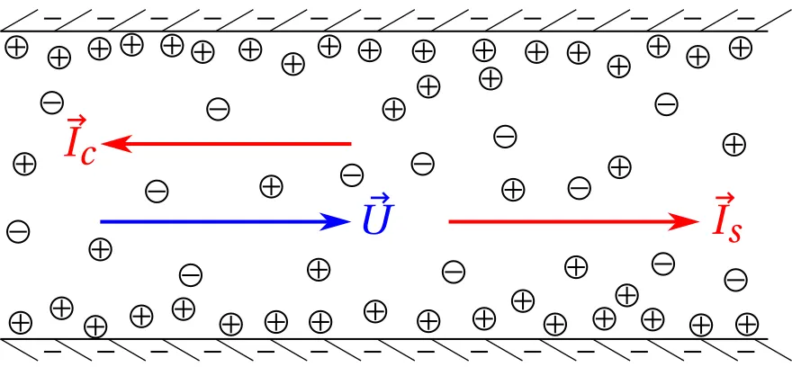
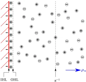
The electric double layer is the combination of parallel layers of charge on a surface (typically

in an aqueous solution): the first layer is the surface charge (also known as the inner Helmholtz

layer[Hel53]), which consists of absorbed ions on the surface; the second layer is a more diffuse layer of ions attracted the surface charge by electrostatic attraction. The second layer is the outer

Helmholtz layer (OHL), which completes the electric double layer and thus Helmholtz’s description

of a molecular dielectric which stores charge and repulses like charge nearby. The following is an adaptation from Leal’sAdvanced transport phenomena : fluid mechanics and convective transport

processes[Lea07].

In order to solve for the electrostatic effect from the electric double layer, we consider this geometry within the context of a typical electrostatics problem. Poisson’s equation for electrostatics

states the following partial differential equation for an electric potential:

∇2ψ=− %

ε0ε

, (1.30)

whereψis is a scalar electric potential field,%is the ion charge density,εis the permittivity of the medium, andε0is the permittivity of a vacuum. If we consider the illustration in Fig. 1.7, where we

have a negatively charged surface and near a diffuse solution of cations and anions, we can view

IHL

OHL

_κ

ρ

Figure 1.7Illustration of the electric double layer at a surface in a suspension of ions. The inner Helmholtz layer (IHL) and outer Helmholtz layer (OHL) are indicated near the negatively charged surface. The Debye lengthκ−1_{is indicated by a dashed line and as the distance from the surface increases to the bulk solution,} the ion concentration becomes%_∞. At%_∞the cation and anion concentration is equivalent. Near the surface, there are more cations than anions.

Therefore,

∂2_ψ

∂x2 =−

% ε0ε

, (1.31)

with the boundary condition that in the bulk solution, when%=%_∞,ψ_∞=0. Therefore the work required to move an ion fromx→ ∞isz_ieψ_x. In order to determine the charge density%from the Poisson equation, we consider the number density of ions at the edge of the OHL (see Fig. 1.7)

within the context of a Boltzmann distribution, such that

ni=ni∞e(

−zi eψx kB T

Š

We now have a more physical description for the Poisson equation, noting that%=P

i

zie ni,

d2ψ d x2 =

−e ε0ε

X

i

z_ini∞e

€_{−zi eψx}

kB T

Š

. (1.33)

We can expand the exponential via a Maclaurin expansion in order to reach the Debye-Huckel approximation, which states the surface potential should be small enough such that

zieψx k_BT

<

1. (1.34)

This assumption holds for low ion concentrations that are within the regime of the DLVO theory

(see Sec. 1.3.3.3)[Bos01]. Therefore the exponential can be approximated to two terms: 1−zieψx

kBT .

Given our earlier assumption of a bulk electroneutral solution, which is how we state thatψ_∞=0, we see thatP

i

zie ni∞=0. Thus,

d2_ψ

d x2 =

−e2

ε0εkBT

X

i

z_i2ni∞ψx. (1.35)

To further simplify, we define

κ2₌ e2

ε0εkBT

X

i

z_i2ni∞, (1.36)

whereκ−1represents the measure of electrostatic effect from the surface charge, which is known as the Debye length. We can utilize the relation of ion number density with respect to molarity

(ni∞=NA·ci∞), to relate the Debye length to the molar concentration of the suspension in order to arrive at a physical situation for the Debye length, which for electrolyte solutions is on the order

of nanometers. With our simplification and the boundary conditions ofx →d :ψx →ψd and x→ ∞:ψx→0, we arrive at the solution to our electric potential as

ψ=ψde−κ(x−d). (1.37)

A further expansion of the electrostatic properties is used for Sec. 1.3.3.3, in which we find that the

surface charge density is given by

σd=−ε0ε

dψ d x d =p

8kBTε0εni∞sinh

_z

ieψd 2kBT

‹

due to the exponential decay of the force asx→ ∞. Similarly to Sec. 1.3.3.1, we can simplify the

energy interaction base on our two experimental situations: sphere to sphere and sphere to surface, respectively

W(D) =Reffzie−κD,

W(D) =R zie−κD,

(1.39)

where we again utilize the effective radius defined byR_eff= R1R2

R1+R2

.

1.3.3.3 DLVO Theory

The combination of the van der Waals force and electric double layer was proposed as a means

to explain the interparticle potential in aqueous suspensions by Derjaguin[Der39], Landau[DL41], Verwey and Overbeek[VO48]. Following our discussion from Sec. 1.3.3.3 and 1.3.3.2, DLVO theory assumes that we can approximate the interaction of two particles to be additive with respect to van

der Waals forces and the electric double layer:

WD LV O(D) =Wv d W(D) +WE D L(D). (1.40)

For the case of any two surfaces, we then see that

WD LV O(D) =− A 12πD2+

2σl e f tσr i g h t ε0εκ

e−κD, (1.41)

whereσis the surface charge density of the left or right surface, which is given by Eq. 1.38, andκ−1

is the Debye length, which is given by Eq. 1.36. In order to understand the suspension interparticle

interactions, we consider the sphere to sphere case, where we have the following interaction free energy[Bha98]:

WD LV O(D) =− A

12πD2+64πkBT R%∞κ

−2_e−κD_tanhz eψ0

4kBT

‹2

, (1.42)

where%_∞is the ion number density in the bulk solution,z is the valency of the ions, andψ0is the

surface potential on the surface.

1.3.3.4 Depletion Force

Outside the realm of DLVO forces, an additional destabilizing force for colloidal suspensions is the

the flocculation and added attraction between particles. It should be further noted that failure to

completely eliminate depletion forces (or at least compensate with other particle interaction forces) within a colloidal suspension changes the hydrodynamics of the suspension[Cro99].

R

R

_m

D

Figure 1.8Two spherical colloids of radiusR, in blue, separated by a distanceD. Micromolecules of radius Rmare present in the solution. The micromolecules cannot enter the separation region between the two

spheres ifD<Rm.

An illustration in Fig. 1.8 represents a zoomed-in view of a suspension situation between two microspheres, with radiusR, with micromolecules, also known as depletants, (RmR) present in

the medium. In the case where the micromolecule concentration is too high, the microspheres will feel an attractive pressure (known as the depletion force) equivalent to the osmotic pressure[Isr11]

PD=Po=−%kBT. (1.43)

For a microsphere separationD<Rm, we consider the work done on the particles by the attractive pressure[AO54; AO58]

W(D) =− Z D

Rm

P(D)d D=−%R_mk_BT

_1−D

Rm

‹

for two spheres[Vri76], we have the depletion force defined as

F(D) =πRW(D) =−πR Rm%kBT

_1−D

R_m

‹

, (1.45)

therefore,

W(D) =− ZD

Rm

F(D)d D=−1

2πR R

2

m%kBT

_1−D

Rm

‹2

. (1.46)

In order to characterize this effect within the context of micromolecular concentrations, we consider

the following approximation of the micromolecular volume fraction

φ≈%R_m3, (1.47)

where can only assume the micromolecule will be three dimensional, but know nothing about its

shape. However, we can still determine an order of magnitude measure of the work done by the depletion force by inserting our volume fraction:

W(D)≈ −1

2π R Rm

φk_BT

_1−D

Rm

‹2

. (1.48)

From this we can determine whether we can either shield the particles from depletion force effects

with a polymer brush on the surface of particles whose lengthL>Dor whose electrostatic shielding effect creates a repulsive force greater than the depletion force.

1.4

Active Matter

Active matter is nonequilibrium condensed matter that is composed of self-driven units, which are capable of converting energy into motion[Sch07; Mar13]. This broad definition is well-suited for active matter, as it is studied throughout a variety of scientific fields: statistical physics[Ram10], biology[Vis11], robotics[Bra13], soft matter[Mar13], biomedicine[WG12]. From these fields a wide range of applications are being developed[Bec16]such as personalized health care[Nel10; WG12; Pat13; Abd14], environmentally sustainability[GW14], and lab-on-a-chip chemistry[Ebb16]. This has given rise to a number of studies on active matter, which is illustrated by the sheer number of reviews on active matter in the last decade[JP09; Ram10; Cat12; Ton12; Mar13; Men; Elg15; ZS16; Bec16; Zer17].

is discussed in this thesis, typically is associated with fluid flow at low Reynolds number, where

inertial effects are negligible. Wet active matter examples include any motile microorganism and active Brownian particles, which are sufficiently small to conserve their momentum.

1.4.1 Active Hydrodynamics

Given thatE. coliis the most studied bacterium[Ber03], I choseE. colito be the bacterial suspension used in my bacterial flow-stabilized solid experiments (Chap. 4). The bacterium undergoes run and tumble motion, in which during the run section, it swims in a straight line (at aroundve c o l i=

20µm·s−1[Cat12]). After completing its run, the bacterium tumbles randomly, until a new direction of motion is determined. This tumble motion is then repeated indefinitely. The run-and-tumble event rateα(how often a motion cycle is completed) is dependent upon the Brownian diffusion of the bacterium, in that evolution dictates that the run portion is completed before the time scale of the bacterium’s rotational diffusion,τB[SL10]. The run-and-tumble motion is a stochastic process, due to the randomness of the tumble portion, therefore, we can model the

motion within the context of a run-and-tumble diffusion

DRT = v_{e c o l i}2

αd , (1.49)

wheredis the dimensionality of the motion.

In addition to considering the run-and-tumble diffusion, it is important to reassess the

effec-tiveness of the Péclet number, which does not include the effect of active motion. We can define a

modified active Péclet number[ZS16]

PeA=

2R ve c o l i DRT

, (1.50)

whereRis the radius of the particle (in the case of a sphere),ν0is the velocity of the particle with

respect to its self-propelling, andDis the diffusion coefficient of the particle. A further modification

considers the persistence number[Fri08; LT09; Tak11]

PeR= ν0τR

2R = L

2R, (1.51)

whereτR is the persistence time (the time a particle persists in a single direction of motion), and Lis the persistence length (the distance travelled by a particle’s self propulsion before it changes

motion[RS15; PK92]such that

~

V =ν0e~+v~(r~(t)), (1.52)

wheree~is the orientational vector of the particle, andv~is the velocity of the flow field. Furthermore, the angular velocity is then given by

~

Ω=1

2∇ ×v~+

γ2₋₁

γ2+₁

~

e×E·e~, (1.53)

whereγis the aspect ratio of the particle (γ=l/w), andEis the strain rate tensor. From these, we arrive at the following equations of motion for an active particle in an external flow field:

˙

~

r =ν0e~+v~,

˙

~

e =Ω~×e~. (1.54)

These equations of motion are known as Jeffery orbits, which are named after George Barker Jef-fery[Jef22]. They are known as orbits due to the fact that they describe the irregular rotation of ellipsoids in shear flow.

As an active particle in an external field approaches a wall (as with the initial formation of flow-stabilized solids), the dynamics become increasingly complicated. Fig. 1.9 from[ZS16]illustrates the complicated dynamics involved at a wall interface. For my experiments,E. coliapproaching a

Figure 1.9From Zöttl and Stark[ZS16]. (a) Collision of an active colloid with a surface: collision at timet0, reorientation close to the wall, and escape from the wall at time t. (b) Definition of the coordinate system for an active colloid swimming in front of a wall: distance from the wallhand orientation to the wallθ. (c)-(g) Reorientation mechanisms close to the wall contributing to its angular velocityΩW,φ=θ˙: rotational noiseΩN(c), hydrodynamic swimmer-wall interactionsΩH(d), which can depend on the chemical field c(r)(e), external fluid flowΩF (f ), and steric interactionsΩS(g).

Beyond the single particle comprehension ofE. coli, analytical solutions for the hydrodynamic

interactions for fluid-particle and particle-particle are difficult to determine[Cat12], however these interactions can be modeled based on approximations or ignored due to having no effect on the suspension. For systems in thermal equilibrium, the fluid-particle interactions have no effect on

steady-state densities[DiL05; Hil07; TL08; Nas10]. Particle-particle interactions have a potential form of 1/r2_{[LP09], and therefore have minimal effect at non-near separations. Furthermore, this}

interaction is weak and can be overpowered by the background noise in the system[Dre11]. Bacteria motility is dependent upon suspension density, whether due to collective motion[Zha10; Hen11; Ton12], biofilm formation[HSC04], or crowding[Nas10]. In order to model the density field of a dense bacterial suspension, one can utilize the probability density from the Fokker-Planck

and living matter. Inanimate active matter, such as self-propelled colloids, can serve as a model for

understanding their living counterparts[Zer17], however, they lack specific properties which would allow us to more directly compare them to living matter.

From Schrödinger, Eigen, and Dyson[Sch43; ES77; ES78; Dys82], we have the following three properties: self-assembly, self-replication, metabolism, which are required to be considered living at the microscopic level. There has been significant work attempting to let colloids exhibit each of these

properties[Zer17]. Controlled self-assembly is achieved through specific interactions, which are a means of transferring information, such as DNA-mediated interactions[Bia05; Dre09; AU14; The13]. Self-replication is a complicated behavior, which can be handled from the viewpoint of replicating

colloidal clusters, using a surrounding suspension of colloids[ZB14]. Dyson[Dys82]argued that metabolism, which is a cascade of complex chemical reactions, is the most critical aspect of living systems. Metabolism for colloids has been shown to be possible with templated reactions of colloidal

clusters, which then cascade[ZB17].

This discussion of attempting to simulate life-like features with colloids skirts around a deeper topic: our understanding of biology, specifically, micro- and cellular biology, from a fundamental

physics level, is lacking. The emergence of biophysics in the last few decades has given rise to a

significant number of collaborative efforts between biologists and physicists; however, these group efforts have also seen an increase in confusion in what we know and what we need to know in order

to comprehend biological aspects of physics. This confusion (or even perhaps distrust) can be seen by publications asking questions such as "[D]oes microbiology need statistical physics?"[Cat12], or "Does cell biology need physicists?"[Wol11], or with a provocative statements such as "Life and death in biophysics"[New11]. Each of these papers arrive at a similar conclusion though: a separa-tion of the two fields is counterproductive to the advancement of science, however fundamental

comprehension of biophysics is integral to solving or approaching solutions to real world problems.

As such, from the context of this thesis, I hope to provide a step toward stronger understanding of microbiological solids with the use of flow-stabilized solids. Importantly, this means that I cannot

ignore the fact that my active matter is alive (in fact, I see that self-replication plays a major role

in the FSS formed withEscherichia coliin Chap. 4). Moreover, the living aspect of the experiment provides additional avenues for comprehending flow-stabilized solids and biological solids seen in

nature, industry, and medicine.

1.5

Preview of Research

In this dissertation, I seek to utilize flow-stabilized solids as a model system of microscopic repulsive

solids in order to better understand the behavior of these solids as external forces are applied. The Péclet number provides a dimensionless description of the force balance in the system and can be

current understanding of filters as a means to determine when failure modes occur. As such, the

questions hereafter consider both the context of fundamental concepts in microscopic solids and its extension to filter fouling.

In Chapter 3, I seek to determine the effect of particle size on the critical point for solid formation

and furthermore whether particle size scales with the Pec in a consistent manner. Pec signals the formation of a solid and therefore is directly related to the limiting critical flux. Furthermore, beyond

the point of solid formation, what explains the transition of fouling from a reversible to irreversible

state? Is there a transition from thermal to athermal behavior, where the FSS can be treated like a granular solid?

In Chapter 4, I seek to understand the creation of microcolonies, which can be formed before a

biofilm is generated, by considering the formation of biological solids. Specifically, can active, living matter use the same framework of the Péclet number to understand how these solids form, and

therefore provide insights into biofouling? Furthermore, what effect does living matter play on the

"life-cycle" of flow-stabilized solids? And finally, can we effectively distinguish active, thermal, and athermal FSS?

In Chapter 5, I consider the effect of particle shape on solid formation, the effect of the application

of additional external forces, and further extended uses of FSS. Non-spherical shape effects on solid formation provides a comprehension of solid formation and filter fouling from a standpoint that

matches what is more likely to be seen in nature. The added force of an applied electric field requires a new description of the force balance that allows for solid formation. How does this force effect

the system; in a additive, dissipative, or neutral manner? Finally, can steady-state FSS be used as a