University of Windsor University of Windsor
Scholarship at UWindsor
Scholarship at UWindsor
Electronic Theses and Dissertations Theses, Dissertations, and Major Papers
2010
Real-time estimation of queue length at signalized intersections
Real-time estimation of queue length at signalized intersections
Md. Sekender Ali Khan University of Windsor
Follow this and additional works at: https://scholar.uwindsor.ca/etd
Recommended Citation Recommended Citation
Khan, Md. Sekender Ali, "Real-time estimation of queue length at signalized intersections" (2010). Electronic Theses and Dissertations. 8230.
https://scholar.uwindsor.ca/etd/8230
This online database contains the full-text of PhD dissertations and Masters’ theses of University of Windsor students from 1954 forward. These documents are made available for personal study and research purposes only, in accordance with the Canadian Copyright Act and the Creative Commons license—CC BY-NC-ND (Attribution, Non-Commercial, No Derivative Works). Under this license, works must always be attributed to the copyright holder (original author), cannot be used for any commercial purposes, and may not be altered. Any other use would require the permission of the copyright holder. Students may inquire about withdrawing their dissertation and/or thesis from this database. For additional inquiries, please contact the repository administrator via email
REAL-TIME ESTIMATION OF QUEUE LENGTH AT SIGNALIZED INTERSECTIONS
by
Md. Sekender Ali Khan
A Thesis
Submitted to the Faculty of Graduate Studies through Civil and Environmental Engineering
in Partial Fulfillment of the Requirements for the Degree of Master of Applied Science at the
University of Windsor
Windsor, Ontario, Canada 2010
1*1
Library and Archives CanadaPublished Heritage Branch
395 Wellington Street OttawaONK1A0N4 Canada
Bibliotheque et Archives Canada Direction du
Patrimoine de I'edition 395, rue Wellington OttawaONK1A0N4 Canada
Your file Votre reference ISBN: 978-0-494-80230-4 Our file Notre reference ISBN: 978-0-494-80230-4
NOTICE: AVIS:
The author has granted a
non-exclusive license allowing Library and Archives Canada to reproduce, publish, archive, preserve, conserve, communicate to the public by
telecommunication or on the Internet, loan, distribute and sell theses
worldwide, for commercial or non-commercial purposes, in microform, paper, electronic and/or any other formats.
L'auteur a accorde une licence non exclusive permettant a la Bibliotheque et Archives Canada de reproduire, publier, archiver, sauvegarder, conserver, transmettre au public par telecommunication ou par I'lnternet, preter, distribuer et vendre des theses partout dans le monde, a des fins commerciales ou autres, sur support microforme, papier, electronique et/ou autres formats.
The author retains copyright ownership and moral rights in this thesis. Neither the thesis nor substantial extracts from it may be printed or otherwise reproduced without the author's permission.
L'auteur conserve la propriete du droit d'auteur et des droits moraux qui protege cette these. Ni la these ni des extraits substantiels de celle-ci ne doivent etre imprimes ou autrement
reproduits sans son autorisation.
In compliance with the Canadian Privacy Act some supporting forms may have been removed from this thesis.
Conformement a la loi canadienne sur la protection de la vie privee, quelques
formulaires secondaires ont ete enleves de cette these.
While these forms may be included in the document page count, their removal does not represent any loss of content from the thesis.
Bien que ces formulaires aient inclus dans la pagination, il n'y aura aucun contenu manquant.
DECLARATION OF PREVIOUS PUBLICATION
This thesis includes material from one original paper that has been previous
submitted for publication in a peer reviewed journal as follows:
Khan, M. and Lee, C. (2010). Real-time Estimation of Queue Length at Signalized
Intersection Using Loop Detector Data at Fixed Locations. Submitted for presentation at
the 90th Transportation Research Board Annual Meeting and publication in the Journal of
Transportation Research Board - Transportation Research Record, Washington, D.C., 21
pages.
I certify that, to the best of my knowledge, my thesis does not infringe upon
anyone's copyright nor violate any proprietary rights and that any ideas, techniques,
quotations, or any other materials from the work of other people included in my thesis,
published or otherwise, are fully acknowledged in accordance with the standard
referencing practices. Furthermore, to the extent that I have included copyrighted
material that surpasses the bounds of fair dealing within the meaning of the Canada
Copyright Act, I certify that I have obtained a written permission from the copyright
owner(s) to include such material(s) in my thesis.
I declare that this is true copy of my thesis, including any final revisions, as
approved by my thesis committee and the Graduate Studies office, and that this thesis has
ABSTRACT
This study develops the method of estimating queue length at a signalized
intersection. The method simplifies the past queue length estimation method that was
developed using shock wave theory. This simplified method avoids complexity with
calculations of shock wave speeds and accounts for the variations in vehicle effective
length. The numbers of cars and trucks in each lane were observed upstream of the stop
line at a signalized intersection in Windsor, Ontario. Maximum queue length among lanes
was estimated in each cycle using second-by-second vehicle count and occupancy data
collected from 7 locations of detectors. As a result, the method generally estimated the
queue length more accurately than the shock wave method and the estimation errors were
relatively consistent regardless of detector locations. The findings provide insights into
the development of simpler queue length estimation method and the selection of the
ACKNOWLEDGEMENTS
I owe my most heartfelt thank to my thesis supervisor, Dr. Chris Lee of
Department of Civil and Environmental Engineering, for his insight, guidance and
patience throughout my studies and in the preparation of the thesis and financial support
in the preparation of my thesis. He has constantly encouraged me to persist in an area of
inquiry which he graciously assured me would be an important contribution to the body
of knowledge.
I am also particularly grateful to Dr. William P. Anderson of Department of
Political Science, Dr. Hanna Moah of Department of Civil and Environmental
Engineering and Mr. John D. Tofflemire, P. Eng. of the Corporation of the Municipality
of Lamington for their kindness, helpful guidance, discussions, valuable comments and
suggestions.
I would like to express my sincere appreciation to Dr. Sreekanta Das of
Department of Civil and Environmental Engineering for his consent to take the Chair of
Defense and continuous suggestion and inspiration to continue this research. In addition,
special thanks go to my elder son Navid Alvee Khan, student of University of Toronto
TABLE OF CONTENTS
DECLARATION OF PREVIOUS PUBLICATION iii
ABSTRACT iv
ACKNOWLEDGEMENTS v
LIST OF TABLES viii
LIST OF FIGURES ix
CHAPTER
I. INTRODUCTION
1.1 Background 1
1.2 Importance of queue length estimation 2
1.3 Limitation of existing research work 2
1.4 Research objectives 4
1.5 Thesis Organization 4
II. REVIEW OF LITERATURE
2.1 Queuing analysis method 5
2.1.1 Deterministic queuing analysis at signalized intersection 7
2.1.2 Shockwave analysis at signalized intersections 8
2.2 Real-time queue length estimation mode 10
2.2.1 Input-Output and Hybrid queue length estimation technique 10
2.2.2 Shockwave maximum queue length estimation techniques 13
2.2.3 Recent queue length estimation method 19
2.3 Optimal location of detectors 22
III. DATA
3.1 Study area 30
3.2 Data collection 31
3.2.lTraffic counts 32
3.2.3 Mid-block driveways 34
3.2.4 Queue spillback 36
3.2.5 Right-turn and left-turn lane 36
3.2.6 Length of vehicles, gap between vehicles and queue length 37
3.2.7 Signal timing 38
3.3 Estimation of queue length 39
IV. QUEUE LENGTH ESTIMATION MODEL
4.1 Shock wave method 43
4.2 Simplified method 51
V. RESULTS AND DISCUSSION
5.1 Queue length analysis using simulation 53
5.1.1 Overview of VISSIM 53
5.1.2 VISSIM network component and workflow 54
5.2 Determination of optimal location of detectors 57
5.3 Estimation of queue length (car only) 70
5.4 Estimation of queue length (short queue) 76
VI. CONCLUTIONS AND RECOMMENDATIONS 76
APPENDICES
APPENDIX A: Sample data sheet 82
APPENDIX B: Effective green and effective red calculation 86
APPENDIX C: Estimation of values of Shockwave parameters 88
APPENDIX D: Fundamental diagrams 91
APPENDIX E: Second-by-second detector data 97
LIST OF TABLES
TABLE 2-1: Detector Location in Several Projects 23
TABLE 3-1: Summary of Traffic Counts (11 am-12 pm, June 5, 2009) 33
TABLE 3-2: Summary of Traffic Counts (3:30 pm-4:30 pm, June 5, 2009) 33
TABLE 3-3: Number of Lane Changes 34
TABLE 3-4: Number of Vehicles Entering and Exiting Driveway 35
TABLE 3-5: Number of Queue Spillback 37
TABLE 3-6: Observed Queue Length by Vehicle Type 38
TABLE 3-7: Duration of Green Intervals at Huron Church-Tecumseh Intersection 39
TABLE 3-8: Observed and Estimated Queue Length 41
TABLE 3-9: Preferred Detector Location for Different Criteria 42
TABLE 4-1: Shock Wave Speeds for Different Percentage of Trucks 50
TABLE 5-1: Example Vehicle Records for One Cycle 56
TABLE 5-2: Second-by-second Detector Data (Lane 2 at 60 m Upstream of Stop Line)
61
TABLE 5-3: Individual Vehicle Data (Lane 2 at 60 m Upstream of Stop Line) 62
TABLE 5-4: Estimated Queue Length Using Shock Wave Method (Car-truck mix) 64
TABLE 5-5: Estimated Queue Length Using Simplified Method (Car-truck mix) 66
TABLE 5-6: Estimated Queue Length Using Shock Wave Method (Car Only) 72
TABLE 5-7: Estimated Queue Length Using Simplified Method (Car only) 73
TABLE 5-8: Estimated Queue Length Using Simplified Method (Short Queue) 76
TABLE A-l: Sample Data Sheet 82
TABLE A-2: Sample Data Sheet 84
TABLE E-1: Second -by-second Detector Data (Lane 1 at 60 m Upstream of Stop Line)
97
TABLE E-2: Second -by-second Detector Data (Lane 2 at 60 m Upstream of Stop Line)
100
TABLE E-3: Second -by-second Detector Data (Lane 3 at 60 m Upstream of Stop Line
LIST OF FIGURES
FIGURE 2-1: Deterministic queueing diagram for signalized intersection (Kang, 2000)
FIGURE 2-2:
FIGURE 2-3:
FIGURE 2-4
FIGURE 2-5
FIGURE 2-6
FIGURE 2-7
FIGURE 2-8
FIGURE 2-9
FIGURE 2-10
FIGURE 2-11
FIGURE 2-12
FIGURE 3-1
FIGURE 3-2
FIGURE 4-1
FIGURE 4-2
FIGURE 4-3
FIGURE 5-1
FIGURE 5-2
FIGURE 5-3:
FIGURE 5-4:
FIGURE 5-5:
Shockwave analysis at signalized intersections (May, 1990) 9
Comparison of queue length measurement techniques (Sharma et al.,
2007). .12
Vehicle-count estimation (Vigos et al. 2007) 14
Detector occupancy profile in a cycle (Liu et al., 2009) 15
Time gap between consecutive vehicles in a cycle (Liu et al.,
2009). ,15
Shockwave technique (Liu et al., 2009) 16
Space-time diagram (Skabardonis and Geroliminis, 2008) 19
Layout and sensor configuration of the study site (Zheng et al.,
2009). .20
Shockwaves propagation (Ban et al., 2009) 21
Surveillance detector locations (Thomas, 1998) 25
Optimal detector location (Oh et al., 2004) 27
Schematic drawing of Huron Church-Tecumseh intersection 30
Estimation of Detector Actuation Time (DAT) 40
Shock waves at signalized intersections (Liu et al., 2009) 45
Fundamental diagrams for different percentage of trucks 50
Flow Charts for Queue Length Estimation by Simplified Method 52
Components of VISSIM Simulation 54
Comparison of estimation errors between shock wave and simplified
methods (Car-truck mix) 68
Relative frequencies of lane change and queue spillback at different
detector locations (Car-truck mix) 70
Comparison of estimation errors between shock wave and simplified
method (car only) 74
FIGURE 5-6: Comparison of estimation errors between long queue and short queue
using simplified methods 78
CHAPTER I INTRODUCTION
1.1 Background
Traffic congestion has been recognized as a major and growing issue in many
urban and suburban areas. It has significant effects on the economy, air pollution, travel
behavior, accident risk, land use and road users. Transport Canada (2006) reported that
recurrent congestion in Canada's nine largest urban areas cause a loss of $2.3- $3.7
billion due to delay, fuel consumption and emissions in 2002.The Texas Transportation
Institute (2005) estimated that traffic congestion in the 85 metropolitan areas in the US
caused 3.7 billion vehicle-hours of delay, resulting in 2.3 billion gallons in wasted fuel
and a congestion cost of $63 billion in 2003.
The problems of queuing occur in many non-transportation fields such as the
design and operation of industrial plants, retail stores, grocery check-out point counters,
bank teller windows, restaurants, serviced oriented industries, computer and
telecommunications networks etc. Queuing processes also occasionally occur in many
surface roads such as the signalized and stopped-controlled intersections, freeway
bottlenecks, incidents sites, toll plazas, parking facilities and merges areas near freeway
on-ramps.
In particular, the analysis of queuing at signalized intersections is complex due to
interaction of traffic movements in different approaches controlled by signals. The signal
permits certain movement and prohibits other movements in each specified time interval.
subsequent green interval. Thus, signal timing plan, capacity of the road section and the
traffic flow demand are the major factors affecting the queue at a signalized intersection.
1.2 Importance of queue length estimation
A long queue increases delay at an intersection. It also reduces the capacity of an
intersection through spillback and storage blocking between lanes groups. Therefore
queue length has been recognized as an important measure for evaluating the operational
performance of signalized intersections. At signalized intersections, queue length is a
necessary input data for optimizing signal timing (Bang & Nilsson, 1976; Lin &
Vijayakumar, 1988).
Queue length can be used to predict intersection delay, travel times and level of
service at intersections. This information can potentially be provided to drivers so that
they can avoid delay by choosing alternative route. Queue length is also critical to
determine the required length of turn bays to prevent queued turning vehicles from
overflowing in the bay and blocking vehicle flow in the adjacent through lanes. Queue
length is also used to determine the spacing between successive intersections so that a
queue does not frequently spill over the upstream intersection.
1.3 Limitation of existing research work
Over the years, numerous studies were conducted by many dedicated researchers
(Newell, 1965; Robertson, 1969; Gazis, 1974; May, 1975; Catling, 1977; Akcelik, 1999;
Strong et al., 2006; Sharma et al., 2007; Vigos et al., 2008).The past queue length
method and (2) Shockwave method. The Input-Output method estimates queue length
using cumulative vehicle arrival counts (input) and departure counts (output). Vehicle
counts are mostly collected from detectors at fixed locations upstream of the stop line.
However, the Input-Output method has an inherent drawback (Liu et al. 2009). Queue
length cannot be estimated when a queue spill over the location of detector.
On the other hand the other is the Shockwave model which was developed based
on the Shockwave theory (Lighthill and Whitham, 1955; Richards, 1956) can estimate
queue length even when a queue spills over the location of detector(s) (Stephanopolos
and Michalopoulos, 1979, 1981; Muck, 2002; Skabardonis and Geroliminis, 2008; and
Liu et al., 2009). However, the past studies on the Shockwave method did not consider
the following:
(1) The existing queue length estimation methods did not consider the
variation in vehicle length although the length of heavy vehicle is longer than the length
of passenger cars and queue length is affected by vehicle length.
(2) The existing methods assumed that the vehicle does not change lanes in
the vicinity of stop line and did not consider the lane changing and differences in queue
length across lanes.
(3) The existing methods did not investigate the effect of detector location on
queue length estimation although traffic counts in each lane are significantly varied by
the location of detector. If detector is closer to the stop line, more vehicles behind the
detector location will not be counted. If detector is further away from the stop line, the
1.4 Research objectives
The first objective of this research is to develop a methodology for estimating
queue length at a signalized intersection on a cycle-by-cycle and lane-by-lane basis
considering the variation in vehicle length.
The second objective of this research is to determine the optimal location of
detectors at a signalized intersection using the proposed queue length estimation method
to improve the accuracy of the estimated queue length.
1.5 Thesis organization
Following the first chapter (Introduction), the thesis is composed of subsequent
five chapters.
The second chapter reviews different analytical approaches to queue length
estimation and optimal detector location at signalized intersections of urban arterials
roads.
The third chapter describes the observed traffic and road geometric characteristics of the
studied signalized intersection.
The fourth chapter explains the queue estimation method developed using shock
wave theory and the simplified method which overcomes the limitations of the shock
wave method.
The fifth chapter compares the accuracy of queue length estimation between the
shock wave method and the simplified method based on simulation results. The section
also determines the optimal location of detectors for accurate estimation of queue length.
CHAPTER II
REVIEW OF LITERATURE
Queue length has long been recognized as a valuable measure for traffic engineers
to evaluate performance of a signalized intersection. There are two definitions of queue
length. Queue length at signalized intersections is typically defined as the distance
between the stop line of the intersection and the rear end of the last queued vehicle
(called "horizontal queue"). Queue length is also defined as the number of vehicles in
queue (called "vertical queue"). However, vertical queue does not represent a physical
length of queue that occupies the space. Vertical queue can be easily converted to
horizontal queue if the vehicle length and distance headways are the same. However, if
the length and headways of individual vehicles are significantly different, horizontal
queue cannot be simply reflected by vertical queue. In this study, queue length is
represented by horizontal queue.
This chapter reviews the past studies on the queue length estimation at signalized
intersections and optimal location of detectors on urban arterial streets. This chapter at
first presents the state-of-the-art methods of queue length estimation and optimal detector
location determination at signalized intersections and identifies their assumptions and
limitations.
2.1 Queuing analysis method
Queuing models are typically classified into (i) deterministic models and (ii)
stochastic models. The distribution of vehicle arrival and service are assumed to follow a
undertaken at two different levels. First, the analysis can be carried out at the
macroscopic level, where the arrival and service patterns of vehicles are considered to be
continuous. The analysis can also be carried out at the microscopic level, where both
arrival and service patterns are considered to be discrete.
On the other hand, the arrivals and service time are assumed to follow some
probability distribution(s) in stochastic models. Due to variation in arrival and service
rates, queuing occurs in stochastic process. There are many types of probability
distributions that can be used to represent the arrival and discharge processes of vehicles
at a transportation facility. These are (i) random; (ii) Erlang and (iii) generalized
probability distributions (May, 1990). However, since arrival and service processes do
not always follow certain distributions, stochastic models may not reflect actual queuing
behavior (Meyer and Miller, 2001). Since the proposed queuing analysis method in this
research is deterministic and microscopic in nature, only deterministic models will be
2.1.1 Deterministic queuing analysis at signalized intersection
Deterministic queuing length (vertical queue) can be estimated using cumulative
vehicle counts (at signalized intersections) under the following assumptions: (i) traffic
flow is undersaturated (travel demand is less than capacity) (ii) no vehicle waits for more
than one cycle; (iii) overflow from one cycle to the next does not occur and (iv) the queue
discipline is "first in, first out" (FIFO) system.
8*
a |
i t i » i *
r--»
t i
I I
t I 1 i
1 t I
I 1 1 1
I • I I
L. _ _ _ _ l
i
Green fi«J Greet
Ylni*-Cycle 1 | Ylni*-Cycle 2 Cycl»3 ^ j
|--T©taI Dttay
-j- — Cumtiiafe* Am-/* -it— Cumulate Depa»fcres
IIm»
FIGURE 2-1: Deterministic queueing diagram for signalized intersection (Kang, 2000)
The queuing diagram in Figure 2-1 shows that, during the red interval of the
cycle, no traffic can cross the stop line, i.e. the flow rate is zero. As a result, a queue
starts to form and the maximum queue length occurs at the end of red interval or the
beginning of green interval. Immediately after the signal turns to green, the queued
can be equivalent to the saturation flow only when the queue is present. When the queue
clears some time after the start of the green interval, both the cumulative arrival and
departure curves overlap, i.e. the service rate is equal to the arrival rate.
It this case, the queue formed during the red interval is always completely
dissipated before the end of the green interval. However, if the intersection is
oversaturated (i.e. the queue does not clear before the end of green interval) a residual
queue (overflow queue) will occur in the subsequent cycles.
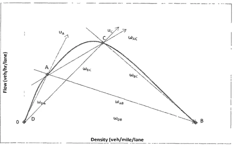
2.1.2 Shockwave analysis at signalized intersections
Queue length (horizontal queue) at signalized intersections can be estimated using
Shockwave theory if a flow-density relationship and the traffic states of the queue are
specified. A typical flow- density curve is shown in Figure 2-2(a) and a distance - time
diagram is shown in Figure 2-2(b). During time to to tj, the signal is green and traffic
proceeds and the traffic state A is represented by flow (qA)and density (kA). At time ti,
the traffic signal changes to red and traffic state immediately upstream of the stop line
changes to the traffic state B while the traffic state immediately downstream changes to
state D. Three shock waves begin at time t] at the stop line. These are a>AD, <*>DB anc* W
AB-When the departure flow at the stop line increases from zero to saturation flow the
traffic state C forms. This terminates Shockwave CODB and generates two new Shockwaves,
CODC and COBC- The flow states of A, B, C and D continue until coAB and coBc intercept at
time t3. At time tj a new Shockwave ooAc is formed, and the two Shockwaves COAB and OOBC
J S HI
o
Density |veh/m|fe/lane
(a) flow- density relationship
FJT7T7
/ r-s/
®
x^Dc <• oyA'Ss**,,.
'/
©*'
V / / / /WA B /
m////
//
7^f///9.
/ / / / / / / / / / / / / ' / . ' / / / / / / / / . / . /
/ w
®
I I I
t5 t .
Time
(b) Distance - time diagram
Based on this shock wave theory, a number of real-time estimation of
vehicle-count and queue length estimation models were recently developed (Strong et al., 2006;
Sharma et al., 2007; Skabardonis and Geroliminis, 2008; Vigos et al., 2008; Liu et al.,
2009; Zheng et al., 2009; Ban et al., 2010).
2.2 Real-time queue length estimation model
2.2.1 Input-Output and Hybrid queue length estimation technique
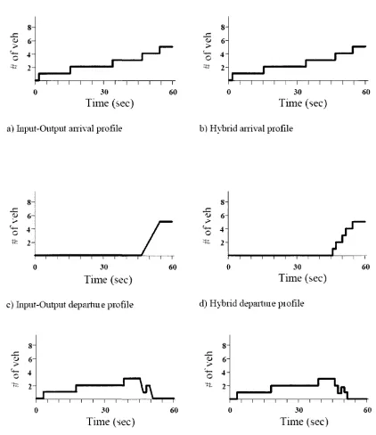
Sharma et al. (2007) applied two techniques (Input-Output and Hybrid technique)
for the real time prediction of vehicle delay and queue length at signalized intersections
based on the cumulative arrival and departure traffic counts collected from loop
detectors. The Input-Output technique uses advance detector actuations, signal timing
data and parametric data (e.g. saturation headway, start-up lost time, arrival shift, storage
capacity etc). In case of Input-Output technique, advance detector is placed upstream of
the stop line for recording arrival flow over time (input). On the other hand, the estimated
saturation flow rate is used to determine the number of vehicles crossing the stop line
over time (output). These two flow profiles are used to calculate the number of vehicles
in a queue approach between stop line and the location of the advance detectors (Sharma
et al., 2007).
The Hybrid technique uses advance detector actuations, stop bar detector
actuations, phase change data and parametric data (e.g. storage capacity etc) as model
inputs. The Hybrid technique records number of vehicles passing the loop detectors
placed upstream of the stop line for counting arrival flow and at the stop bar for counting
departure flow. The number of vehicle in a queue is calculated using arrival and
multiplying the number of vehicle in a queue by the effective length of vehicles in jam
traffic state. However, the evolution report showed that the result for the Hybrid
technique was not as good as the Input-Output technique in spite of using more input data.
The graphical representation of the Input-Output and Hybrid technique are shown in
Figure 2-3.
However, there were some limitations with this method: (i) "The Input-Output
method is insufficient for obtaining the spatial distribution of queue lengths in time"
(Michalopoulos and Stephanopolos, 1981); (ii) it cannot estimate queue length when a
queue spills over the location of detector (Liu et al., 2009); (iii) both the Input-Output and
Hybrid techniques were developed based on the assumption that vehicles do not change
lanes after they cross the advance detectors might degrade the performance of the
technique and (iv) the Input-Output method used many assumed values of input
parameters (e.g. saturation flow rate, storage capacity, etc).
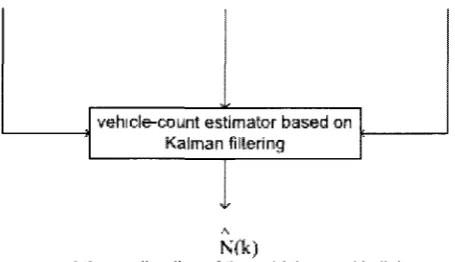
Vigos et al. (2008) developed a methodology for real-time estimation of
vehicle-count within signalized links. The number of vehicles in signalized links is valuable
information for urban signal control. A Kalman-Filter was used to estimate vehicle
counts in real time in signalized links based on measurements at (at least) three loop
detectors stations located at both end points and the middle of the link. The vehicle-count
estimation problem is illustrated in Figure 2-4. Figure 2-4(a) depicts the relevant signal
and detector configuration on the signalized link. The upstream signal (if it exists)
determines the traffic demands approaching the link while the downstream signal
8-yj 6"
o * 2
-J
J"~ i — i — i — i — i — i — i — i — r 0 30
Time (sec)
a) Input-Output arrival profile
" i — r 60
8
>
* 2-\
J
i i i r i i i i
30
Time (sec)
n — r 60
b) Hybrid anival profile
8
>
tfc
2-l I I I I I I I I 2-l 1 1—r
0 30 60
Time (sec)
c) Input-Output deparhue profile
8-1» 6
o 4 te. 2
-i -i r I I I I 1 — i — i r / :
30 60
Time (sec)
d) Hybrid deparhue piofile
8
r-1= 2H
" i I I I I I I I r
0 30
Time (sec)
60
e) Input-Output queue profile for computing delav
8
"3 6"
o n
"* 21
r
^ \ i — i — i — i — i — i — i — i — i — r
30 60
Time (sec)
f) Hybiid queue profile for computing delay
Obviously, whenever the link demand is larger than the link outflow, a queue is
built. It is shown in Figure 2-4(a) that three detectors are installed: at the upstream end of
the link, at the downstream end of the link and in the middle of the
Both boundary detectors provide flow measurements, while the middle detector
provides time-occupancy measurements. The basic structure of the queue estimation is
shown in Figure 2-4(b). The estimator is imported in real-time (every k) with the flow
and time-occupancy measurements from the link detectors. The estimators produce the
estimated number of vehicles in the link (between the two boundary detectors) for every
k. The number of vehicles in a link obeys the following conservation equation:
N (k) = N (k-1) + [qin (k-1) - qout (k-1)] (2-1)
where N(k) denotes the number of vehicles in the link at time k and k is the sampling
time (e.g. 20 sec); qin (k-1) and qout (k-1) are the flows entering and exiting, respectively,
the link during the period [(k-1), k].
2.2.2 Shockwave maximum queue length estimation techniques
Liu et al. (2009) developed a method to estimate the real-time queue length for
the congested signalized intersection using the Shockwave theory. They used the
SMART-SIGNAL (Systematic Monitoring of Arterial Road Traffic and Signals) data
collected from the advance detector placed upstream of the stop line. This method
enables the estimation of queue length even when a long queue spills over the advance
< • • !
link inflow time-occapancy
measurements q J (k -1) measurerrteats •£; f k -1}
link outflow
(a) The signal and detector configuration on the link
vehicle-count estimator based on Kalman filtering
real-time estimation of fhe vahicle-ceunt in link
(b) The link vehicle-count estimation
FIGURE 2-4: Vehicle-count estimation (Vigos et al., 2007)
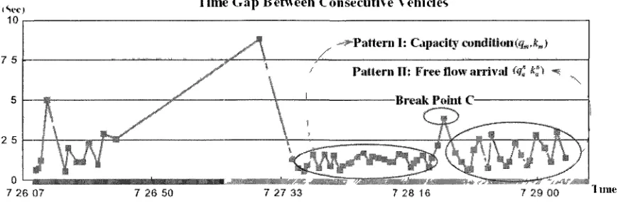
The high-resolution event-based data collected by the SMART-SIGNAL identify
"Break Points" (A, B, and C) in the occupancy profile and time gap profiles which
indicate the times when the traffic condition changes within a cycle (Figure 2-5 & 2-6).
These break points are used to calculate the speed of different Shockwaves
generated at the signalized intersection due to signal changes. The Shockwave
iSet) Detector f Jccupancv Time
7 28 50
V2S
7 27 33
FIGURE 2-5: Detector occupancy profile in a cycle (Liu et al., 2009)
1
Time Gap Between Consecutive Vehicles
7 5
^X
"-Pattern I: Capacity eoaditkmig^,^)
Pattern ITs Free flow arrival <•€ K^ «$
Break Ptmit
C-f-~S
2 5
7 28 16 7 29 00 l i m e
Loop r Detector m-J
Time
Red Green Red
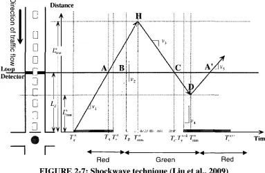
FIGURE 2-7: Shockwave technique (Liu et al., 2009)
When the signal turns to red (Tgn), two shock waves are generated. First, a queuing
Shockwave propagates toward the upstream of the traffic flow at a speed vi. At the start
of the green time (Trn), the queue begins to discharge at saturation flow state and a
discharge Shockwave propagates towards the upstream of the flow at a speed V2. When vi
and V2 meet a Tn max, a departure Shockwave propagates toward the stop line at a speed v3.
For over-saturation condition, the queue cannot be fully discharged within one cycle and
the fourth shockwave is formed to generate a residual queue moving upstream at a speed
v4.
Once Break Points (A, B, and C) have been identified, the flow (q) and density (k)
of each traffic state (i.e. the arrival traffic state (qa, ka) and saturation traffic state (qm, km))
can be calculated based on detector occupancy times and time gaps between vehicles.
The wave speed of v3 can be estimated using following equation (Liu et al., 2009):
The discharge wave speed V2 can be calculated based on the distance from the
stop bar (Ld), the difference between the green start time (Tr) and the time when the
discharge wave reaches advance detector (TB) as shown in the following equation (Liu et
al., 2009):
v 2 = - ^ r (2-3)
where, Lj is the distance from the stop line to the loop detector and TB is the moment
when the discharge Shockwave (V2) passes the detector at point B.
Liu et al. (2009) also developed the following equation to calculate the maximum
queue (Lmax) using the estimated values of v2 and v3 (Figure 2-6):
^max = ^d +~T~ 7~T (2-4)
vv2 v3 y
where TA is the moment when the queuing Shockwave (vi) passes the detector at point
A and Tc is the moment when the departure Shockwave (v3) passes the detector at point
C.
However, the method cannot estimate the queue length when oversaturation
occurs. Also, the Break Point C cannot always be determined because two traffic states
(queue discharge flow and new arrival flow) are not easily distinguished. Only one type
of vehicle (car) is considered in this method. Since this method uses a pre-determined
constant effective vehicle length of 7.62 m (25 ft) to estimate individual vehicle speed, it
Skabardonis and Geroliminis (2008) proposed an analytical kinematic wave
model to construct a link travel time and queue length estimate using aggregated
30-second flow and occupancy data from a loop detector upstream of the stop line and the
exact times of the red and green phases from the signal controller, the researchers used
the aggregated 20-30 second average data.
The arrivals at the upstream detector at distance Ld from the stop line can be
predicted as follows: If the flow is near zero, the queue exists. If the sufficiently low flow
follows the saturation flow, the queue clears and new flow arrives. As vehicles are
moving at free flow speed when departing from the queue, the traffic state changes from
the jam state to the saturation state. The maximum length of queue can be identified using
data from a detector placed at distance (Ld) upstream of the stop line and the geometry of
trapezium (ABCD) in Figure 2- 8 (Skabardonis and Geroliminis, 2008)
Lm = [u f • w / (u f + w)] • g + Ld = (c / k j) • g + Ld (2-5)
where, Lm = maximum length of queue; c = cycle length; g = green phase; kj = jam
density; Uf = free flow speed in the absence of queues; and w = congested shock wave.
However, free flow speed (uf) is not always constant in different traffic
conditions, and it leads to error in estimation. Since 30-s aggregation dampens variations
in vehicle gaps, it is difficult to identify the end of the queue unless the arrival traffic
flow is significantly lower than the queue discharge flow. Since queue length estimation
was only part of their travel time estimation model, the accuracy of the queue length
distance
« -
M
K \
A stop line
\ . \
\ L4 I \ \ \\w \ w \
\ \ ti \fe ; h\ \ \
"• - - ^- ^#^\^zt^%^u^u^, d etecto r
FIGURE 2-8: Space-time diagram (Skabardonis and Geroliminis, 2008)
2.2.3 Recent queue length estimation method
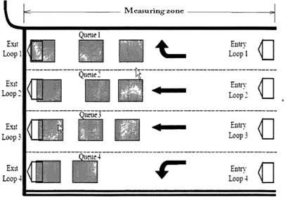
Zheng et al. (2009) developed algorithms designed for measuring average control
delay and queue length (vertical queue) at signalized intersections using traffic count data
collected from Video Image Processors (VIPs). These algorithms are implemented in a
computerized system called In-PerforM (Intersection Performance Measurement) for
measuring the performance of signalized intersections in real time. In this study, all the
lanes of the approach are equipped with two traffic sensors, placed upstream of the stop
line and at the stop line as shown in Figure 2-9. The area between the entry loop and exit
loop is called the measuring zone. The difference in the vehicle counts between the entry
loop and the exit loop (i.e. vehicles inside the measuring zone) in each lane is taken as the
This study estimated lane-by-lane queue length (vertical queue) considering the
lane flow, and the left-turn and right-turn flow ratios. This study estimated lane-by-lane
queue length (vertical queue) using vehicle counts in each lane obtained from detectors
upstream of the stop line and at the stop line.
M easuring z o n e
Exit Loopl
Exit Loop!
Exit Loop 3
Exit
Loop 4
/m
Queue 1
Entry
Loop I
n
Queue 2
i"
Entry / Loop I T
<
irtry y E:
Lsop3
>.*v.f4
01
EfltTA'Loop 4
FIGURE 2-9: Layout and sensor configuration of the study site (Zheng et al., 2009)
In spite of considering lane-specific queue length, the method implicitly assumes
that vehicles do not change lanes as they pass the detectors upstream of the stop line. If
more vehicles change lanes after passing the detectors, the estimated queue length is
Similar to the Input-Output method, this method cannot estimate the queue length
if the vehicle queue extends beyond the entry loop. Lane change activity within
measuring zone was not taken into consideration. This study assumes the constant vehicle
length of 5.5 m (18 ft).
Ban and Hao (2010) recently developed a new method to estimate queue length at
signalized intersections using sampled travel times of individual vehicles. Sampled travel
times are directly measured using the GPS equipped mobile traffic sensors within Virtual
Trip Lines (VTL). VTL is referred to as the upstream and downstream locations of an
intersection for travel time collection. The key concept of this method is the Queue Fully
Discharge Time (QFDT), which is the time when the queue would have been fully
discharged if there had been enough green time (Ban and Hao, 2010). This QFDT
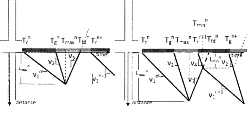
concept is based on Shockwave theory. Figure 2-10 depict the propagation of Shockwaves
in undersaturated and over-saturated condition respectively at a signalized intersection.
Trn and Tgn indicates the end and start time of the effective green during the nth cycle.
(a) Undersaturated condition (b) Oversaturated condition
The Queue Fully Discharge Time (QFDT) is defined as Tfdin Figure 2-10(a) and
2-10(b). For unsaturated conditions, QFDT is the time when the departure Shockwave (v3)
reaches the stop line, (i.e. the time that the queue is fully discharged). For over-saturation
conditions, Shockwave v3 meets residual Shockwave (v4) before it reaches the stop line, so
vehicles in the residual queue have to wait for an extra red time. Based on the definition
of QFDT, all of the queuing vehicles could be fully discharged from Tgn to Tfdn at a
saturation flow rate (qm). Therefore the maximum queue length of the n"" cycle is
Qnmax = ( Tn f d- Tn g) qm (2-6)
Similarly, the minimum queue length is
Qnmin = ( Tn f d- Tn + 1 r) qm (2-7)
However, mobile sensor data are only collected from the sample vehicles. They
do not represent the involvement of entire vehicles in a traffic stream. This study assumes
that arrival flow is uniform and the queue does not spill over the upstream VTL. Also, the
assumption that a queue clears in two cycles may not be valid in many arterial
intersections where the queue comprises long vehicles. Furthermore, lane changes
activity within the area between virtual trips lines are not taken into consideration in this
study.
2.3 Optimal location of detectors
Traffic data collected from loop detectors vary at different detector locations
upstream of the stop line at signalized intersections. In particular, the likelihood of queue
spillback and lane change is affected by the location of detectors. For instance, if loop
the detectors. Thus, lane-specific queue length estimation is more likely to be accurate.
On the other hand, queue spillback is more likely to occur and it is harder to estimate the
number of queued vehicles beyond the detector location. Thus, detector locations
significantly affect the accuracy of queue length estimation.
The past empirical studies reported that detectors were located at various
locations - 30-123 m (100-405 ft) upstream of stop line (Sharma et al., 2007; Liu et al.,
2009; Federal Highway Administration, 2006; Smaglik et al., 2007; Wang and Wu, 2007)
as shown in Table 2-1.
TABLE 2-1: Detector Location in Several Projects
Study
Wang and Wu, 2007
Liang ,2006
Oh and Choi, 2004
Federal Highway Admin., 2006
Project
Google Map based online platform for arterial traveler information (GATI) broadcast and analysis
Development of the real time arterial traffic flow map
Optimal detector location for estimating link travel speed in urban arterial roads
Traffic detector handbook: Third edition- volume 1, chapter 4,operations and intelligent transportation systems research
Distance from stop line
30 m - 40m
30 m - 42m
61m
61m
Location
Collected volume and occupancy data via loop detection placed at 30-40 m (100-130ft) in advance of intersection stop bars. City of Bellevue, Washington
Used advance loop detectors to collect volume and occupancy information placed approximately 30-42 m (100-140 ft) in advance of signalized intersections. City of Bellevue, Washington For links approximately 2000 ft in their lengths, the optimal detector location were identified to be about 61 m (200 ft) from
downstream intersection for green times of 20, 30,40 and 50
seconds, respectively. University Avenue, Madison Where a major driveway is located within a link, the loop should be located at least 15m (50 ft) downstream from the
TABLE 2-1: Detector Location in Several Projects (Continued)
Study
Gerolminis, 2009
Liu et al., 2009
Sharma et al., 2007
Smaglik et al., 2007
Thomas, 1998
Project
Queue spillovers in city street networks with
signal-controlled intersections
Real-time queue length estimation for congested signalized intersections Input-Output and Hybrid techniques for real-time prediction of delay and maximum queue length at signalized intersections Event-based data collection for generating actuated controller
performance measures Simulation of detector locations on an arterial street management system
Distance from stop line
75m
122m
123m
123m
91m, 183m, 274m
Location
System loop detectors are located on each lane approximately 75 m (250 ft) upstream of the
intersection stop line.
Lincoln Avenue, Los Angeles international Airport
Collected the data from the advance
detector placed at 122 m (400 ft) away from the stop line.
Rhode Ave., Minnesota
Collected data for arrival profile from the detector e placed at a distance 123 m (405 ft) in advance of the stop line. Noblesville, Indiana
Placed set-back detectors 123 m (405 ft) back from the stop bar at the northbound and southbound approaches at the INDOT intersection test bed. Noblesville, Indiana Varying the location of the downstream detector did not have a big impact on the output variables when the distance was greater than 122m (400 ft.). If detectors are placed less than 122m, the results could be misleading because vehicles are still accelerating close to the intersection.
Southern Avenue, Arizona
Although the location of detectors is important for capturing shock waves at
signalized intersections (Abbas and Bullock, 2003), no studies analyzed the impact of
detector location on queue length estimation and identified the optimal (or near optimal)
Given that the accuracy of the estimated queue length by the most real-time
models depends on the location of detectors, the determination of optimal location for
accurate queue length estimation is important. Some studies have examined
determination of the detector location for freeways and urban arterials.
Thomas (1998) derived the relationship between detector location and travel
characteristics (link speed, travel time, intersection delay) on arterial streets. The study
examined the relationship between traffic characteristics and detector locations for 92 m
(300 ft), 183 m (600 ft) and 275 m (900 ft) from the downstream intersection and 183 m
(600 ft) from the upstream intersection (Figure 2-11). Regression analysis was used to
evaluate the relationship between detector output values (occupancy and speed) and link
travel characteristics (link speed, travel time, intersection delay).
• • •
3 0 0 * <soo
O i r e c t i o n o t T r a v e l
•
D i r e c t i o n o r T r a v e l •
9(«) • •
1 <->oo •
! I O O
The study found that it is generally difficult to find "optimal" detector locations,
for all links in all cases. Although the results shows that 92 m (300 ft) point from the
downstream intersection was the optimal detector location^ it is valid only for existing
traffic volumes, green time, intersection geometric, lanes, and speed limit. Therefore, the
results might not be transferable to different sites and/or areas.
Thomas et al. (2000) have done a similar study in the same area. They used
CORSIM simulation in their research. CORSIM is a combination of microscopic network
simulation and microscopic freeway simulation model. CORSIM stimulates the
movement of individual vehicles by category in every second (Mystkowski and Sarosh,
1998). They found that varying the location of the downstream detector did not have a
significant impact on the output variables (volume, occupancy, speed) when the distance
was greater than 122 m (400 ft) from the downstream intersection. If the distance is less
than 122 m, the results could be misleading because vehicles are still accelerating close to
the intersection. They also found that there was no particular detector location with
higher accuracy of travel time than the other detector locations. The research showed that
detector data obtained on one link could not accurately predict link travel characteristics
on an adjacent link.
Oh and Choi (2004) developed an extended model based upon the research by
Sisiopiku et al. (1994) to find the optimal detector location using link travel speed in
urban arterial roads. They used the CORSIM traffic simulation with changing link length,
traffic volume, average link speed, detector location, number of lanes and estimated the
that the link average speed is similar to the speed measured at the detector (Oh and Choi,
2004).
It was found that the optimal detector location is determined by link length and
green time with other factors (number of lanes, traffic volumes, and speed limits) also.
The result shows that for links with approximately 610m (2000 ft), the optimal detector
locations were about 61m (200 ft) from downstream intersection for diverse green times
of 20 to 50 seconds. It was also found that with the increase of link length, optimal
locations were more dependent on green times. Figure 12 shows the results of optimal
detector locations.
*•"«. • M c
a
u
_o
o
4-»
u
I t
"O
15
O 2 5 0 "
/—v
-*rf C H 2 0 0 ^
_C
a 1 5 0 ® «
s
100 J2
u
5 0 | >
5
a
FIGURE 2-12: Optimal detector location (Oh and Choi, 2004)
The research focused on the detector locations over medium size links of 610 m
-2134 m (2000-7000 ft) in length. This limits the applicability of the results obtained in
this research if links which length is shorten than 610 m (2000 ft.) This research did not
include the issues of access, turning movement; effect of pedestrian's movement,
geometric components such as slope and lane width variations. Optimal Detector Locat
2000 4000 6000
Link Length from downstream interseetion(ft)
SQ00
20 seconds
BOscLwndi.
«—• 40i.ULOiidii
Abbas and Bullock (2003) developed a model to determine the location of
detector that can best capture the effect of Shockwaves formed at signalized intersection.
It was found that when the detector is placed very far from a signalized intersection, it
would not capture the existence of the Shockwave caused by the downstream bad offset.
On the contrary, if the detector was very close to the intersection, it would be affected by
the weaker Shockwave generated by the traffic turning from the side street.
Edara et al. (2008) developed a methodology to identify the optimal locations of
detectors on freeways in order to minimize the error in travel time estimation. They found
that the placement of detectors for estimating accurate travel time will vary by location
based on specific traffic and geometric conditions. They recommended that since the
traffic conditions change over time, detector placement will require periodic validation
and modification to ensure continued accuracy. The method showed that the detector
density needs to be higher in congested areas of corridor. Uncongested sections of the
corridor need only a nominal deployment.
An objective function is used to minimize the travel time estimation error.
Estimation error is the difference between the estimated travel time and the ground truth
travel time for the freeway section. The freeway section was divided into discrete
segments. This means that the detectors can be deployed only at the mid points of these
discrete segments. If there are m discrete locations then n detectors can be placed in mcn
possible ways (e.g. if m is 50 and n is 5, then the size of the solution space will be 50C5 =2
million combinations) (Edara et al., 2008). Exact solutions to such combinatorial
optimization problems were complex and not straight forward. A heuristic search
optimization using a population (set) of solutions (Goldberg, 1989). Steps involved in GA
are as follows (Edara et al., 2008):
(1) The parameter set for the problem has to be encoding first, as a binary or real number
representation.
(2) The initial population of P solutions (strings) has to be generating randomly and the
fitness value (objective function value) for each of these solutions has to be evaluated.
(3) Two strings from the current generation (parents) have to be selected for participating
reproduction, the selection probability being proportional to the fitness value.
(4) Parents selected in step 3 are mated by exchanging genetic material to produce two
offspring.
(5) Mutation operator is applied to the newly born offspring.
(6) Steps 3, 4 and 5 have to be repeated until offspring are generated. These offspring
constitute the new generation of solutions.
(7) The old population of solutions will have to be replaced with the newly generated
offspring and steps 3 through 7 will have to be repeated until a pre-specified number
of generations or other convergence criteria are met. Final solution is the best solution
from those discovered during the search.
However, this method is developed for a freeway with long distance to minimize the
error in travel time estimation. Thus, it may not be suitable for identifying the location of
CHAPTER III DATA
3.1 Study area
This study analyzes the signalized intersection at Huron Church Road and
Tecumseh Road in Windsor, Ontario, Canada as shown in Figure 3-1. The intersection is
one of the busiest intersections in Windsor due to its proximity to the Ambassador
Bridge, the busiest Canada-U.S. international border crossing. This intersection was
chosen since high volume of trucks pass through the intersection and a long queue of
vehicles frequently occurs on the northbound road. The posted speed limit at this
intersection is 60 km/h and the cycle length is 120 sec. The durations of displayed green
and red intervals for northbound through approach are 42 seconds and 71 seconds,
respectively.
Huron Church Road
12^ m
v h v --h h
-
•+-Stop Line
. - 5 6 , r n . h h
-:
Y—Y
Lane_3; Lan_e_2 ;
Lane 1 •
vay Driveway
165 m
Driveway
61 r 30 m
i
North
CD O
c 3 (A
CD 3 "
DO O
0)
a
Huron Church Road has three through lanes (Lanes 1, 2 and 3), an exclusive
left-turn lane and an exclusive right-left-turn lane. There are three driveways at 30 m, 61 m, and
165 m upstream of the stop line. To better understand the existing traffic conditions, data
were collected from this intersection during several weekdays of May, June and July
2009. Northbound traffic counts by vehicle type (car or truck), individual vehicle's length
and distance headway, queue length, and lane change frequency were observed in each
lane for each cycle.
3.2 Data collection
Data were collected during several days in May, June and July 2009 at the Huron
Church-Tecumseh intersection. Northbound traffic counts (left turn, through and right
turn) by vehicle type (car or truck) were collected in each lane, each phase and each
cycle. Signal timing, vehicle gap, distance headway (spacing), queue length, queue
spillback and mid-block traffic activities, e.g. lane changes, side encroachments, etc.
To observe the representative peak traffic volume, a long queue length and a high
percentage of trucks, data were collected from 11:00 am-12:00 pm and 3:30 pm-4:30 pm
in the weekdays. Data were collected under normal weather and daylight conditions.
To measure the vehicles length, gap (distance headway) between the vehicles and
the queue length, a scale was drawn on the sidewalk of the intersection with marks every
1.52 m (5 ft) from the stop line. The observer counted the number and type of vehicles
passing the intersection in each lane during the green interval and the number and type of
At the same time the observer also measured the length of the maximum queue
formed within the cycle using the marked scale on the sidewalk. The observer recorded
the time when the maximum queue was formed within the cycle using a stop watch. A
sample data sheet is enclosed in Appendix A-l.
3.2.1 Traffic counts
Only two types of vehicles, car and truck were observed in queue but other types
of vehicles (e.g. school bus, motor cycle) were not observed in queue during the data
collection periods at the intersection. The observed length of car at the intersection were
3.65 m, 4.26 m, 4.57 m, 4.87 m, 5.48 m and the observed length of trucks are 16.76 m,
21.34 m and 21.95 m. It was observed that the total volume was almost the same from 11
am12 pm and 3:30 pm 4:30 pm but the percentage of trucks was higher from 11 am
-12 pm in northbound traffic. Table 3-1 and Table 3-2 show the numbers of northbound
cars and trucks in each lane of Huron Church Road for 30 cycles during 11 am-12 pm
and 3:30 pm - 4:30 pm on June 5, 2009. A majority of trucks (78-83%) used the center
through lane (Lane 2). Due to high percentage of trucks in Lane 2 (45-56%), queue
length was longest in Lane 2 for most cycles. The percentage of trucks during this study
period was 13.5-16% and about two-third of total vehicles were through vehicles in
northbound traffic. Similar distributions of vehicles across lanes were also observed on
Table 3-1: Summary of Traffic Counts (11 am-12 pm, June 5, 2009) Total arrival (%) Total No. of stopped vehicles on red No. of passing vehicles on green Total Total C 740 (84) T 145 (16) 885
183 17
200
557 128
685 Left-turn Lane C 44 (96) T 2 (4) 46(6%)
38 2
40
6 0
6 Lane 3 (Through) C 210 (97) T 7 (3) 217 (24%) Lane 2 (Through) C 90 (44) T 114 (56) 204 (23%) Lane 1 (Through) C 208 (95) T 11 (5) 219 (25%) Car - 508 (79%) Truck- 132 (21%)
640 (72 %)
25 0
25
185 7
192
12 12
24
78 102
180
57
57
151 11
162 Right-turn Lane C 188 (95) T 11 (5) 199 (22%)
51 3
54
137 8
145 Note: C = Car; T = Truck
Table 3-2: Summary of Traffic Counts (3:30 pm-4:30 pm, June 5, 2009)
Total arrival (%) Total No. of stopped vehicles on red No. of passing vehicles on green Total Total C 768 (85) T 120 (13.5) 888
208 19
227
560 101
661 Left-turn Lane C 35 (100) T 0 (0) 35(4%)
29 0
29
6 0
6 Lane 3 (Through) C 245 (99) T 3 (1) 248 (28%) Lane 2 (Through) C 121 (55) T 100 (45) 221 (25%) Lane 1 (Through) C 180 (95) T 9 (5) 189 (21%)
Car - 546 (83%) Truck- 112 (17%)
658 (74 %)
37 0
37
208 3
211
26 15
41
95 85
180
53 3
56
127 6
133 Right-turn Lane C 187 (96) T 8 (4) 195 (22%)
63 1
64
124 7
Since the traffic data were manually collected at the intersection, there were
some possible errors associated with counting the number of queued vehicles, measuring
the length of vehicles, the length of queue, and gap between the queued vehicles.
3.2.2 Lane change
The number of lane changes was also observed at two areas - the areas within
56 m (184 ft) and 122 m (400 ft) in advance of the stop line during the study period as
shown in Table 3-3.The count of number of lane changes could be easily done manually
in the field and there were a possibility of miscounting the number of lane changes but
the total impact of such error was insignificant in our collected data. Within the area of
56 m and 122 m from the stop line, on average 30 and 74 lane changes (excluding lane
changes by the vehicles entering or exiting the driveways) respectively occurred during
different one-hour periods on different weekdays. This indicates that after vehicles pass
the location closer to the stop line, they are less likely to change lanes.
TABLE 3-3: Number of Lane Changes
Distance from stop-line
56 m 56 m 122 m 122 m
Date
July 17, 2009 July 21, 2009 July 17, 2009 July 21, 2009
Time
5:00 pm - 6:00 pm 12:30 pm-1:30 pm 4:00 pm-5:00 pm 1:30 pm-2:30 pm
Phase
Red+ Green Red+ Green Red+ Green Red+ Green
No. of lane changes
59 41 119 108
3.2.3 Mid-block driveways
There are two driveways for vehicles to enter or leave from the gas station located
at the southeastern corner of Huron Church-Tecumseh intersection. The driveways are 30
(45 ft) and 15 m (50 ft). Another driveway to the American Plaza is located 165 m (540
ft) from the stop line as shown in Figure 3-1.Table 3-4 shows the total number of vehicles
entering and exiting from the driveways at two locations 56 m and 122 m from the stop
line.
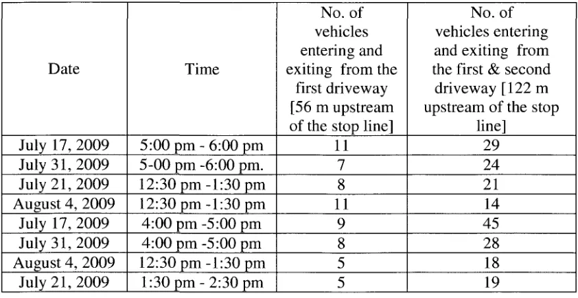
Table 3-4: Number of Vehicles Entering and Exiting Driveway
Date
July 17, 2009 July 31, 2009 July 21, 2009 August 4, 2009
July 17, 2009 July 31, 2009 August 4, 2009
July 21, 2009
Time
5:00 pm-6:00 pm 5-00 pm -6:00 pm. 12:30 pm-1:30 pm 12:30 pm-1:30 pm 4:00 pm -5:00 pm 4:00 pm -5:00 pm 12:30 pm-1:30 pm
1:30 pm-2:30 pm
No. of vehicles entering and exiting from the
first driveway [56 m upstream of the stop line]
11 7 8 11
9 8 5 5
No. of vehicles entering and exiting from the first & second
driveway [122 m upstream of the stop
line] 29 24 21 14 45 28 18 19
The number of vehicles entering and exiting the driveways was observed at two
observation points - 56 m (185 ft) and 122 m (400 ft) upstream of the stop line. At 56 m
from the stop line, the vehicles entering and exiting the driveway at 30 m from the stop
line could not be counted. However, these "missing" vehicles were only 1.1% of total
northbound vehicles. At 122 m from the stop line, the vehicles entering and exiting the
two driveways at 30 m and 61m from the stop line could not be counted. These missing
vehicles were only 2.8% of total northbound vehicles. Thus, the vehicles entering or
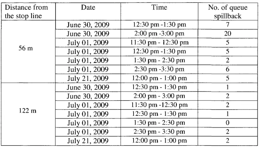
3.2.4 Queue spillback
It was observed that queue sometimes spills over the two potential locations of
detectors- 56 m and 122 m from the stop line. As expected queue spillback occurs more
frequently at 56 m from the stop line than 122 m from the stop line. Frequent queue
spillback makes difficult to detect the number of queued vehicles beyond the location of
detectors. Table 3-5 summarizes the results of field observation in each day.
It was observed that maximum queue length was longer than the distance between
the stop line and observation point for 7 out of 30 cycles at 56 m from the stop line and
1.4 out of 30 cycles at 122 m from the stop line. This indicates that if detectors are
located further away from the stop line, queue is less likely to pass detectors and the
number of vehicles beyond the detector location is lower. Clearly, for more accurate
estimation of queue length, detectors should be neither too close to the stop line (due to
frequent queue spillback) nor too distant from the stop line (due to frequent lane
changes).
3.2.5 Right-turn and left-turn lane
At the Huron Church-Tecumseh intersection, the right-turn lane with full width
(3.66m) starts 164m from the stop line and the left-turn lane with full width start 56m
from the stop line. If the location of data collection points is placed at or within 56 m it
would be possible to capture all the through, left-turn and right-turn vehicles. On the
other hand, if the data collection points are placed at 122m, left-turn vehicles cannot be
TABLE 3-5: Number of Queue Spillback
Distance from the stop line
56 m
122 m
Date
June 30, 2009 June 30, 2009 July 01, 2009 July 01, 2009 July 01, 2009 July 01, 2009 July 21, 2009 June 30, 2009 June 30, 2009 July 01, 2009 July 01, 2009 July 01, 2009 July 01, 2009 July 21, 2009
Time
12:30 pm-1:30 pm 2:00 pm -3:00 pm 11:30 pm-12:30 pm
12:30 pm-1:30 pm 1:30 pm-2:30 pm 2:30 pm -3:30 pm 12:00 pm- 1:00 pm 12:30 pm- 1:30 pm 2:00 pm - 3:00 pm 11:30 pm-12:30 pm
12:30 pm- 1:30 pm 1:30 pm- 2:30 pm 2:30 pm- 3:30 pm 12:00 pm-1:00 pm
No. of queue spillback
7 20
5 5 2 6 5 1 2 2 1 0 2 2
It is also observed in the study area that the length of both turning lanes is
sufficient to store all queued vehicle since these lanes are normally used by the short
vehicles (car).However, the long queue in lane 2 (which is generally created due to long
vehicles) sometimes prevents from entering the left-turn lane.
3.2.6 Length of vehicles, gap between vehicles and queue length
It was observed that the length of cars was 3.7-5.5 m (12-18 ft) and the length of
trucks was 16.8-21.9 m (55-72 ft). The average distance headway between vehicles was
different for different vehicle types. The headways for car following car, truck following
car, and truck following truck (car following truck was not observed during the study
period) were 3.7 m, 4.6 m and 5.7 m, respectively. This indicates that trucks tend to
longer length and headway of trucks, queue length longer when there are more trucks in a
queue.
TABLE 3-6: Observed Queue Length by Vehicle Type
Vehicles in a queue 3 cars 4 cars 2 trucks 3 trucks 4 trucks 5 trucks
Observed queue length (ft)
7 0 - 8 0 88 - 1 2 5 147 - 168
200- 269
310 - 365
390 - 445
Vehicles in a queue 1 truck + 2 cars 1 truck + 5 cars 2 trucks + 1 car 4 trucks + 1 car 5 trucks + 1 car
Observed queue length (ft)
135 215 200-205
385 470
3.2.7 Signal timing
The cycle length at the Huron Church-Tecumseh intersection is 120 seconds.
Displayed green intervals are shown in Table 3-7. Intergreen period (red + amber)
between phases are 3-4 sec. The effective green time is the time allocated for a given
traffic movement (green plus yellow) at a signalized intersection less the start-up and
clearance lost times for the movement (Kang, 2000). Highway Capacity Manual (2000)
states the effective green time is equal to the actual (displayed) green time plus the
change-and-clearance interval minus the lost time for the movement. The effective red
interval is cycle length minus the effective green interval. The effective green time and
effective red time were calculated using different parametric values available at the study
site in the following equation developed by Mannering et al. (2009):
g = G + Y+AR - tL (3-1)
where g = effective green time (seconds); G = displayed green time (seconds);