https://doi.org/10.5194/nhess-19-1685-2019 © Author(s) 2019. This work is distributed under the Creative Commons Attribution 4.0 License.
Statistical analysis for satellite-index-based insurance
to define damaged pasture thresholds
Juan José Martín-Sotoca1, Antonio Saa-Requejo2,3, Rubén Moratiel2,3, Nicolas Dalezios4, Ioannis Faraslis5, and Ana María Tarquis2,6
1Data Science Laboratory, European University, Madrid, Spain
2CEIGRAM, Research Centre for the Management of Agricultural and Environmental Risks, Madrid, Spain 3Department of Agricultural Production, Universidad Politécnica de Madrid, Madrid, Spain
4Department of Civil Engineering, University of Thessaly, Volos, Greece
5Department of Planning and Regional Development, University of Thessaly, Volos, Greece 6Complex Systems Group, Universidad Politécnica de Madrid, Madrid, Spain
Correspondence:Juan José Martín-Sotoca ([email protected]) Received: 7 February 2019 – Discussion started: 19 February 2019
Revised: 18 June 2019 – Accepted: 9 July 2019 – Published: 7 August 2019
Abstract. Vegetation indices based on satellite images, such as the normalized difference vegetation index (NDVI), have been used in countries like the USA, Canada and Spain for damaged pasture and forage insurance over the last few years. This type of agricultural insurance is called satellite-index-based insurance (SIBI). In SIBI, the occurrence of damage is defined as normal distributions. In this work a pasture area at the north of the Community of Madrid (Spain) has been delimited by means of Moderate Resolution Imaging Spectroradiometer (MODIS) images. A statistical analysis of NDVI histograms was applied to seek for alternative distributions using the maximum likelihood method and χ2 test. The results show that the normal distribution is not the optimal representation and the generalized extreme value (GEV) distribution presents a better fit through the year based on a quality estimator. A comparison between normal and GEV is shown with respect to the probability under a NDVI threshold value throughout the year. This suggests that an a priori distribution should not be selected and a percentile methodology should be used to define a NDVI damage threshold rather than the average and standard deviation, typically of normal distributions. Highlights.
– The GEV distribution provides better fit to the NDVI historical observations than the normal one.
– Differences between normal and GEV distributions are higher during spring and autumn, which are transition periods in the precipitation regimen.
– NDVI damage threshold shows evident differences us-ing normal and GEV distributions both coverus-ing the same probability (24.20 %).
– NDVI damage threshold values based on percentile cal-culation are proposed as an improvement in the index-based insurance in damaged pasture.
1 Introduction
insured smallholders, due to the fact that the risk of nonre-payment for lenders is reduced, which encourages the use of agricultural inputs and equipment, leading to increased and more stable crop production. Over the past decade, the importance of weather-index-based insurances (WIBIs) for agriculture has been increasing, mainly in developing coun-tries (Gommes and Kayitakire, 2013). This interest can be explained by the potential that IBI constitutes a risk man-agement instrument for small farmers. Indeed, it can be con-sidered within the context of renewed attention to agricul-tural development as one of the milestones of poverty reduc-tion and increased food security, as well as the accompany-ing efforts from various stakeholders to develop agricultural risk management instruments, including agricultural insur-ance products.
Farmers need to protect their land and crops specifically from drought in arid and semiarid countries, since their pro-duction may directly depend mainly on the impacts of this particular natural hazard. Insurance for drought-damaged lands and crops is currently the main instrument and tool that farmers can resort to in order to deal with agricultural pro-duction losses due to drought. Many of these insurances are using satellite vegetation indices (Rao, 2010); thus they are also called satellite-index-based insurances (SIBIs). SIBIs have some advantages over WIBIs, such as cost-effective information and acceptable spatial and temporal resolution. They do not, however, resolve the issue of basis risk, i.e., po-tential unfairness to insurance takers (Leblois, 2012). More-over, the very nature of an index-based product creates the chance that an insured party may not be paid when they suffer loss. For this reason, in some countries (Spain) they have named this SIBI “damaged in pasture” to cover not only drought even though this is the main cause.
It is highly recognized that shortage of water has many im-plications for agriculture, society, the economy and ecosys-tems. Specifically, its impact on water supply, crop produc-tion and rearing of livestock is substantial in agriculture. Knowing the likelihood of drought is essential for impact prevention (Dalezios, 2013). Drought severity assessment can be approached in different ways: through conventional indices based on meteorological data, such as temperature, rainfall and moisture (Niemeyer, 2008), as well as through remote sensing indices based on images usually taken by arti-ficial satellites (Lovejoy et al., 2008) or drones. In the second group, satellite vegetation indices (SVIs) are found, which can quantify green vegetation and soil moisture through the soil water index (Gouveia et al., 2009) combining different spectral reflectances. Thus, they are one of the main ways to quantitatively assess drought severity.
At the present time, several satellites (NOAA, TERRA, DEIMOS, etc.) can provide this spectral information with different spatial resolution. Some series with a high temporal frequency are freely available – those from NOAA satellites and Terra. The most widely known SVI is the normalized difference vegetation index (NDVI). It follows the principle
that healthy vegetation mainly reflects the near-infrared fre-quency band. There are several other important SVIs, such as the soil adjusted vegetation index (SAVI) and enhanced veg-etation index (EVI), that incorporate soil effects and atmo-spheric impacts, respectively. An important point of SIBI is when damage occurs. To measure this, a SVI threshold value is defined mainly based on statistics that apply to normal dis-tributed variables: average and standard deviation. When cur-rent SVI values are below this threshold value for a period of time, insurance recognizes that damage is occurring, most of the time drought, and then it begins to pay compensation to farmers.
Important NDVI-based indices for detecting drought are the NDVI anomalies (NDVIA) and standardized vegetation index (SVI). NDVIA and SVI have been successfully used to monitor drought conditions over different regions in the world (Nanzad et al., 2019; Li et al., 2014). NDVIA is cal-culated as the difference between the NDVI value for a specific time period (e.g., week, month) and the long-term mean value for that period. SVI was developed by Peters et al. (2002) and obtains the probability from normal NDVI dis-tributions over multiple years of data for a specific time pe-riod (Anyamba and Tucker, 2012; Bayarjargal et al., 2006). It is defined as
SVIi=
NDVIi−NDVI σNDVI
=NDVIAi
σNDVI
, (1)
where NDVI is the long-term mean NDVI in the periodi, σNDVIis the standard deviation of NDVI in the periodiand NDVIi is the current NDVI value in the time periodi. Using only the first and second statistical moment, the average and the square root of variance, the assumption of normality is implicit in this type of drought NDVI indicator. The normal-ity assumption is challenged in this study.
princi-ples of IBI, as otherwise the insurer, even the whole concept of insurance, is at risk of reputation loss for years or decades. There is currently a lack of technical capacity in the insur-ance sectors of most developing countries, which is a con-straint to the scaling up and further development of WIBI (Gommes and Kayitakire, 2013). Specifically, although it is possible to design an index product and assist in the roll-out, marketing and sales, such assistance is not possible on a wide scale, simply because there is a lack of qualified ex-pertise. Indeed, it usually requires mathematical modeling, data manipulation and expertise in crop simulation to design an index. Nevertheless, it is possible to structure insurance with multiple indices, but this increases the complexity of the product and makes it difficult for farmers to comprehend it. Basis risk is also a particular problem for index products, which is frequently caused by the fact that measurements of a particular variable, such as rain, may differ at the insurer’s measurement site and in the farmer’s field. This also creates problems for insurance providers. Indeed, part of the reason the scaling up of index products has failed is that both insur-ers and farminsur-ers suffer from this basis risk.
Currently, to mitigate impacts of climate-related reduced productivity of French grasslands, several studies have been developed to design new insurance-scheme-based indem-nity payouts to farmers on a forage production index (FPI) (Roumiguié et al., 2015, 2017). Two examples of SIBIs are presented in two different countries: the USA and Spain. In particular, in the USA there are several insurance pro-grams for pasture, rangeland and foraging, which use var-ious indexing systems (rainfall and vegetation indices) and are promoted by the Unites States Department of Agricul-ture (USDA) (Maples et al., 2016; USDA, 2018). NDVI is the index chosen in the vegetation index program, and it is obtained from the AVHRR (Advanced Very High Resolu-tion Radiometer) sensor aboard NOAA satellites. Average, maximum and minimum NDVI values are obtained from a historical series with the aim of calculating a trigger value. The insurer decides the quantity of compensation by com-paring this trigger with the current value. On the other hand, in Spain insurance for damaged pasture is available from the Spanish System of Agricultural Insurance (BOE, 2013). This insurance defines a damage event through NDVI val-ues obtained from the MODIS sensor aboard the TERRA satellite of NASA. In this insurance, NDVI threshold val-ues (NDVIth) are calculated by subtracting several times (k=0.7 ork=1.5) standard deviation to average within a homogeneous area:
NDVIth=µ−k·σ, (2)
where µ and σ are the average and standard deviation of NDVI respectively. The average and standard deviation are derived supposing normal distributions in the historical data (Goward et al., 1985; Hobbs, 1995; Fuller, 1998; Al-Bakri and Taylor, 2003; Turvey and Mclaurin, 2012; De Leeuw et al., 2014).
The aim of this paper is to find a more realistic statisti-cal NDVI distribution without the a priori assumption that variables follow a normal distribution, typically for current SIBI methodology. In order to achieve this, the maximum likelihood method (MLM) is fitted to a historical series of NDVI values in a pasture land area in Spain (Community of Madrid). Different types of asymmetrical distributions are examined with the aim to find a better fit than normal. To eliminate some noise in the historical series, an original method is applied consisting of using the hue–saturation– lightness (HSL) color model. Finally, the Chi-square test (χ2test) has been used to check the goodness of fit for all considered distributions.
2 Materials and methods 2.1 Vegetation index
The differences of the reflectance of green vegetation in parts of the electromagnetic radiation spectrum, namely visible and near infrared, provide an innovative method for moni-toring surface vegetation from space. Specifically, the spec-tral behavior of vegetation cover in the visible (0.4–0.7 mm) and near infrared (0.74–1.1, 1.3–2.5 mm) offers the possi-bility to monitor from space the changes in the different stages of cultivated and uncultivated plants taking also into account the corresponding behavior of the surrounding mi-croenvironment (Ortega-Farias et al., 2016). Indeed, from the visible part of the electromagnetic radiation spectrum it is possible to draw conclusions about the rate photosynthe-sis, whereas from the near infrared inferences are extracted about the chlorophyll density and the amount of canopy in the plant mass, as well as the water content in the leaves, which is also linked directly to the rate of transpiration with impacts to physiological process of photosynthesis. Usu-ally, data from the NOAA/AVHRR series of polar orbit me-teorological satellites are used with low spatial resolution (1.1 km2) and a recurrence interval at least twice daily from the same location. Several algorithms combining channels of the red (RED), the near infrared (NIR) and green (GREEN) have been proposed, which provide indices sensitive to green vegetation.
NDVI uses two frequency bands: red band (660 nm) and near-infrared band (860 nm). Absorption of red band is re-lated to photosynthetic activity and reflectance of near-infrared band is related to the presence of vegetation canopies (Flynn, 2006). In drought periods, NDVI values can reduce significantly; therefore many researchers have used this in-dex to measure drought events in recent years (Dalezios et al., 2014). To calculate NDVI we will use this mathematical formula:
NDVI=IR−R
where IR and R are reflectance values in the near-infrared band and red band, respectively. NDVI values below zero indicate no photosynthetic activity and are characteristic of areas with large accumulation of water, such as rivers, lakes or reservoirs. The higher the NDVI value is, the greater the photosynthetic activity and vegetation canopies are.
In this paper the NDVI is used, which is a widely known index with a multitude of applications over time. The NDVI is suited for monitoring of total vegetation, since it partly compensates for the changes in light conditions, land slope and field of view (Kundu et al., 2016). In addition, clouds, water and snow show higher reflectance in the visible than in the near infrared; thus, they have negative NDVI values. Indeed, bare and rocky terrain show vegetation index values close to zero. Moreover, the NDVI constitutes a measure of the degree of absorption by chlorophyll in the red band of the electromagnetic spectrum. In summary, the NDVI is a reli-able index of the chlorophyll density on the leaves, as well as the percentage of the leaf area density over land; thus, NDVI constitutes a credible measure for the assessment of dry mat-ter (biomass) in various species’ vegetation cover (Dalezios, 2013). It is clear from the above that the NDVI is an index closely related to growth and development of plants, which can effectively monitor surface vegetation from space.
The continuous increase in the NDVI value during the growing season reflects the vegetative and reproductive growth due to intense photosynthetic activity, as well as the satisfactory correlation with the final biomass production at the end of a growing period. On the other hand, the grad-ual decrease in the NDVI values signifies stress due to a lack of water or extremely high temperatures for the plants, lead-ing to a reduction of the photosynthetic rate and ultimately a qualitative and quantitative degradation of plants. NDVI values above zero indicate the existence of green vegetation (chlorophyll), or bare soil (values around zero), whereas val-ues below zero indicate the existence of water, snow, ice and clouds.
2.2 Database
The scientific research satellite Terra (EOS AM-1) has been chosen to provide necessary information to calculate NDVI in the study area. This satellite was launched into orbit by NASA on 18 December 1999. The MODIS sensor aboard this satellite collects information of different reflectance bands. MODIS information is organized by products. The product used in this study was MOD09A1 (LP DAAC, 2014). MOD09A1 incorporates seven frequency bands: band 1 (620–670 nm), band 2 (841–876 nm), band 3 (459–479 nm), band 4 (545–565 nm), band 5 (1230–1250 nm), band 6 (1628–1652 nm) and band 7 (2105–2155 nm). The bands used to calculate NDVI are band 1 for red frequency and band 2 for near-infrared frequency. MOD09A1 provides geo-referenced images with a pixel resolution of 500 m×500 m. Each MOD09A1 pixel contains the best possible L2G
obser-vation during an 8 d period as selected on the basis of high observation coverage, low view angle, the absence of clouds or cloud shadow, and aerosol loading.
The period of time selected in this study was from 2002 to 2017.
Daily data from a principal station of the meteorologi-cal network were utilized during the period studied (2002– 2017). Meteorological station is located in 40◦4104600N 3◦4505400W (elevation 1004 m a.s.l.), less than 2 km from the study area (AEMET, 2017).
2.3 Site description
Six pixels (500 m×500 m) are considered located in a pas-ture area at the north of the Community of Madrid (Spain) between the municipalities of Soto del Real and Colmenar Viejo. The study area is located between meridians 3◦4500000 and 3◦4700000W and parallels 40◦4200000 and 40◦4400000N approximately (see Fig. 1).
The annual mean temperature ranges during the study period from 12.7 to 13.8◦C, and annual mean precipita-tion ranges from 360 to 781 mm. The staprecipita-tions studied were identified as semiarid (annual ratio P /ET0 between 0.2 and 0.5) according to the global aridity index developed by the United Nations Convention to Combat Desertification (UNEP, 1997). According to the climatic classification of Köppen (Kottek et al., 2006), this area presents a continen-tal Mediterranean climate temperate with dry and temperate summer (type Csb). Temperature and precipitation of this site, based on 20 years, is presented in Table 1.
Due to high soil moisture conditions, ash is the dominant tree, forming large agroforestry systems (dehesas) that are used for pasture. These are ecosystems with high biodiver-sity.
2.4 HSL model
There is no doubt that NDVI time series from satellite sen-sors carry useful information, which can be used for char-acterizing seasonal dynamics of vegetation (Fensholt and Proud, 2012; Forkel et al., 2013). However, due to unfavor-able atmospheric conditions during the data acquisition, the NDVI time-series curve often contains noise (Motohka et al., 2011; Park, 2013). Although most of the NDVI data products are temporally composited through the maximum value com-positing (MVC) method (Holben, 1986) to retain relatively cloud-free data, residual noise still exists in the data, which will affect the accuracy of the NDVI value.
Figure 1.The study area is in the center of the Iberian Peninsula (Community of Madrid). RGB image of the 6-pixel area used for the case study is shown (© Google Earth and MODIS images).
Table 1.Monthly average of maximum temperature (Tmax), average temperature (Tavg), minimum temperature (Tmin) and precipitation (P).
Study period from 1997 to 2017.
Month Jan Feb Mar Apr May Jun Jul Aug Sep Oct Nov Dec Annual
Tmax(◦C) 7.1 9.3 12.7 15.4 19.5 24.6 28.6 28.1 23.7 16.8 11.1 7.4 17.0
Tavg(◦C) 3.6 4.8 7.7 10.1 13.7 18.4 22.0 21.7 17.9 12.3 7.1 4.1 12.0
Tmin(◦C) 0.0 0.3 2.6 4.8 7.8 12.1 15.4 15.3 12.0 7.8 3.0 0.8 6.8
P (mm) 67.2 50.0 38.5 62.2 62.3 30.2 18.9 16.4 34.2 79.3 86.2 82.6 627.9
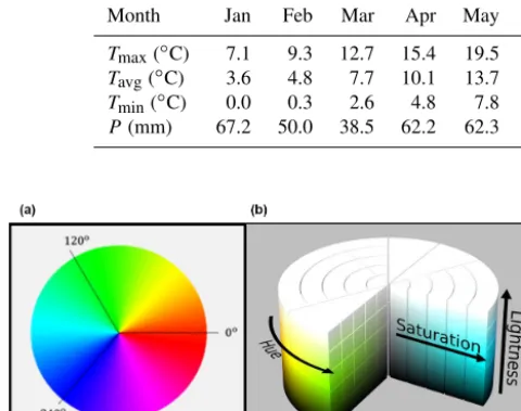
Figure 2. (a)Color wheel of hue.(b)The HSL model (Creative Commons).
lightness color model inspired by the work presented by Tackenberg (2007).
HSL color model is a cylindrical representation of RGB (red–green–blue) points. Their components are hue (color type), saturation (level of color purity) and lightness (color luminosity). Hue is the angular component, and it is more intuitive for humans since it is directly related to the color wheel (see Fig. 2).
Saturation is the radial component and near-zero values indicate gray colors. Lightness is the axial radial versus axial component, zero lightness produces black and full lightness produces white.
The NDVI series are filtered using the following HSL cri-terion: NDVI values are valid if HSL saturation is greater than 0.15. The pixels that have gray colors correlate well with pasture areas covered by clouds or snow. In these cases, the NDVI values calculated in these pixels are incorrect. Using the above HSL criterion, all these NDVI values are elimi-nated. This type of filter based in HSL color space has been used on digital camera images monitoring vegetation phe-nology (Tackenberg, 2007; Crimmins and Crimmins, 2008; Graham et al., 2009). However, we have not found the use of this HSL criterion in the context of NDVI remote sensing images.
2.5 Maximum likelihood method
L=f (x,θ)= n Y
i=1
f (xi; αβµσ, . . .), (4)
wherex=(x1, . . . ,xn)is the set of data,θ=(α,β,µ,σ, . . . ) is the vector of parameters andf (xi;αβµσ, . . . ) is the den-sity function of the statistical model.
When maximization with respect to the vector of parame-ters is carried out, the estimated parameparame-ters (α,ˆ β,ˆ µ,ˆ σˆ, . . . ) for the proposed statistical distribution are obtained (Larson, 1982). Important properties of these estimated parameters are consistency, efficiency and asymptotic normality.
In the case of a normal model, the estimated statistics µandσare defined by accurate expressions as follows:
ˆ
µ=x=1
n n X
i=1
xi σˆ =s= v u u t 1 n n X i=1
(xi−x)2, (5)
whereµˆ is the sample mean andσˆ is the sample standard deviation of the data set.
In this study we will apply MLM to estimate the parame-ters for four probability density functions (PDFs). In Table 2, a brief description is presented of these PDF candidates: nor-mal, gamma, beta and generalized extreme value (GEV). To do so, the following MATLAB functions have been used: normfit, gamfit, betafit and gevfit.
2.6 Goodness of fit (χ2test)
Theχ2test can be used to determine to what extent observed frequencies differ from frequencies expected for a specific statistical model. The most important points of the theory are briefly presented in Cochran (1952).
Let f (x, θ ) be a theoretical density function of a ran-dom variable X which depends on parameters θ=(α, β, µ,σ, . . . ) and let x1, . . . ,xn be a sample ofX grouped into kclasses withni data per classi.
Firstly, the following hypothesis is set: (H0) observed data fit theoretical distributionf (x,θ ).
Then the test statisticχc2is defined as
χc2= k X
i=0
(ni−ei)2 ei
, (6)
whereni is the number of data or observed frequency and ei=n·P(class i) is the expected frequency for class i. P(classi) is the theoretical interval probability defined for classi.
A level of significance is also set as
α=P (RejectH0/H0is true) . (7) Finally, the following decision rule is applied: reject the the-oretical distribution at significance levelαif
χc2> χ(k−m−1,1−α)2 , (8)
whereχ(k−m−1,1−α)2 is aχ2distribution withk−m−1 de-grees of freedom (mis the number of parameters,k is the number of classes).
3 Results
3.1 HSL filtering criterion
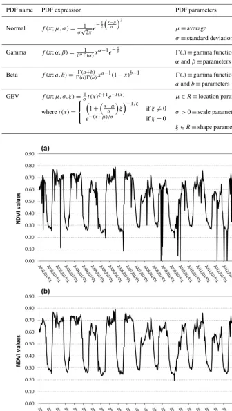
NDVI series (from 2002 to 2017) were obtained for each pixel of the study area using frequency bands provided by the MODIS product named MOD09A1. These series contain some irregular values that can skew the NDVI pattern. There-fore, the six series (6 pixels) were filtered using the HSL cri-terion.
MOD09A1 is a MODIS product that processes data to ob-tain the best observation in an 8 d period. However, it is pos-sible that the result of this selection still presents some prob-lems since the best selection is relative to the eight observa-tions of the period. For example, if the eight observaobserva-tions, at 1 pixel, appear with clouds, shadow clouds or snow, the best selection still shows this problem.
As an example of the above, the NDVI series (10 years) of 1 pixel of the study area is shown in Fig. 3. On the top graph of Fig. 3 there are extremely low NDVI values in some dates. If these NDVI values are compared to neighboring val-ues (8 d after or before) the high variation presented in such a short period is not plausible. This issue tells us that the MODIS sensor has not obtained a proper observation during this 8 d period (interval).
The HSL criterion helps us to eliminate these incorrect NDVI values, since the filter is interpreting that these pixels still contains clouds or snow, i.e., pixels with low saturation (grayish colors).
Figure 3 shows that abrupt changes in the NDVI values, mainly observed during raining seasons such as autumn and winter, are efficiently eliminated. Not being a highly compu-tationally demanding method is one of the main advantages of the HSL filtering method. Therefore, this method will al-low us to obtain more robust NDVI values to be used in the statistical analysis.
3.2 Statistical analysis
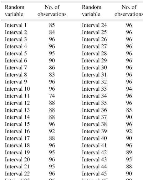
NDVI values were obtained consecutively every 8 d from MODIS starting at 1 January of every year, in such a way that 46 NDVI observations were extracted for each year. There-fore, it was possible to define 46 random variables (RVs) when all the years of this study were taken into account.
Table 2.Candidate probability density functions (PDFs).
PDF name PDF expression PDF parameters
Normal f (x;µ, σ )= 1 σ√2πe
−1 2
x−µ σ
2
µ≡average
σ≡standard deviation Gamma f (x;α, β)= 1
βα0(α)xα−1e −x
β 0(.)≡gamma function
αandβ≡parameters Beta f (x;a, b)= 0(a+b)
0(a)0(a)xa−1(1−x)b−1 0(.)≡gamma function aandb≡parameters GEV f (x;µ, σ, ξ )= 1
σt (x)ξ+1e−t (x) µ∈R≡location parameter
wheret (x)=
1+
x−µ
σ
ξ−1/ξ ifξ6=0
e−(x−µ)/σ ifξ=0
σ >0≡scale parameter
ξ∈R≡shape parameter
Table 3.Number of observations for every RV (named as interval).
Random No. of Random No. of variable observations variable observations Interval 1 85 Interval 24 96 Interval 2 84 Interval 25 96 Interval 3 96 Interval 26 96 Interval 4 96 Interval 27 96 Interval 5 95 Interval 28 96 Interval 6 90 Interval 29 96 Interval 7 86 Interval 30 96 Interval 8 83 Interval 31 96 Interval 9 96 Interval 32 96 Interval 10 96 Interval 33 94 Interval 11 74 Interval 34 96 Interval 12 88 Interval 35 96 Interval 13 88 Interval 36 85 Interval 14 88 Interval 37 90 Interval 15 96 Interval 38 96 Interval 16 92 Interval 39 92 Interval 17 88 Interval 40 90 Interval 18 96 Interval 41 96 Interval 19 95 Interval 42 89 Interval 20 96 Interval 43 95 Interval 21 95 Interval 44 88 Interval 22 96 Interval 45 90 Interval 23 96 Interval 46 90
interval 11 (22 March) for spring, interval 23 (26 June) for summer and interval 34 (22 September) for autumn.
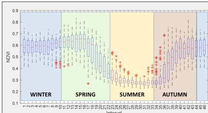
In Fig. 4, box plots of all RVs with a start and end reference of the astronomical seasons are shown. The typical evolution of the NDVI throughout a year can be seen together with the interquartile range.
The observed evolution of NDVI through the different seasons is typical of the pasture in this area. The summer presents the lowest mean values which begin to increase in autumn, achieving a maximum mean value of 0.60 or 0.65 during the beginning of spring. In the middle of the spring NDVIs decrease again, approaching the lowest mean value of 0.28 approximately in summer.
Taking into account these values, dense vegetation, in this study pasture, is found from the middle of October (inter-val 37) until the end of May (inter(inter-val 19). It is in this period where the precipitation concentrates (see Table 1). During the summer, the NDVI mean values are lower than 0.3, cor-responding with low precipitation and high temperatures.
Following the work of Escribano-Rodríguez et al. (2014), there is a relationship of pasture damage and a NDVI value around 0.40. Even if the authors point out that this value is highly variable depending on the location, we can see that the summer season in this case study is under this value (see Fig. 4). This can explain that insurances for damaged pas-ture usually do not apply during these dates due to the arid environment (BOE, 2013).
The statistical metric used in this study to assess the fit of the observed NDVI values with respect to the PDF can-didates (normal, gamma, beta and GEV) was the Chi-square test (χ2test). The following steps were carried out:
1. MLM was applied to model these 46 RVs. Parameters were calculated for the four PDF candidates (see Ta-ble 2).
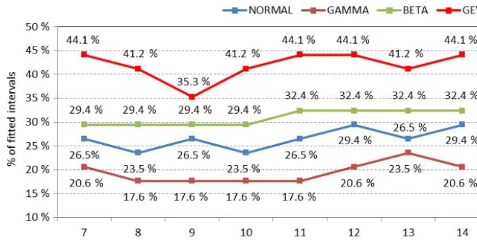
2. To check the goodness of the fit of the PDF candi-dates, a Chi-square test (χ2test) was applied from 7 to 14 classes meeting the requirement that each class have at least five observations. The level of significance (α) was fixed to 5 % for all the candidates.
3.2.1 Maximum likelihood method
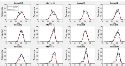
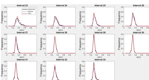
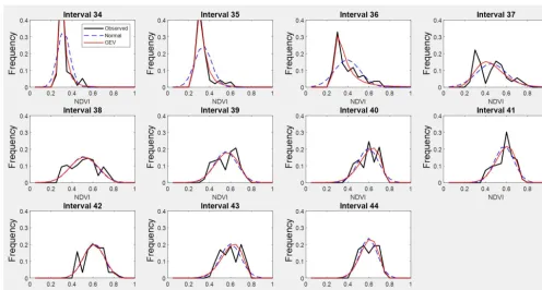
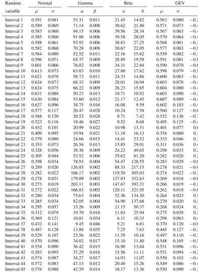
Table A1 shows the estimated parameters for each PDF and each interval calculated by the MLM. These parameters were used to compare the estimated PDF with the NDVI observed values on different times through the seasons. The following intervals are shown as examples of better GEV fit: interval 4 and 8 (for winter, see Fig. 5), interval 17 and 21 (for spring, see Fig. 6), and interval 36 and 40 (for autumn, see Fig. 7). In these plots, observed frequency is compared versus normal and GEV density distributions calculated by MLM.
During winter (see Fig. 5) the observed NDVI distribution presents negative skewness. Then, there is a higher frequency of high NDVI values corresponding with significant precip-itation. During spring (see Fig. 6) an evolution in the skew-ness is observed passing from negative to positive, and so the lower NDVI values become more probable. Finally, during autumn (see Fig. 7) precipitation begins, the skewness passes from positive to negative values, and so higher NDVI values are possible again. We can observe that the normal tion has no flexibility to follow this dynamic in the distribu-tions for each time. This comparison is done in a sequential order for the whole of intervals in Figs. A1–A4.
3.2.2 χ2test
Twelve intervals (from 23 to 34) corresponding to the months of July, August and September have been excluded in this analysis since these intervals fall into the dry season in the study area, which is normally not covered by any SIBI. Therefore, calculations were carried out over 34 intervals.
Figure 4.Box plots of 46 random variables (RVs) are shown as well as the start and end reference of every season. The study period ranges from 2002 to 2017.
Figure 5.Comparison between observed NDVI frequency, GEV and normal probability density functions (PDFs) on two different dates. Intervals 4 and 8 are examples for winter.
Figure 6.Comparison between observed NDVI frequency, GEV and normal probability density functions on two different dates. Intervals 17 and 21 are examples for spring.
4 Discussion
4.1 Statistical context
analy-Figure 7.Comparison between observed NDVI frequency, GEV and normal probability density functions on two different times. Intervals 36 and 41 are examples for autumn.
Figure 8.Percentage of fitted intervals (yaxis) for each PDF candidate (normal, gamma, beta and GEV distributions) as a function of the number of classes (xaxis).
sis) than the normal, gamma or beta distributions. An impor-tant difference between the normal distribution and the PDFs used in this work is their skewness and kurtosis. Many of the observed NDVI distributions present a clear asymmetry and long tails in one or both sides that cause normal distributions not to be the optimal fit.
There is a relationship between seasons and the number of intervals that fit correctly. We found that GEV distributions explain intervals of spring and autumn better since their ob-served distributions are very asymmetric. On the other hand, we did not find an important difference in winter, since the observed distributions are mainly symmetric.
The more skewness and kurtosis depart from those of the normal distribution, the larger the errors affecting the insur-ance designed based on normal distributions (Turvey and Mclaurin, 2012). It is an expected result as pasture cultiva-tion is quite different from the development of arable crops, where normal distributions in the NDVI values are more common. This high heterogeneity in time and space of NDVI estimated on pasture has been pointed out in several works
(Martin-Sotoca et al., 2018). At the same time, the more dif-ferent the observed NDVI frequency is from a normal dis-tribution, the less representative the average is, and so the median becomes a more representative value.
4.2 Insurance context
The use of NDVI thresholds in a damaged pasture context was presented in the introduction section, being an exam-ple of using the insurance for damaged pasture in Spain (BOE, 2013). We have chosen this last insurance to com-pare the results between applying normal and GEV distribu-tion methodologies. In this particular case the NDVI thresh-old (NDVIth) was calculated using the expression NDVIth= µ−k·σ(whereµandσ are the average and standard devia-tion of NDVI distribudevia-tions respectively, assuming the normal hypothesis).
Ta-Table 4.First column: time intervals of approximately 8 d through-out the year. Second column: NDVI thresholds (NDVIth) based on
a normal distribution applyingµ−0.7×σ. Third column: percent-ages of area below the NDVIthwhen normal distributions are
ap-plied. Fourth column: percentages of area below the NDVIthwhen
GEV distributions are applied. Fifth column: relative area error of GEV compared to the normal distribution.
Random Normal GEV variable NDVIth Prob. Prob. Error (%)
Interval 1 0.535 24.20 % 24.37 % 0.70 % Interval 2 0.541 24.20 % 23.18 % −4.21 % Interval 3 0.541 24.20 % 23.27 % −3.84 % Interval 4 0.543 24.20 % 23.27 % −3.84 % Interval 5 0.545 24.20 % 24.17 % −0.12 % Interval 6 0.534 24.20 % 21.48 % −11.24 % Interval 7 0.528 24.20 % 24.01 % −0.79 % Interval 8 0.546 24.20 % 20.70 % −14.46 % Interval 9 0.555 24.20 % 21.30 % −11.98 % Interval 10 0.561 24.20 % 22.28 % −7.93 % Interval 11 0.567 24.20 % 23.49 % −2.93 % Interval 12 0.572 24.20 % 23.75 % −1.86 % Interval 13 0.571 24.20 % 23.20 % −4.13 % Interval 14 0.570 24.20 % 24.29 % 0.37 % Interval 15 0.571 24.20 % 23.47 % −3.02 % Interval 16 0.560 24.20 % 23.26 % −3.88 % Interval 17 0.495 24.20 % 21.29 % −12.02 % Interval 18 0.484 24.20 % 21.58 % −10.83 % Interval 19 0.442 24.20 % 23.06 % −4.71 % Interval 20 0.381 24.20 % 27.20 % 12.40 % Interval 21 0.342 24.20 % 29.46 % 21.74 % Interval 22 0.323 24.20 % 28.84 % 19.17 % Interval 35 0.257 24.20 % 18.98 % −21.57 % Interval 36 0.285 24.20 % 28.57 % 18.06 % Interval 37 0.333 24.20 % 25.90 % 7.02 % Interval 38 0.398 24.20 % 24.27 % 0.29 % Interval 39 0.454 24.20 % 23.79 % −1.69 % Interval 40 0.503 24.20 % 22.81 % −5.74 % Interval 41 0.491 24.20 % 23.23 % −4.01 % Interval 42 0.517 24.20 % 24.66 % 1.90 % Interval 43 0.507 24.20 % 23.13 % −4.42 % Interval 44 0.514 24.20 % 23.49 % −2.93 % Interval 45 0.515 24.20 % 23.70 % −2.07 % Interval 46 0.509 24.20 % 23.33 % −3.60 %
ble 4). The probability of being below NDVIthhas also been calculated using GEV distributions obtained in this study. The probability obtained by GEV distributions is mostly lower than the normal distributions in spring, autumn and winter (see Table 4), which the working period of the insur-ance.
Observing where in time the highest relative errors in probabilities are (fifth column in Table 4), intervals corre-sponding to the end of winter, the second half of spring and the beginning of autumn present errors higher than 10 %. This could explain why it is in spring and autumn when more
Table 5.First column: time intervals of approximately 8 d through-out the year. Second column: NDVI thresholds (NDVIth) based on
a normal distribution (normal) applyingµ−0.7×σ. Third column: NDVIthbased on a GEV distribution (GEV) using 24.2 % as the
area below the NDVIth. Fourth column: relative NDVIth error of
GEV compared to the normal distribution.
Random NDVIth Error (%)
variable Normal GEV
Interval 1 0.535 0.534 −0.19 % Interval 2 0.541 0.543 0.37 % Interval 3 0.541 0.543 0.37 % Interval 4 0.543 0.545 0.37 % Interval 5 0.545 0.545 0.00 % Interval 6 0.534 0.543 1.69 % Interval 7 0.528 0.528 0.00 % Interval 8 0.546 0.558 2.20 % Interval 9 0.555 0.563 1.44 % Interval 10 0.561 0.567 1.07 % Interval 11 0.567 0.569 0.35 % Interval 12 0.572 0.574 0.35 % Interval 13 0.571 0.574 0.53 % Interval 14 0.570 0.569 −0.18 % Interval 15 0.571 0.573 0.35 % Interval 16 0.560 0.563 0.54 % Interval 17 0.495 0.510 3.03 % Interval 18 0.484 0.498 2.89 % Interval 19 0.442 0.447 1.13 % Interval 20 0.381 0.374 −1.84 % Interval 21 0.342 0.334 −2.34 % Interval 22 0.323 0.318 −1.55 % Interval 35 0.257 0.262 1.95 % Interval 36 0.285 0.278 −2.46 % Interval 37 0.333 0.327 −1.80 % Interval 38 0.398 0.398 0.00 % Interval 39 0.454 0.455 0.22 % Interval 40 0.503 0.508 0.99 % Interval 41 0.491 0.494 0.61 % Interval 42 0.517 0.516 −0.19 % Interval 43 0.507 0.510 0.59 % Interval 44 0.514 0.516 0.39 % Interval 45 0.515 0.516 0.19 % Interval 46 0.509 0.511 0.39 %
disagreements exist between farmers and insurance company in claims.
An alternative calculation can be the use of normal proba-bility (24.2 %) to calculate new NDVIthbased on GEV (see Table 5). It can be seen that the new NDVIthvalues obtained by GEV distributions are mostly higher than thresholds using normal distributions in spring, autumn and winter. Consider-ing these results we find that damage thresholds calculated by GEV distributions are mostly above the ones calculated by normal distributions.
NDVIth relative errors higher than 1 % in absolute values (fourth column in Table 5).
5 Conclusions
According to the results obtained in the study area using MLM and theχ2test, it can be concluded that normal dis-tributions are not a good fit to the NDVI observations, and GEV distributions provide a better approximation.
The difference between the normal and GEV assumption is more evident in the transition from winter to summer (spring), where NDVI values decrease, and then from sum-mer to winter (autumn) presenting the opposite behavior of increasing NDVI values. In both periods, asymmetrical dis-tributions were found – negative skewness for the spring tran-sition and positive skewness for the autumn trantran-sition. Dur-ing both periods the variability in precipitation and tempera-tures were higher in this location.
We have found differences if GEV assumption is selected instead of the normal one when defining damaged pasture thresholds (NDVIth). The use of these different assumptions should be taken into account in future insurance implemen-tations due to the important consequences of supposing a damage event or not. We propose the use of quantiles in observed NDVI distributions instead of average and stan-dard deviation, typically of normal distributions, to calculate new NDVIth.
Appendix A
Figure A2.Observed NDVI, GEV and normal probability density functions from interval 11 to interval 22 (from 22 March to 25 June) representing spring.
Table A1.Maximum likelihood parameters calculated for four PDFs.
Random Normal Gamma Beta GEV
variable µ σ α β a b µ σ ξ
Author contributions. JMS developed the research idea and wrote the original draft of the manuscript, guided and supervised by ASR, RM, ND, IF and AMT. ASR contributed in the image filter design. AMT contributed with the imagery and statistical analysis. RM ob-tained the agro-meteorological and vegetation data for the classi-fication of the area. ND and IF contributed in the introduction of index-based insurances and vegetation indexes, as well as in the setting of the vegetation index thresholds. AMT, ASR and RM re-viewed and edited the manuscript for obtaining the final version.
Competing interests. The authors declare that they have no conflict of interest.
Special issue statement. This article is part of the special issue “Re-mote sensing, modelling-based hazard and risk assessment, and management of agro-forested ecosystems”. It is a result of the EGU General Assembly, Vienna, Austria, 8–13 April 2018.
Acknowledgements. This research has been partially supported by funding from MINECO under contract no. MTM2015-63914-P and CICYT PCIN-2014-080. The last author is grateful to the Comunidad de Madrid (Spain) and Structural Funds 2014–2020 (ERDF and ESF) for the financial support (project AGRISOST-CM S2018/BAA-4330) and EU project 821964 – BEACON.
Review statement. This paper was edited by Anne Gobin and re-viewed by three anonymous referees.
References
AEMET: OpenData. Sistema para la difusión y reutilización de la información de AEMET, available at: https://opendata.aemet.es/ centrodedescargas/inicio (last access: 2 August 2019), 2017. Al-Bakri, J. T. and Taylor, J. C.: Application of NOAA AVHRR for
monitoring vegetation conditions and biomass in Jordan, J. Arid Environ, 54, 579–593, 2003.
Anyamba, A., and Tucker, C. J.: Historical perspective of AVHRR NDVI and vegetation drought monitoring, in: Re-mote Sensing of Drought: Innovative Monit Approaches, CRC Press/Taylor & Francis, Florida, USA, 23–50, 2012. Bailey, S.: The Impact of Cash Transfers on Food Consumption
in Humanitarian Settings: A review of evidence, Study for the Canadian Foodgrains Bank, Canadian Foodgrains Bank, Win-nipeg, Canada, May 2013.
Bayarjargal, Y., Karnieli, A., Bayasgalan, M., Khudulmur, S., Gan-dush, C., and Tucker, C. J.: A comparative study of NOAA-AVHRR derived drought indices using change vector analysis, Remote Sens. Environ., 105, 9–22, 2006.
BOE – Boletin Oficial del Estado: 6638 – Orden AAA/1129/2013, No. 145, III, p-46077, Gobierno de España, Madrid, Spain, 2013. Cochran, W. G.: The Chi-square Test of Goodness of Fit, Ann.
Math. Stat., 23, 315–345, 1952.
Crimmins, M. A. and Crimmins, T. M.: Monitoring plant phenology using digital repeat photography, Environ. Manage., 41, 949– 958, 2008.
Dalezios, N. R.: The Role of Remotely Sensed Vegetation Indices in Contemporary Agrometeorology, Invited paper in Honorary Special Volume in memory of late Prof. A. Flokas, Hellenic Me-teorological Association, Athens, Greece, 33–44, 2013. Dalezios, N. R., Blanta, A., Spyropoulos, N. V., and Tarquis, A.
M.: Risk identification of agricultural drought for sustainable Agroecosystems, Nat. Hazards Earth Syst. Sci., 14, 2435–2448, https://doi.org/10.5194/nhess-14-2435-2014, 2014.
De Leeuw, J., Vrieling, A., Shee, A., Atzberger, C., Hadgu, K. M., Biradar, C. M., Humphrey Keah, H., and Turvey, C.: The Po-tential and Uptake of Remote Sensing in Insurance: A Review, Remote Sens., 6, 10888–10912, 2014.
Escribano Rodríguez, A., Díaz-Ambrona, J., Carlos, G. H., and Tar-quis Alfonso, A. M.: Selection of vegetation indices to estimate pasture production in Dehesas, PASTOS, 44, 6–18, 2014. Fensholt, R. and Proud, S. R.: Evaluation of earth observation based
global long term vegetation trends - comparing GIMMS and MODIS global NDVI time series, Remote Sens. Environ., 119, 131–147, 2012.
Flynn, E. S.: Using NDVI as a pasture management tool, MS Thesis, University of Kentucky, Kentucky, 2006.
Forkel, M., Carvalhais, N., Verbesselt, J., Mahecha, M. D., Neigh, C. S., and Reichstein, M.: Trend change detection in NDVI time series: effects of inter-annual variability and methodology, Re-mote Sens., 5, 2113–2144, 2013.
Fuller, D. O.: Trends in NDVI time series and their relation to range-land and crop production in Senegal, 1987–1993, Int. J. Remote Sens., 19, 2013–2018, 1998.
Gommes, R. and Kayitakire, F.: The challenges of index-based in-surance for food security in developing countries, in: Proceed-ings, Technical Workshop, JRC, 2–3 May 2012, JRC-EC, Ispra, p. 276, 2013.
Gouveia, C., Trigo, R. M., and DaCamara, C. C.: Drought and vege-tation stress monitoring in Portugal using satellite data, Nat. Haz-ards Earth Syst. Sci., 9, 185–195, https://doi.org/10.5194/nhess-9-185-2009, 2009.
Goward, S. N., Tucker, C. J., and Dye, D.G.: North-American veg-etation patterns observed with the NOAA-7 advanced very high-resolution radiometer, Vegetation, 64, 3–14, 1985.
Graham, E. A., Yuen, E. M., Robertson, G. F., Kaiser, W. J., Hamil-ton, M. P., and Rundel, P. W.: Budburst and leaf area expansion measured with a novel mobile camera system and simple color thresholding, Environ. Exp. Bot., 65, 238–244, 2009.
Hobbs, T. J.: The use of NOAA-AVHRR NDVI data to assess herbage production in the arid rangelands of central Australia, Int. J. Remote Sens., 16, 1289–1302, 1995.
Holben, B. N.: Characteristics of maximum-value composite im-ages from temporal AVHRR data, Int. J. Remote Sens., 7, 1417– 1434, 1986.
Kottek, M., Grieser, J., Beck, C., Rudolf, B., and Rubel, F.: World Map of the Köppen-Geiger climate classification updated, Mete-orol. Z., 15, 259–263, 2006.
Larson, H. J.: Introduction to Probability Theory and Statistical In-ference, 3rd Edn., John Wiley and Sons, New York, 1982. Leblois, A.: Weather index-based insurance in a cash crop regulated
sector: ex ante evaluation for cotton producers in Cameroon, in: Paper presented at the JRC/IRI workshop on The Challenges of Index-Based Insurance for Food Security in Developing Coun-tries, 2–3 May 2012, Ispra, 2012.
Li, R., Tsunekawa, A., and Tsubo, M.: Index-based assessment of agricultural drought in a semi-arid region of Inner Mongolia, China, J. Arid Land, 6, 3–15, 2014.
Lovejoy, S., Tarquis, A. M., Gaonac’h, H., and Schertzer, D.: Sin-gle and Multiscale remote sensing techniques, multifractals and MODIS derived vegetation and soil moisture, Vadose Zone J., 7, 533–546, 2008.
LP DAAC – Land Processes Distributed Active Archive Center: Surface Reflectance 8-Day L3 Global 500 m, NASA and USGS, available at: https://lpdaac.usgs.gov/products/mod09a1v006/ (last access: 2 August 2019), 2014.
Maples, J. G., Brorsen, B. W., and Biermaches, J. T.: The rainfall Index Annual Forage pilot program as a risk management tool for cool-season forage, J. Agr. Appl Econ, 48, 29–51, 2016. Martin-Sotoca, J. J., Saa-Requejo, A., Orondo J. B., and Tarquis,
A. M.: Singularity maps applied to a vegetation index, Bio. Eng., 168, 42–53, 2018.
Motohka, T., Nasahara, K. N., Murakami, K., and Nagai, S.: Evalu-ation of sub-pixel cloud noises on MODIS daily spectral indices based on in situ measurements, Remote Sens., 3, 1644–1662, 2011.
Nanzad, L., Zhang, J., Tuvdendorj, B., Nabil, M., Zhang, S., and Bai, Y.: NDVI anomaly for drought monitoring and its correla-tion with climate factors over Mongolia from 2000 to 2016, J. Arid Environ., 164, 69–77, 2019.
Niemeyer, S.: New drought indices, in: First Int. Conf. on Drought Management: Scientific and Technological Innova-tions, Zaragoza, Spain, Joint Research Centre of the European Commission, available at: http://projects.iamz.ciheam.org/ medroplan/zaragoza2008/Sequia2008/Session3/S.Niemeyer.pdf (last access: 2 August 2019), 2008.
Ortega-Farias, S., Ortega-Salazar, S., Poblete, T., Kilic, A., Allen, R., Poblete-Echeverría, C., Ahumada-Orellana, L., Zuñiga, M., and Sepúlveda, D.: Estimation of Energy Balance Components over a Drip-Irrigated Olive Orchard Using Thermal and Mul-tispectral Cameras Placed on a Helicopter-Based Unmanned Aerial Vehicle (UAV), Remote Sens., 8, 638, 2016.
Park, S.: Cloud and cloud shadow effects on the MODIS vegetation index composites of the Korean Peninsula, Int. J. Remote Sens., 34, 1234–1247, 2013.
Peters, A. J., Walter-Shea, E. A., Ji, L., Vina, A., Hayes, M., and Svoboda, M. D.: Drought monitoring with NDVI-Based Stan-dardized Vegetation Index, Photogram. Eng. Remote Sens., 68, 71–75, 2002.
Rao, K. N.: Index based Crop Insurance, Agric. Agric. Sci. Proc., 1, 193–203, 2010.
Roumiguié, A., Jacquin, A., Sigel, G., Poilvé, H., Lepoivre, B., and Hagolle, O.: Development of an index-based insurance product: validation of a forage production index derived from medium spatial resolution fCover time series, GIScience Remote Sens., 52, 94–113, 2015.
Roumiguié, A., Sigel, G., Poilvé, H., Bouchard, B., Vrieling, A., and Jacquin, A.: Insuring forage through satellites: testing alter-native indices against grassland production estimates for France, Int. J. Remote Sens., 38, 1912–1939, 2017.
Tackenberg, O.: A New Method for Non-destructive Measurement of Biomass, Growth Rates, Vertical Biomass Distribution and Dry Matter Content Based on Digital Image Analysis, Ann. Bot., 99, 777–783, 2007.
Turvey, C. G. and Mclaurin, M. K.: Applicability of the Normal-ized Difference Vegetation Index (NDVI) in Index-Based Crop Insurance Design, Am. Meorol. Soc., 4, 271–284, 2012. UNEP Word Atlas of Desertification: Second Ed. United Nations
Enviroment Programe, Nairobi, 1997.
USDA – US Department of Agriculture, Federal Crop Insurance Corporation, Risk Management Agency: Rainfall Index Plan Annual Forage Crop Provisions, 16-RI-AF, available at: http: //www.rma.usda.gov/policies/ri-vi/2015/16riaf.pdf2013, last ac-cess: 1 March 2018.