PID control as a process of active inference with
linear generative models
Manuel Baltieri†,‡ and Christopher L. Buckley‡
EASy group - Sussex Neuroscience, Department of Informatics, University of Sussex, Brighton, UK; [email protected], [email protected]
* Correspondence: [email protected]
† This paper is an extended version of our paper published in From Animals to Animats 15: 15th International Conference on Simulation of Adaptive Behavior, SAB 2018.
Version February 27, 2019 submitted to Preprints
Abstract: In the past few decades, probabilistic interpretations of brain functions have become 1
widespread in cognitive science and neuroscience. In particular, the free energy principle and 2
active inference are increasingly popular theories of cognitive functions that claim to offer a 3
unified understanding of life and cognition within a general mathematical framework derived 4
from information and control theory, and statistical mechanics. However, we argue that if the active 5
inference proposal is to be taken as a general process theory for biological systems, it is necessary 6
to understand how it relates to existing control theoretical approaches routinely used to study and 7
explain biological systems. For example, recently, PID control has been shown to be implemented in 8
simple molecular systems and is becoming a popular mechanistic explanation of behaviours such 9
as chemotaxis in bacteria and amoebae, and robust adaptation in biochemical networks. In this 10
work, we will show how PID controllers can fit a more general theory of life and cognition under 11
the principle of (variational) free energy minimisation when using approximate linear generative 12
models of the world. This more general interpretation provides also a new perspective on traditional 13
problems of PID controllers such as parameter tuning as well as the need to balance performances 14
and robustness conditions of a controller. Specifically, we then show how these problems can be 15
understood in terms of the optimisation of the precisions (inverse variances) modulating different 16
prediction errors in the free energy functional. 17
Keywords: approximate Bayesian inference, active inference, PID control, generalised state-space 18
models, sensorimotor loops, information theory, control theory 19
1. Introduction 20
Probabilistic approaches to the study of living systems and cognition are becoming increasingly 21
popular in the natural sciences. In particular for the brain sciences, the Bayesian brain hypothesis, 22
predictive coding, the free energy principle and active inference have been proposed to explain 23
brain processes including perception, action and higher order cognitive functions [1–8]. According
24
to these theories, brains, and biological systems more generally, should be thought of as Bayesian 25
inference machines, since they appear to estimate the latent states of their sensory input in a process 26
consistent with a Bayesian inference scheme. Given the complexity of exact Bayesian inference, 27
however, approximated schemes are believed to provide a more concrete hypothesis on the underlying 28
mechanisms. One candidate scheme is the free energy principle (FEP), which was introduced in [4] and
29
later elaborated in a series of papers, e.g. [9–11], and has its roots in information theory, control theory, 30
thermodynamics and statistical mechanics. While initially the theory emerged in the computational 31
[12] and behavioural/cognitive neurosciences [13,14], over time, further connections with the fields of
32
biological self-organisation, information theory, optimal control, cybernetics and economics among 33
others, have also been suggested [10,15–17]. According to the FEP, living systems exist in a limited
34
set of physical states and thus must minimise the entropy of those physical states (see fluctuation 35
theorems for non-equilibrium thermodynamics, e.g. [18]). To achieve this, organisms can minimise the 36
informational entropy of their sensory states, which, under ergodic assumptions, is equivalent to the 37
time average ofsurprisal(or self-information) [9]. Surprisal quantifies how improbable an outcome
38
is for a system, i.e. a fish out of water is in a surprising state. Biological creatures can thus be seen 39
as minimising the surprisal of their sensations to maintain their existence, e.g. a fish’ observations 40
should be limited to states in water. Since this surprisal itself is not directly accessible by an agent, 41
variational free energy is proposed as an upper bound on this quantity which can be minimised in its 42
stead [4,19]. It has also been suggested that cognitive functions such as perception, action, learning
43
and attention can be accounted for in terms approximate Bayesian inference schemes such as the FEP. 44
In particular, according to this hypothesis, perception can be described using predictive coding models 45
of the cortex. These models describe perception as a combination of feedforward prediction errors 46
and feedback predictions combined under a generative model to infer the hidden causes and states 47
of sensory data [2]. More recent work has connected these ideas to control theory and cybernetics
48
[15,17,20], extending existing accounts of (optimal) motor control and behaviour [10,13,21,22]. On this 49
view, behaviour is cast as a process of acting on the world to make sensory data better fit existing 50
predictions, with (optimal) motor control cast as a Bayesian inference problem. The most recent 51
attempt to unify predictive coding and optimal control theory, usually falls under the name ofactive
52
inference[10,13]. 53
While in standard accounts of perceptual inference prediction errors can be suppressed only by 54
updating predictions of the incoming sensations, in active inference errors can also be minimised by 55
directly acting on the environment to change sensory input to better accord with existing predictions 56
[9,13]. If a generative model encodes information about favourable states for an agent, then this
57
process constitutes a way by which the agent can change its environment to better meet its needs. Thus, 58
under the FEP, these two processes of error suppression allow a system to both infer the properties of, 59
and control, the surrounding environment. Most models implementing the FEP and active inference 60
assume that agents have a deep understanding of their environment and its dynamics in the form of 61
an accurate and detailed generative model. For instance, in [13,23] the generative model of the agent
62
explicitly mirrors thegenerative processof the environment, i.e. the dynamics of the world the agent
63
interacts with. In recent work, it has been argued that this need not be the case [24–27], especially if we 64
consider simple living systems with limited resources. We intuitively don’t expect an ant to model 65
the entire environment where it forages, performing complex simulations of the world in its brain (cf. 66
the concept of Umwelt [28]). When states and parameters in the world change too rapidly, accurate
67
online inference and learning are implausible [29]. This idea is however common in the literature,
68
e.g. [6,13,14,23], where cognition and perception are presented as processes of inference to the best
69
explanation, and agents are primarily thought to build sophisticated models of their worlds with only 70
a secondary role for action and behaviour. A possible alternative introduces action-oriented models 71
entailing a more parsimonious approach where only task-relevant information is encoded [24,25]. On
72
this normative view, agents only model a minimal set of environmental properties, perhaps in the 73
form of sensorimotor contingencies [26], that are necessary to achieve their goals.
74
The relationship between information/probability theory and control theory has long been 75
recognised, with the first intuitions emerging from work by Shannon [30] and Kalman [31]. A unifying
76
view of these two theoretical frameworks is nowadays proposed for instance in stochastic optimal 77
control [32,33] and extended in active inference [15], with connections to ideas of sensorimotor loops in 78
biological systems [11,13]. These connections emphasise homeostasis, regulation and concepts such as
79
set-point control and negative feedback for the study of different aspects of living systems, with roots 80
in the cybernetics movement [34,35]. It remains, however, unclear how the active inference formulation
81
directly relates to more traditional concepts of control theory. PID control, a popular control strategy 82
working with little prior knowledge of the process to regulate, is commonly applied in engineering 83
[36–38] and more recently used in biology and neuroscience modelling [39–43]. In this work, we
84
more general Bayesian (active) inference framework. We will show that approximate models of the 86
world are often enough for regulation, and in particular that simple linear generative models that only 87
approximate the true dynamics of the environment implement PID control as a process of inference. 88
Using this formulation we also propose a new method for the optimisation of the gains of PID 89
controllers based on the same principle of variational free energy minimisation, and implemented as a 90
second order optimisation process. Finally, we will show that our implementation of PID controllers as 91
approximate Bayesian inference lends itself to a general framework for the formalisation of different 92
(conflicting) criteria in the design of a controller, the so-called performance-robustness trade-off 93
[38,44], as a cohesive set of constraints implemented in a free energy functional. In active inference,
94
these criteria will be mapped to precisions, or inverse variances, of observations and dynamics of a 95
state-space model with a straightforward interpretation in terms of uncertainty on different variables 96
of a system. 97
In section2we will introduce PID control and give a brief overview of the recent literature
98
highlighting the most common design principles used nowadays for PID controllers. The free energy 99
principle will be presented in section3, followed by a complete derivation of PID control as a form
100
of active inference. In this section we will also propose that the parameters of a PID controller, its 101
gains, can be optimised following the active inference formulation, which also captures modern design 102
constraints and desiderata of PID controllers. 103
2. PID control 104
Proportional-Integral-Derivative (PID) control is one of the most popular types of controllers used in industrial applications, with more than 90% of total controllers implementing PID or PI (no derivative) regulation [38,45]. It is one of the simplest set-point regulators, whereby a desired state (i.e. set-point, reference, target) represents the final goal of the regulation process, e.g. to maintain a room
temperature of 23◦C. PID controllers are based on closed-loop strategies with a negative feedback
mechanism that tracks the real state of the environment. In the most traditional implementation of negative feedback methods, the difference between the measured state of the variable to regulate (e.g.
the real temperature in a room) and the target value (e.g. 23◦C) produces a prediction error whose
minimisation drives the controller’s output, e.g. if the temperature is too high, it is decreased and if too low, it is raised. In mathematical terms:
e(t) =yr−y(t) (1)
wheree(t)is the error,yris thereferenceor set-point (e.g. desired temperature) andy(t)is the observed 105
variable (e.g. the actual room temperature). 106
This mechanism is, however, unstable in very common conditions, in particular when a steady-state offset is added (e.g. a sudden and unpredictable change in external conditions affecting the room temperature which are not under our control), or when fluctuations need to be suppressed (e.g. too many oscillations while regulating the temperature may be undesirable). PID controllers elegantly deal with both of these problems by augmenting the standard negative feedback architecture, here calledproportionalorP term, with anintegralorIand aderivativeorD term, see Fig.1. The integral term accumulates the prediction error over time in order to cancel out errors due to unaccounted steady-state input, while minimising the derivative of the prediction error leads to a decrease in the
amplitude of fluctuations of the controlled signal. The general form of the control signalu(t)generated
by a PID controller is usually described by:
u(t) =kpe(t) +ki
Z t
0 e
(τ)dτ+kd de(t)
dt (2)
wheree(t) is, again, the prediction error andkp,ki,kd are the so called proportional, integral and
107
terms of the controller. The popularity of PID controllers is largely due to their simple formulation and
Figure 1. A PID controller [46].The prediction errore(t)is given by the difference between a reference signalr(t),yrin our formulation, and the outputy(t)of a process. The different terms, one proportional to the error (P term), one integrating the error over time (I term) and one differentiating it (D term), drive the control signalu(t).
109
implementation. One of the major challenges on the other hand, lies with the tuning of parameters 110
kp,ki,kd, that have to be adapted to deal with different (often conflicting) constraints on the regulation 111
process [36,44]. 112
2.1. The performance-robustness trade-off 113
The presence of conflicting criteria for the design of PID controller is a well known issue in the 114
control theory literature, often referred to as the performance-robustness trade-off [38,44,47–49]. A
115
controller needs to optimise pre-specified performance criteria while, at the same time, preserving some 116
level of robustness in face of uncertainty and unexpected conditions during the regulation process. 117
In recent attempts to formalise and standardise these general principles [38,44], the performance of a
118
controller has been proposed to be evaluated through: 119
• load disturbance response, how a controller reacts to changes in external inputs, e.g. a step input,
120
• set-point response, how a controller responds to different set-points over time,
121
• measurement noise response, how noise on the observations impacts the regulation process,
122
while robustness to be assessed on: 123
• robustness to model uncertainty, how uncertainty on the plant/environment dynamics affects
124
the controller. 125
The goal of a general methodology for the design and tuning of PID controllers is to bring together 126
these (and possibly more) criteria into a formal and tractable framework that can be used for a large 127
class of problems. One possible example is presented in [48] (see also [50,51] for other attempts). This
128
methodology is based on the maximisation of the integral gain (equivalent to the minimisation of 129
the integral of the error from the set-point, see [36]), subject to constraints derived from a frequency
130
domain analysis related to the Nyquist stability criterion applied to the controlled system [48]. In
131
this work, we propose our formulation also as a general framework for the design and tuning of 132
PID controllers leveraging the straightforward interpretation of the performance-robustness trade-off 133
for PID controllers in terms of uncertainty parameters (i.e. precisions or inverse variances) in the 134
variational free energy. 135
3. The active inference framework 136
According to the free energy principle, living system must minimise the surprisal, or self-information, of their observations [4,9,10,19], defined as:
whereψis a set of sensory inputs conditioned on an agentm. Surprisal, in general, can in fact differ
from agent to agent, with states that are favourable for a fish (in water), different from those favourable
for a bird (out of water) (see [52] for a review on the value of information). According to the FEP, agents
that minimise the surprisal of their sensory states over time will also minimise the entropy of their
sensations, thus limiting the number of states they can physically occupy [4,19]. This minimisation is,
however, intractable in any practical scenario since surprisal can be seen as the negative log-model
evidence or negative log-marginal likelihood of observationsψ, with (omittingmfor simplicity from
now on) the marginal likelihood or model evidence expressed as:
p(ψ) =
Z
ϑ
p(ψ,ϑ)dϑ. (4)
This integral is defined over all possible hidden variables,ϑ, of observationsψ. In many cases, the
marginalisation is intractable since the latent space ofϑmay be high dimensional or the distribution
may have a complex (analytical) form. In statistical mechanics, an approximation under variational formulations transforms this into an optimisation problem. The approximation goes by several names,
including variational Bayes and ensemble learning [53,54], and constitutes the mathematical basis of
the free energy principle. Using variational Bayes, surprisal can then be decomposed into [54]:
−lnp(ψ) =F−DKL(q(ϑ)||p(ϑ|ψ)), (5)
where
DKL(q(ϑ)||p(ϑ|ψ)) =
Z
q(ϑ)ln q(ϑ)
p(ϑ|ψ) dϑ, (6)
is the Kullback-Leibler (KL) divergence [55], or relative entropy [54], an asymmetrical non-negative
measure of the difference between two probability distributions. The first one,p(ϑ|ψ), represents the
posterior distribution specifying the probability of hidden states, causes and parameters (ϑ) given
observationsψ, while the second oneq(ϑ), is the variational or recognition density which encodes
currents beliefs over hidden variablesϑ. The latter is introduced with the idea of approximating
the (also) intractable posteriorp(ϑ|ψ)with a simpler distribution,q(ϑ), and then minimising their
difference through the KL divergence: when the difference is zero (following Jensen’s inequality the divergence is always non-negative [54]),q(ϑ)is a perfect description ofp(ϑ|ψ). Analogously, from the
point of view of an agent, its goal is to explain the hidden states, causes and parametersϑof sensations
ψby approximating the posteriorp(ϑ|ψ)with a known distribution,q(ϑ). The first term in equation5
can be written as
F=
Z
q(ϑ)ln q(ϑ)
p(ϑ,ψ) dϑ (7)
and is defined as (variational) free energy [8,12,56,57] for its mathematical analogies with free energy
in thermodynamics, or [54] (negative) evidence lower bound in machine learning. Since the KL
divergence is always non-negative we arrive at
DKL(q(ϑ)||p(ϑ|ψ))≥0⇒F≥ −lnp(ψ) (8)
which demonstrates that variational free energy is an upper bound to surprisal, since by minimisingF
a recognition densityq(ϑ)and a generative densityp(ϑ,ψ)specific to an agent. Starting from the latter,
we define a generative model formulated as a one dimensionalgeneralisedstate-space model [12]:
ψ=g(x,v) +z
ψ0=gx(x,v)x0+gv(x,v)v0+z0
ψ00=gx(x,v)x00+gv(x,v)v00+z00
.. .
˙
x=x0 = f(x,v) +w ˙
x0 =x00= fx(x,v)x0+fv(x,v)v0+w0) ˙
x00=x000 = fx(x,v)x00+fv(x,v)v00+w00) ..
.
(9)
whereψare the observations andϑ={x,v,θ,γ}, withxas the hidden states andvas the exogenous
inputs, whileθandγfollow a partition in terms of parameters and hyperparameters defined in [12]
and are specified later to simplify the notation now. Functionsg(·)and f(·)map hidden states/inputs
to observations and the dynamics of hidden states/inputs respectively. The prime symbols, e.g.
x0,x00,x000are used to define higher orders of motion of a variable. Generalised coordinates of motion
are introduced to represent non-Markovian continuous stochastic processes based on Stratonovich
calculus, with strictly non-zero autocorrelation functions [12,58,59]. Ito’s formulation of stochastic
processes, on the other hand, is based on Wiener noise, where the autocorrelation can be seen as
strictly equal to a delta function [59,60]. In general, the Stratonovich formulation is preferred in
physics, where it is assumed that perfect white noise does not exist in the real world [61], while Ito’s
calculus is extensively used in mathematics/economics for its definition preserving the Martingale
property [62]. It is proposed that models of biological systems should be based on the Stratonovich
derivation [12], to accommodate more realistic properties of the physical world (i.e. non-Markovian
processes). Using the Stratonovich interpretation, random processes can be described as analytic (i.e.
differentiable) and become better approximations of real-world (weakly) coloured noise [60,63,64]. In
this formulation, standard state-space models are extended, describing dynamics and observations for higher “orders of motion” encoding, altogether, a trajectory for each variable. The more traditional state-space description is based on Markovian processes (i.e. white noise) and can be seen as a special
case ofgeneralisedstate-space models defined here and in, for instance, [8,12]. When coloured noise
is introduced, one should either define a high order autoregressive process expressed in terms of
white noise [65] or embrace the Stratonovich formulation defining all the necessary equations in a
state-space form [12]. The higher “orders of motion” introduced here can be thought of as quantities
specifying “velocity” (e.g.(ψ)0), “acceleration” (e.g.(ψ)00), etc. for each variable, which is neglected
in more standard formulations. For practical purposes, in equation (9) we also made a local linearity
approximation on higher orders of motion suppressing nonlinear terms [8,12]. We introduce then a
more compact form:
˜
ψ=g(x˜, ˜v) +z˜ x˜0= f(x˜, ˜v) +w˜ (10)
where the tilde sign (e.g. ψ˜) summarises a variable and its higher orders of motion (e.g. ψ˜ =
{ψ,ψ0,ψ00, . . .}). The stochastic model in equation (9) can then be described in terms of a generative
density:
P(ψ˜, ˜x, ˜v;θ,γ) =P(ψ˜|x˜, ˜v;θ,γ)P(x˜, ˜v;θ,γ) (11)
In this case, we also make the conditional dependence onθ,γexplicit, definingθas slowly changing
parameters coupling hidden states and causes to observations, and hyperparametersγas encoding
properties of random fluctuations/noise ˜wand ˜z.P(ψ|x,v;θ,γ)is a likelihood function describing the
measurement law in equation (10), while the priorP(x˜, ˜v;θ,γ)describes the system’s dynamics. Under
the Laplace approximation [66,67], the form of the recognition densityq(ϑ)is specified in terms of a
Gaussian distribution centred around the estimated mode (i.e. the mean for a Gaussian distributions)
can be solved analytically in terms of the Hessian of the free energy evaluated at the mode [8,67,68].
The variational free energy in equation (7) can then be simplified, without constants, to [8]:
F≈ −lnP(ψ˜, ˜x, ˜v;θ,γ) ˜
ϑ=µ˜ϑ
(12)
where the condition ˜ϑ = µ˜ϑ represents the fact that the generative density P(ψ˜, ˜x, ˜v;θ,γ)will be
approximated by a Gaussian distribution centred around the best estimates ˜µϑ of the unknown ˜ϑ,
following the Laplace method implemented in a variational context [66]. With Gaussian assumptions
on random variables ˜zand ˜win equation equation (10), the likelihood and prior in equation (11) are
also Gaussian, and the variational free energy can be expressed as:
F≈ 1 2
πz˜
˜
ψ−g(µ˜x, ˜µv)
2
+πw˜
˜
µ0x−f(µ˜x, ˜µv)
2
−ln πz˜πw˜
(13)
where ˜x and ˜v are replaced by their sufficient statistics, means/modes ˜µx, ˜µv, and sensory and
dynamics/process precisionsπz,˜ πw, or inverse variances, of random variables ˜˜ zand ˜w. Following
[12,56], the optimisation of the (Laplace-encoded) free energy with respect to expected hidden states
˜
µx, equivalent to estimation or perception, can be implemented via a gradient descent:
˙˜
µx=Dµ˜x−
∂F
∂µ˜x (14)
while, considering how, from the perspective of agent, only observationsψare affected by actionsa
(i.e.ψ(a)), control or action can be cast as:
˙
a=−∂F
∂a =−
∂F
∂ψ˜ ∂ψ˜
∂a (15)
representing a set of coupled differential equations describing a closed sensorimotor loop in terms 137
of a physically plausible minimisation scheme [12]. The first equation includes a term Dµ˜x that
138
represents the “mode of the motion” (also the mean for Gaussian variables) in the minimisation 139
of states in generalised coordinates of motion [8,12,69], with Das a differential operator “shifting”
140
the order of motion of ˜µx such thatDµ˜x = µ˜0x. More intuitively, since we are now minimising the
141
components of a generalised state representing a trajectory rather than a static state, variables are in a 142
moving frame of reference in the phase-space, and the minimisation is achieved when the temporal 143
dynamics of the gradient descent match the ensemble dynamics of the estimates of hidden states, so 144
for ˙˜µx=µ˜0xrather than for ˙˜µx=0 (which assumes that the mode of the motion is zero, as in standard 145
state-space formulations with Markov assumptions). In the second equation, active inference makes 146
the assumption that agents have innate knowledge of the mapping between actionsaand observations
147 ˜
ψ(i.e.∂ψ˜/∂a) as reflex arcs, acquired on an evolutionary time scale, see [13,15] for discussion.
148
4. Results 149
4.1. PID control as active inference 150
To implement PID control as a process of active inference, we will first describe an agent’s generative model as a generalised linear state-space model of second order (i.e. only two higher orders of motion, anything beyond that is zero-mean Gaussian noise):
ψ=x+z
ψ0 =x0+z0
ψ00=x00+z00
˙
x=x0=−α(x+v) +w
˙
x0=x00=−α(x0+v0) +w0
˙
where α ∈ θ is a parameter. As previously suggested, with a Gaussian assumption on ˜z, ˜w, the
likelihood is reduced to:
P(ψ˜|x˜, ˜v;θ,γ) =P(ψ˜|x˜;θ,γ) =N(µ˜x,σz2˜) (16)
where we assume no direct dependence of observations ˜ψon external inputs ˜v, while the prior is
described by:
P(x˜, ˜v;θ,γ) =P(x˜|v˜;θ,γ)P(v˜;θ,γ) (17)
with
P(x˜|v˜;θ,γ) =N(−α(µ˜x+µ˜v),σw2˜)
P(v˜;θ,γ) =N(η˜x,σv2˜) (18)
The Laplace-encoded variational free energy in equation (13) then becomes:
F≈ 1 2
πz
ψ−µx
2
+πz0
ψ0−µ0x
2
+πz00
ψ00−µ00x
2
+πw
µ0x+α(µx−ηx)
2
+
+πw0
µ00x+α(µ0x−ηx0) 2
+πw00
µ000x +α(µ00x−η00x) 2
−ln πzπwπz0πw0πz00πw00
(19)
To simplify our formulation, we assume that precisionsπv˜tend to infinity (i.e. no uncertainty on
the priors for ˜v), so that P(v˜;θ,γ)in equation (18) becomes a delta function and inputs ˜vreduce
to their prior expectations ˜ηx, i.e. µ˜v = η˜x. With this simplification, prior precisions πv˜ and
respective predictions errors(µ˜v−η˜x) are not included in our formulation (see [56,57] for more
general treatments). By applying the gradient descent described in equation (14) and equation (15) to
our free energy functional, we then get the following update equations for perception (estimation):
˙
µx=µ0x−
−πz
ψ−µx
+πwα
µ0x+α(µx−ηx)
˙
µ0x=µ00x−
−πz0
ψ0−µ0x
+πw0α
µ00x+α(µ0x−η0x)
+πw
µ0x+α(µx−ηx)
˙
µ00x =µ000x −
−πz00
ψ00−µ00x
+πw00α
µ000x +α(µ00x−η00x)
+πw0
µ00x+α(µ0x−η0x)
(20)
and for action (control):
˙ a=−
πz
ψ−µx
∂ψ
∂a +πz
0
ψ0−µ0x
∂ψ0
∂a +πz
00
ψ00−µ00x
∂ψ00
∂a
. (21)
The mapping of these equations to a PID control scheme becomes more clear under a few simplifying
assumptions. First, we assume strong priors on the causes of proprioceptive observations ψ1.
Intuitively, these priors are used to define actions that change the observations to better fit the agent’s desires, i.e. the target of the PID controller. This is implemented in the weighting mechanism of
prediction errors by precisions in equation (19); see also [13,26,70] for similar discussions on the
role of precisions for behaviour. In our derivation, weighted prediction errors on system dynamics,
πw˜(µ˜0x+µ˜x−η˜x), will be weighted more than weighted errors on observations,πz˜(ψ˜−µ˜x). To achieve
1 For consistency with previous formulations, e.g. [8,13,15], we will defineψasproprioceptiveobservations. Proprioception is
this, we decrease sensory precisionsπz˜on proprioceptive observations, effectively biasing the gradient
descent procedure towards minimising errors on the prior dynamics [70]. Secondly, we set the decay
parameterαto a large value (theoreticallyα→∞, in practiceα=105in our simulations), obtaining a
set of differential equations including only terms of orderα2for perception:
˙
µx≈ −πwα
α(µx−ηx)
˙
µ0x≈ −πw0α
α(µ0x−η0x)
˙
µ00x ≈ −πw00α
α(µ00x−ηx00)
(22)
This can be interpreted as an agent encoding beliefs in a world that quickly settles to a desired equilibrium state. This assumption effectively decouples orders of generalised motion, with higher
embedding orders not affecting the minimisation of lower ones in equation (20), since terms from
lower orders are modulated byαdirectly. The remaining terms effectively impose constraints on
the generalised motion only close to equilibrium, playing a minor role in the control process away from the target/equilibrium (the more interesting part of regulation). These terms are necessary for
the system to settle to a proper steady state when(µ˜x−η˜x) →0 and maintain consistency across
generalised orders of motion for small fluctuations at steady state, but have virtually no influence at
all in conditions far from equilibrium. Following equation (22), at steady state, expectations on hidden
states ˜µxare mainly driven by priors ˜ηx:
˜
µx=η˜x (23)
but are still not met by appropriate changes in observations ˜ψ which effectively implement the
regulation around the desired target. To minimise free energy in presence of strong priors, this agent
will necessarily have to modify its observations ˜ψto better match expectations ˜µx, which in turn are
shaped by priors (i.e. desires) ˜ηx. Effectively, the agent “imposes” its desires on the world, acting
to minimise the prediction errors arising at the proprioceptive sensory layers. In essence, an active inference agent implements set-point regulation by behaving to make its sensations accord with its strong priors/desires. After these assumptions, action can be written as:
˙ a≈ −
πz
ψ−ηx
∂ψ
∂a +πz
0
ψ0−ηx0
∂ψ0
∂a +πz
00
ψ00−η00x
∂ψ00
∂a
(24)
where we still need to specify partial derivatives∂ψ˜/∂a. As discussed in [13], this step highlights
the fundamental differences between the FEP and the more traditional forward/inverse models
formulation of control problems in biological systems [71,72]. While these derivatives help in the
definition of an inverse model (i.e. finding the correct action for a desired output), unlike more
traditional approaches, active inference does not involve a mapping from hidden states ˜xto actions
a, but is cast in terms of (proprioceptive) sensory data ˜ψdirectly, This is thought to simplify the
problem: from a mapping betweenunknownhidden states and actions, to a mapping betweenknown
proprioceptive observations ˜ψand actionsa. It is claimed that this provides an easier implementation
for an inverse model [15], one that is grounded in an extrinsic frame of reference, i.e. the real world
( ˜ψ), rather than in a intrinsic one in terms of hidden states ( ˜x) to be inferred first. To achieve PID-like
control, we assume that the agent adopts the simplest (i.e. linear) relationship between its actions (controls) and their effects on sensory input across all orders of motion:
∂ψ
∂a =
∂ψ0
∂a =
∂ψ00
∂a =1 . (25)
This reflects a very simple reflex-arc-like mechanism that is triggered every time a proprioceptive
negative actions decrease them. There is, however, an apparent inconsistency here that we need to
dissolve: the proprioceptive inputψand its higher order statesψ0,ψ00arealllinearly dependent with
respect to actionsaas represented in equation (25). While an action may not change position, velocity
and acceleration of a variable in the same way, a generative model doesn’t need to perfectly describe the system to regulate: these derivatives only encode sensorimotor dependencies that allow for, in this case, sub-optimal control. In the same way, PID controllers are, in most cases, effective but only
approximate solutions for control [36,73]. This allows us to understand the encoding of an inverse
model from the perspective of an agent (i.e. the controller) rather than assuming a perfect, objective
mapping from sensations to actions that reflects exactly how actions affect sensory input [13]. This
also points at possible investigations of generative/inverse models in simpler living systems where accurate models are not perhaps needed, and where strategies like PID control are implemented [39–41]. By combining equation (24) and equation (25), action can then be simplified to:
˙
a≈πz ηx−ψ+πz0 ηx0 −ψ0+πz00 η00x−ψ00 (26)
which is consistent with the “velocity form” or algorithm of a PID controller [36]:
˙
u=ki yr−y+kpd
dt yr−y
+kd
d2
dt2 yr−y
. (27)
Velocity forms are used in control problems where, for instance, integration is provided by an external 151
mechanism outside the controller [36,73]. Furthermore, velocity algorithms are the most natural form
152
for the implementation of integral control to avoid windup effects of the integral term, emerging when 153
actuators can’t regulate an indiscriminate accumulation of steady-state error in the integral term due 154
to physical limitations [36,74]. This algorithm is usually described using discrete systems to avoid the
155
definition of the derivative of random variables, often assumed to be white noise in the Ito’s sense 156
(i.e. Markovian processes). In the continuous case, if the variableyis a Markov process, its time
157
derivative is in fact not well defined. For this form to exist in continuous systems,ymust be a smooth
158
(stochastic) process. Effectively, this drops the Markov assumption of white noise and implements 159
the same definition of analytic (i.e. differentiable) noise related to Stratonovich calculus and the 160
generalised coordinates of motion we described earlier. The presence of extra prediction errors beyond 161
the traditional negative feedback (proportional term) can, in this light, be seen as a natural consequence 162
of considering linear non-Markovian processes with simple reflex mechanisms responding to position, 163
velocity and acceleration in the generalised motion phase space (see equation (25)). To ensure that the
164
active inference implementation approximates the velocity form of PID control we still need to clarify 165
the relationship between the generalised coordinates of motion in equation (26) and the differential
166
operatorsd/dt,d2/dt2in equation (27). As pointed out in previous work, when the variational free
167
energy is minimised, the two of them are equal since the motion of the mode becomes the mode of the 168
motion [8,56]. To simplify our formulation and show PID control more directly, we can consider the
169
case forηx0 =η00x =0, defining the more standard set-point control where a desired or set-trajectory
170
collapses to a single set-point in the state-space and equivalent, in the velocity form, to the case where 171
yris a constant anddyr/dt=d2yr/dt2=0. 172
To show an implementation of PID control through active inference we use a standard model 173
of cruise control, i.e. a car trying to maintain a certain velocity over time2. While only a toy model,
174
the intuitions and results we derive can easily be transferred to the regulation of proteins in bacterial 175
chemotaxis [39] or yeast osmoregulation [75], and more generally to any homeostatic mechanism [34],
176
especially when including limited knowledge of external forces [76]. In this setup, a controller receives
177
the speed of the car as an input and adapts the throttle of the vehicle based on a negative feedback 178
mechanism to achieve the desired, or target, cruising velocity. In real-world scenarios, this mechanism 179
needs to be robust in presence of external disturbances, essentially represented by changes in the 180
slope of the road, wind blowing, etc., see Fig.2d. For simplicity, we will use the model based on the
181
formulation in [73], see also AppendixA. In this particular instance, we will provide a simple proof of
182
concept, simplifying PID to PI control as in [73], hence implementing only a first order generalised
183
state-space model (see equation (16)). The controller receives noisy readingsψ,ψ0of the true velocity
184
and acceleration of the car,x,x0, following the formulation in equation (16). The controller is provided 185
with a Gaussian prior in generalised coordinates encoding desired velocity and acceleration with 186
meansηx=10 km/h,ηx0 =0 km/h2. This prior represents a target trajectory for the agent that, as we
187
saw in equation (26), will be equivalent to integral and proportional terms of a PI controller in velocity
188
form. The recognition dynamics ([69]) are then specified in equation (20) and equation (21).
0 50 100 150 200 250 300
Time (s) 10
0 10 20 30 40 50
Ve
loc
ity
(k
m
/h
)
x
Car velocity
Sensed velocity, Expec. of velocity, x
(a)
0 50 100 150 200 250 300
Time (s) 60
40 20 0 20 40 60 80 100
Ac
ce
ler
at
ion
(k
m
/h
2)
0x
Car acceleration
Sensed acceleration, 0
Expec. of acceleration, x0
(b)
0 50 100 150 200 250 300
Time (s) 4
2 0 2 4
Ac
ce
ler
at
ion
(k
m
/h
2)
Motor output
Action, a Ext. input, v
(c)
Fa+Fg+Fr
Fcar (wind)
λ(t) (varying slope)
(d)
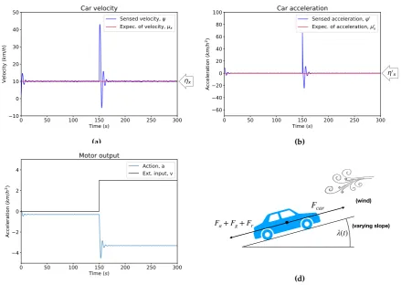
Figure 2. A cruise controller based on PI control under active inference.(a) The response of the car velocity over time with a target state, or prior in our formulation,ηx=10 km/h,ηx0=0 km/h2. (b) The acceleration of the car over time with a specified priorη0x =0 km/h2. (c) The external forcev, introduced att=150s, models a sudden change in the environmental conditions, for instance wind or change in slope. Action obtained via the minimisation of variational free energy with respect toaand counteracts the effects ofv. The motor action is never zero since we assume a constant slope,λ=4◦ (see tableA1, AppendixA). (d) The model car we implemented, wherevcould be thought as a sudden wind or a changing slope.
189
In Fig.2we show the behaviour of a standard simulation of active inference implementing PI-like
190
control for the controller of the speed of a car. The sensory and process precisionsπz,˜ πw˜ are fixed,
191
to show here only the basic disturbance rejection property of PID controllers [36,76]. In Fig.2a, after
192
the car is exposed to some new external condition (e.g. wind) represented in Fig.2cand not encoded
193
in the controller’s generative model, the regulation process brings the velocity of the car back to the 194
desired state after a short transition period. Fig.2bshows how sudden changes in the acceleration of
the car are quickly cancelled out in accord with the specified priorη0x=0 km/h2. The action of the car 196
is then shown, as one would expect [76], to counteract the external forcev, Fig.2c.
197
4.2. Responses to external and internal changes 198
It is often desirable for a PID regulator to provide different responses to external perturbations 199
(e.g. wind), which should be rather rapid, and to internal updates (e.g. a shift in target velocity) 200
which should be relatively smooth [36,45], see also section2.1. It is not, however, trivial to identify
201
and isolate parameters that contribute to these effects [37,77,78], and thus to tune these properties
202
independently. It has been suggested that in order to achieve such decoupling, a controller with two 203
degrees of freedom is necessary [45,77]. Such controller can be thought to contain a feedforward
204
model of the dynamics of the observed/regulated system [73]. In our implementation, this is elegantly
205
achieved by construction, since active inference is based on generative (forward) models. Specifically, 206
we can fix the response to external forces by setting the expected sensory precisionsπz˜(i.e. PI gains)
207
but then independently tune the response to changes in the setpoint by altering the expected process 208
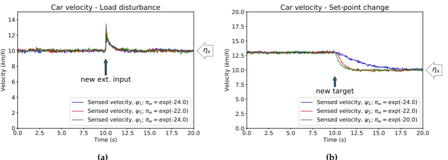
precisionsπw˜ on the priors, see Fig.3aand Fig.3b.
0.0 2.5 5.0 7.5 10.0 12.5 15.0 17.5 20.0
Time (s) 0
2 4 6 8 10 12 14
Ve
loc
ity
(k
m
/h
) x
new ext. input
Car velocity - Load disturbance
Sensed velocity, 1; w= exp(-24.0)
Sensed velocity, 1; w= exp(-22.0)
Sensed velocity, 1; w= exp(-24.0)
(a)
0.0 2.5 5.0 7.5 10.0 12.5 15.0 17.5 20.0
Time (s) 0.0
2.5 5.0 7.5 10.0 12.5 15.0 17.5 20.0
Ve
loc
ity
(k
m
/h
)
x
new target
Car velocity - Set-point change
Sensed velocity, 1; w= exp(-24.0)
Sensed velocity, 1; w= exp(-22.0)
Sensed velocity, 1; w= exp(-20.0)
(b)
Figure 3. Different responses to load disturbances and set-point changes. The simulations were 300s long, with an external disturbance/different target velocity introduced at t = 150s. Here we report only a 20 seconds time window around the change in conditions. (a) The same load disturbance (v = 3.0km/h2) is applied with varying expected process precisionsπw˜ whereπw =
{exp(−24), exp(−22), exp(−20)}. Expected sensory log-precisionsπ˜zare fixed over the duration of the simulations, withµγz = 1. (b) A similar example for changes in the target velocity of the
car, fromηx = 13km/htoηx = 10km/h, tested on varying expected process precisionsπw˜ where
πw={exp(−24), exp(−22), exp(−20)}. 209
In the limit for process prediction errors πw˜(µ˜0x+α(µ˜x−η˜x)) much larger than the sensory 210
onesπz˜(ψ˜−µ˜x)and with fixed expected sensory precisionsπz, the response to load disturbances˜
211
is invariant (Fig.3a). A new target velocity for the car creates different responses with varying
212
πw ={exp(−24), exp(−22), exp(−20)}3. Largerπw˜ values imply an expected low uncertainty on 213
the dynamics (i.e. changes to the set-point are not encoded and therefore not expected) and are met 214
almost instantaneously with an update of expected hidden states ˜µx, matched by suitable actionsa.
215
On the other hand, smallerπw˜ account for higher variance/uncertainty and thus changes in the target
216
velocity are to be expected, making the transitions to new reference values slower, as seen in Fig.3b.
217
4.3. Optimal tuning of PID gains 218
One of the main goals of modern design principles for PID controllers is to find appropriate tuning 219
rules for the gains on the prediction errors: proportional, integral and derivative terms. However, 220
existing approaches are often limited [37,38,44,48,78]. In general, the proportional term must bring a 221
system to the target state in the first place, the integral of the error should promptly deal with errors 222
generated by steady state inputs not accounted by a model [76], while the derivative term should
223
reduce the fluctuations by controlling changes in the derivative of a variable [73]. In our car example,
224
this could mean for example controlling the velocity of the vehicle in spite of changes such as the 225
presence of wind or variations in slope of the road (I term) and avoiding unnecessary changes in 226
accelerations close to the target (D term, even if sometimes not used for cruise control problems [73]).
227
In our treatment of PID controllers as approximate Bayesian inference, the controllers’ gainski,kp,kd
228
become equivalent to sensory precisionsπz,πz0,πz00, cf. equation (26) and equation (27). Following 229
[12,56,57], we thus propose to optimise these precisions to minimise the path integral of variational free 230
energy (or free action), assuming that parameters and hyperparameters change on a much slower time 231
scale. To do so, we extend our previous formulation and replace fixed sensory precisionsπz,πz0,πz00
232
withexpectedsensory precisionsµπz,µπz0,µπz00, derived from a Laplace approximation applied not only 233
to hidden statesxbut extended also to these hyperparameters, now considered as random variables to
234
be estimated, rather than fixed quantities [56,57]. 235
Active inference provides then an analytical criterion for the tuning of PID gains in the temporal domain, where otherwise mostly empirical methods or complex methods in the frequency domain
have insofar been proposed [36,38,47,48]. In frameworks used to implement active inference, such as
DEM [12,56], parameters and hyperparameters are usually assumed to be conditionally independent
of hidden states based on a strict separation of time scales (i.e. a mean-field approximation). This assumption prescribes a minimisation scheme with respect to the path-integral of free energy, or free action, requiring the explicit integration of this functional over time. In our work, however, for the purposes of building an online self-tuning controller, we will treat expected sensory precisions
as conditionally dependent but changing on a much slower time-scale with respect to states x,
using a second order online update scheme based on generalised filtering [57]. The controller gains,
µπz,µπz0,µπz00, will thus be updated specifying instantaneous changes of the curvature of expected precisions with respect to variational free energy rather than first order updates with respect to free action:
¨
µπz˜ =−
∂F
∂µπz˜
(28)
Expected precisionsµπz˜ should however be non-negative since variances need to be positive, a fact
also consistent with the negative feedback principle behind PID controllers (i.e. negative expected
precisions would apply a positive feedback). To include this constraint, following [66] we thus
parametrise sensory precisionsπz˜(and consequently expected sensory precisionsµπz˜) in the generative
model as:
πz˜=exp(γz˜) (29)
creating, effectively, log-normal priors and making them strictly positive thanks to the exponential
mapping of hyperparametersγ. The scheme in equation (28) is then replaced by one in terms of
expected sensory log-precisionsµγz˜:
¨
µγz˜ =−
∂F
∂µγz˜
For practical purposes, the second order system presented in equation (30) is usually reduced to a simpler set of first order differential equations [8]:
˙
µγz˜ =µ
0
γz˜
˙
µ0γz˜ =− ∂F
∂µγz˜
−κµ0γz˜ (31)
whereµ0γz˜ is a prior on the motion of hyperparametersγwhich encodes a “damping” term for the
minimisation of free energyF4. This term enforces hyperparameters to converge to a solution close to
the real steady state thanks to a drag term forκ>05. The parametrisation of expected precisions in
terms of log-precisionsγz, in fact, makes the derivative of the free energy with respect to log-precisions˜
strictly positive (∂F/∂γz˜ > 0), not providing a steady-state solution for the gradient descent [57]. This “damping” term stabilises the solution, reducing the inevitable oscillations around the real
equilibrium of the system. Given the free energy defined in equation (19), with exp(µγz˜)replacing
πz, the minimisation of expected sensory log-precisions (or “log- PID gains”) is prescribed by the˜ following equations:
˙
µγz =µ
0
γz
˙
µ0γz =− ∂F
∂µγz
−κµ0γz =−1
2
h
exp(µγz)(ψ−µx)
2−1i−
κµ0γz
˙
µγz0 =µ0γz0
˙
µ0γ
z0 =−
∂F
∂µγz0 −κµ0γ
z0 =− 1 2
h
exp(µγz0)(ψ 0−
µ0x)2−1 i
−κµ0γ
z0
˙
µγz00 =µ
0
γz00
˙
µ0γ
z00 =−
∂F
∂µγz00 −κµ0γ
z00 =− 1 2
h
exp(µγz00)(ψ 00−
µ00x)2−1 i
−κµ0γ
z00 (32)
This scheme introduces a new mechanism for the tuning of the gains of a PID controller, allowing 236
the controller to adapt to adverse and unexpected conditions in an optimal way, in order to avoid 237
oscillations around the target state. 238
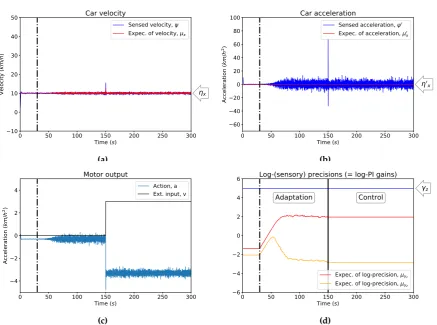
In Fig.4the controller for the car velocity is initialised with suboptimal sensory log-precisions
µγz˜, i.e. log-PI gains. The parameters were initially not updated (Fig.4d) to allow the controller to
settle around the desired state, see Fig.4a. The adaptation begins att=30s and is stopped att=150s,
when an external force is introduced, to test the response of the controller after the gains have been optimised. With the adaptation process, the controller becomes more responsive when facing external
disturbances (cf. Fig.2), quickly and effectively counteracted by prompt changes in controls, see Fig.4c.
As a trade-off, the variances of the velocity and the acceleration are however increased, see Fig.4aand
see Fig.4b. The optimisation of the gains throughµγz˜without extra constraints (if not the stopping
condition we imposed att=150s, after the adaptation reaches a steady-state) effectively introduces an
extremely responsive controller: cancelling out the effects of unwanted external inputs, such as wind in
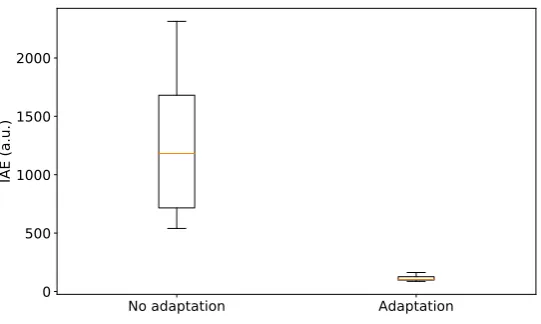
our cruise control example, but also more sensitive to measurement noise. In Fig.5we show summary
statistics with the results of the adaptation of the gains. Following the examples in Fig.2and Fig.4, we
simulated 20 different cars with expected sensory log-precisionsµγz˜ sampled uniformly in the interval
[−4,−2]and expected process log-precisionsµγw˜ in the interval[−23,−21]. We initially maintained
(i.e. no adaptation) the same hyperparameters and introduced a load disturbance att=150s, then
4 In [57] we can see that this is equivalent to the introduction of a priorp(γ˜)on the motion of ˜γto be zero (i.e. zero mean)
with precision 2κ.
0 50 100 150 200 250 300 Time (s)
10 0 10 20 30 40 50
Ve
loc
ity
(k
m
/h
)
x
Car velocity
Sensed velocity, Expec. of velocity, x
(a)
0 50 100 150 200 250 300
Time (s) 60
40 20 0 20 40 60 80 100
Ac
ce
ler
at
ion
(k
m
/h
2)
0x
Car acceleration
Sensed acceleration, 0
Expec. of acceleration, x0
(b)
0 50 100 150 200 250 300
Time (s) 4
2 0 2 4
Ac
ce
ler
at
ion
(k
m
/h
2)
Motor output
Action, a Ext. input, v
(c)
0 50 100 150 200 250 300
Time (s) 6
4 2 0 2 4 6
z
Adaptation
Control
Log-(sensory) precisions (= log-PI gains)
Expec. of log-precision, z
Expec. of log-precision, z0
(d)
Figure 4. Optimising PID gains as expected sensory log-precisionsµγz˜. This example shows the
control of the car velocity before and after the optimisation ofµγz˜(before and after the vertical dash
dot black line) is introduced. (a) The velocity of the car. (b) The acceleration of the car. (c) The action of the car, with an external disturbance introduced att=150s. (d) The optimisation of expected sensory precisionsµγz˜and their convergence to an equilibrium state, after which the optimisation is stopped
before introducing an external force. The blue line represents the true log-precision of observation noise in the system,γz=γz0=5.
repeated the simulations (20 cars) with the same initial conditions allowing for the adaptation of
expected sensory log-precisions as log-PI gains aftert=30s, as in Fig.4. Following [79], we measured
the performance of the controllers by defining the integral absolute error (IAE):
I AE=
Z t+τ
t |e
(t)| dt (33)
between two zero-crossings: the last time the velocity was at the target value before a disturbance is 239
introduced, assumed to bet=150 in our case, and the first time the velocity goes back to the target
240
after a disturbance is introduced (t+τ). To computet+τ, we took into account the stochasticity of
241
the system and errors due to numerical approximations, considering the case for the real velocity to be 242
within a±0.5 km/h interval away from the target value. The IAE captures the impact of oscillations
243
on the regulation problem by integrating the error over the temporal interval where the car is pushed 244
away from its target due to some disturbance (for more general discussions on its role and uses see 245
[36]). As we can see in Fig.5, the IAE converges to a single value for all cars (taking into account our
246
approximation of a±0.5 km/h interval while measuring it) and is clearly lower when the adaptation
247
mechanism for expected sensory log-precisions is introduced, making the controller very responsive 248
to external forces and thus reducing the time away from the target velocity, see Fig.4for an example.
No adaptation
Adaptation
0
500
1000
1500
2000
IAE (a.u.)
Figure 5. Performance of PID controllers with and without adaptation of the gains based on the minimisation of free energy.The integral absolute error (IAE) is used to measure the effects of the oscillations introduced by a single load disturbance att=150s (see text for the exact definition of the IAE).
5. Discussion 250
In this work we developed a minimal account of regulation and control mechanisms based on 251
active inference, a process theory for perception, action and higher order functions expressed via 252
the minimisation of variational free energy [4,8,10,13]. Our implementation constitutes an example
253
of the parsimonious, action-oriented models described in [24,25], connecting them to methods from
254
classic control theory. We focused in particular on Proportional-Integral-Derivative (PID) control, both 255
extensively used in industry [36–38,78] and more recently emerging as a model of robust feedback
256
mechanisms in biology, implemented for instance by bacteria [39], amoeba [40] and gene networks
257
[41], and in psychology [42]. PID controllers are ubiquitous in engineering mostly due to the fact that
258
one needs only little knowledge of the process to regulate. In the biological sciences, this mechanism is 259
thought to be easily implemented even at a molecular level [43] and to constitute a possible account
260
for limited knowledge of the external world in simple agents [76].
261
Following our previous work on minimal generative models [26], we showed that this mechanism
262
corresponds, in active inference terms, to linear generative models for agents that only approximate 263
properties of the world dynamics. Specifically, our model describes linear dynamics for a single 264
hidden or latent state and a linear mapping from the hidden state to an observed variable, representing 265
knowledge of the world that is potentially far removed from the real complexity behind observations 266
and their hidden variables. To implement such model, we defined a generative model that only 267
approximates the environment of an agent and showed how under a set of assumptions including 268
analytic (i.e. non-Markovian, differentiable) Gaussian noise and linear dynamics, this recapitulates PID 269
control. A crucial component of our formulation is the presence of low sensory precision parameters on 270
proprioceptive prediction errors of our free energy function or equivalently, high expected variance of 271
proprioceptive signals. These low precisions play two roles during the minimisation of free energy: (1) 272
they implement control signals as predictions of proprioceptive input influenced by strong priors (i.e. 273
desires) rather than by observations, see equation (24) and [13], and (2) they reflect a belief that there
274
are large exogenous fluctuations (low precision = high variance) in the observed proprioceptive input. 275
This last point can be seen as the well known property of the Integral term [73,76] of PID controllers,
276
dealing with unexpected external input (i.e. large exogenous fluctuations). The model represented by 277
derivatives∂ψ˜/∂aencodes then how actionsaapproximately affect observed proprioceptive sensations
278 ˜
ψ, with an agent implementing a sensorimotor mapping that does not match the real dynamics of
279
actions applied to the environment. The formulation in equation (20) and equation (21) can in general
be applied to different tasks, in the same way PID control is used in different problems without specific 281
knowledge of the system to regulate. 282
The generative model we used is expressed in generalised coordinates of motion, a mathematical 283
construct used to build non-Markovian continuous stochastic models based on Stratonovich calculus. 284
Their importance has been expressed before [12,56,57], for the treatment of real world processes
285
best approximated by continuous models and for which Markov assumptions don’t really hold (see 286
also [69] for discussion). The definition of ageneralisedstate-space model provides then a series of
287
weighted prediction errors and their higher orders of motion from the start, with PID control emerging 288
as the consequence of an agent trying to impose its desired prior dynamics on the world via the 289
approximate control of its observations on different embedding orders (for I, P and D terms). In 290
this light, the ubiquitous efficacy of PID control may thus reflect the fact that the simplest models of 291
controlled dynamics are first-order approximations to generalised motion. This simplicity is mandated 292
because the minimisation of free energy is equivalent to the maximisation of model evidence, which 293
can be expressed as accuracy minus complexity [10,24]. On this view, PID control emerges via the
294
implementation of constrained (parsimonious, minimum complexity) generative models that are, 295
under some constraints, the most effective (maximum accuracy) for a task. 296
In the control theory literature, many tuning rules for PID gains have been proposed (e.g. 297
Ziegler-Nichols, IMC, etc., see [36,38] for a review) and used in different applications [36–38,48,78], 298
however most of them produce quite different results, highlighting their inherent fit to only one of 299
many different goals of the control problem. With our active inference formulation, we argue that 300
different criteria can and should be expressed within the same set of equations in order to better 301
understand their implications for a system. Modern approaches to the study of PID controllers propose 302
four points as fundamental features to be considered for the design of a controller [44]:
303
• load disturbance response
304
• set-point response
305
• measurement noise response
306
• robustness to model uncertainty.
307
In our formulation, these criteria can be interpreted using precision (inverse variance) parameters of 308
different prediction errors in the variational free energy, expressing the the uncertainty associated to 309
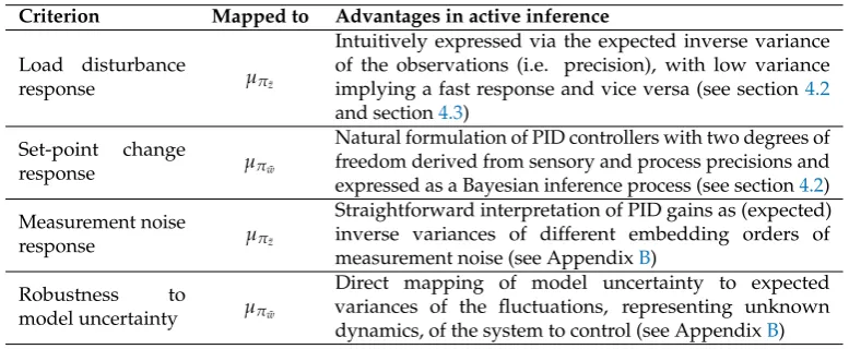
observations and priors, as reported in table1, see also AppendixBfor further reference.
Table 1. Active inference as a general framework for PID controllers.
Criterion Mapped to Advantages in active inference
Load disturbance
response µπz˜
Intuitively expressed via the expected inverse variance of the observations (i.e. precision), with low variance implying a fast response and vice versa (see section4.2
and section4.3)
Set-point change
response µπw˜
Natural formulation of PID controllers with two degrees of freedom derived from sensory and process precisions and expressed as a Bayesian inference process (see section4.2)
Measurement noise
response µπz˜
Straightforward interpretation of PID gains as (expected) inverse variances of different embedding orders of measurement noise (see AppendixB)
Robustness to
model uncertainty µπw˜
Direct mapping of model uncertainty to expected variances of the fluctuations, representing unknown dynamics, of the system to control (see AppendixB)
310
After establishing the equivalence between PID control and linear approximations of generalised 311
motion in generative models, we showed that the controllers’ gains,ki,kp,kd, are in our formulation
312
equivalent to expected precisions,µπz,µπz0,µπz00, for which a minimisation scheme is provided in
313
[12,56,57]. The basic version of this optimisation produces also promising results in presence of
314
time-varying measurement (white) noise in the simulated car (see Fig.A1 in AppendixB). If the
![Figure 1. A PID controller [46]. The prediction error e(t) is given by the difference between a referencesignal r(t), yr in our formulation, and the output y(t) of a process](https://thumb-us.123doks.com/thumbv2/123dok_us/8023251.1334617/4.595.121.477.110.240/figure-controller-prediction-difference-referencesignal-formulation-output-process.webp)