University of South Carolina
Scholar Commons
Theses and Dissertations
2018
Semiparametric Statistical Estimation and
Inference with Latent Information
Qianqian Wang
University of South CarolinaFollow this and additional works at:https://scholarcommons.sc.edu/etd Part of theStatistics and Probability Commons
This Open Access Dissertation is brought to you by Scholar Commons. It has been accepted for inclusion in Theses and Dissertations by an authorized administrator of Scholar Commons. For more information, please [email protected].
Recommended Citation
Wang, Q.(2018).Semiparametric Statistical Estimation and Inference with Latent Information.(Doctoral dissertation). Retrieved from
Semiparametric Statistical Estimation and Inference with Latent Information
by
Qianqian Wang
Bachelor of Science Lanzhou University 2011
Master of Science
Michigan State University 2013
Submitted in Partial Fulfillment of the Requirements
for the Degree of Doctor of Philosophy in
Statistics
College of Arts and Sciences
University of South Carolina
2018
Accepted by:
Yanyuan Ma, Major Professor
John Grego, Committe Member
Yen-Yi Ho, Committe Member
Lianming Wang, Committee Member
c
Acknowledgments
I own a sincere thank you to professor Yanyuan Ma, for being my research advisor
and for spending countless of hours discussing research work with me and encouraging
me throughout my PhD study. I would like to thank professor John Grego, Yen-Yi
Ho and Lianming Wang for being my committee members and for their guidance
and support. I would like to thank professor Guangren Yang and Xia Cui for their
collaboration of my research project. I would especially like to thank my family and
Abstract
In Chapter 1, we predicted disease risk by transformation models in the presence of
missing subgroup identifiers. When a discrete covariate defining subgroup
member-ship is missing for some of the subjects in a study, the distribution of the outcome
follows a mixture distribution of the subgroup-specific distributions. Taking into
account the uncertain distribution of the group membership and the covariates, we
model the relation between the disease onset time and the covariates through
trans-formation models in each sub-population, and develop a nonparametric maximum
likelihood based estimation implemented through EM algorithm along with its
in-ference procedure. We further propose methods to identify the covariates that have
different effects or common effects in distinct populations, which enables
parsimo-nious modeling and better understanding of the difference across populations. The
methods are illustrated through extensive simulation studies and a real data example.
In Chapter 2, we discussed a generalized partially linear single index model with
measurement error, instruments and binary response. Instrumental variables are
im-portant elements in studying many errors-in-variables problems. We use the relation
between the unobservable variables and the instruments to devise consistent
estima-tors for partially linear generalized single index models with binary response. We
establish the consistency, asymptotic normality of the estimator and illustrate the
numerical performance of the method through simulation studies and a data
exam-ple. Despite the connection to Xu et al. (2015) in its general layout, the mathematical
derivations are much more challenging in the context studied here.
par-tially linear model. Different from the usual literature (Ma & Carroll 2006), we
consider the case where the measurement error occurs to the covariate that enters
the model nonparametrically, while the covariates precisely observed enter the model
parametrically. To avoid the deconvolution type operations, which can suffer from
very low convergence rate, we use the B-splines representation to approximate the
nonparametric function and convert the problem into a parametric form for
opera-tional purpose. We then use a parametric working model to replace the distribution
of the unobservable variable, and devise an estimating equation to estimate both
the model parameters and the functional dependence of the response on the latent
variable. The estimation procedure is devised under the functional model framework
without assuming any distribution structure of the latent variable. We further
de-rive theories on the large sample properties of our estimator. Numerical simulation
studies are carried out to evaluate the finite sample performance, and the practical
Table of Contents
Acknowledgments . . . iii
Abstract . . . iv
List of Tables . . . viii
List of Figures . . . ix
Chapter 1 Predicting disease Risk by Transformation Models in the Presence of Missing Subgroup Identifiers . . . 1
1.1 Introduction . . . 1
1.2 Modeling, Estimation, and Asymptotic Properties . . . 3
1.3 Homogeneous and no covariate effect model . . . 11
1.4 Simulation Studies . . . 13
1.5 Application to Huntington’s Disease Study . . . 15
1.6 Discussion . . . 17
Chapter 2 Generalized Partially Linear Single Index Model with Measurement Error, Instruments and Binary Response . . . 22
2.1 Introduction . . . 22
2.2 Estimation procedure via profiling and the asymptotic properties . . 24
2.4 Real data analysis . . . 32
2.5 Discussion . . . 33
Chapter 3 Locally efficient estimation in generalized par-tially linear model with measurement error in non-linear function . . . 35
3.1 Introduction . . . 35
3.2 Main results . . . 37
3.3 Asymptotic properties . . . 43
3.4 Numerical Study . . . 45
3.5 Data Analysis . . . 47
3.6 Discussion . . . 48
Bibliography . . . 50
Appendix A Permission to Reprint . . . 54
Appendix B Chapter 1 Appendix . . . 55
Appendix C Chapter 2 Appendix . . . 60
List of Tables
Table 1.1 Simulation results based on 1000 repetitions. . . 19
Table 1.2 COHORT analysis results: estimated covariate effects (age, gen-der, proband’s diagnosis of HD), their standard errors, andp-values. 19 Table B.1 Simulation results. Results based on 1000 simulations. . . 58
Table C.1 Simulation 1 results (link function: logit) . . . 70
Table C.2 Simulation 2 results (link function: logit) . . . 72
Table C.3 Simulation 3 results (link function: logit) . . . 73
Table C.4 Simulation 1 results (link function: probit) . . . 74
Table C.5 Simulation 2 results (link function: probit) . . . 75
Table C.6 Simulation 3 results (link function: probit) . . . 76
Table C.7 Realdata analysis results . . . 76
Table D.1 Simulation results under a correct working model . . . 83
Table D.2 Simulation results under a misspecified working model . . . 83
List of Figures
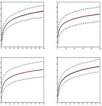
Figure 1.1 True function (solid line), median estimation (dashed line), mean estimation (dotted line) and 95% confidence band (dash-dotted line) ofH(T) in simulations 1.1 left), 1.2
(upper-right), 2 (lower-left), and 3 (lower-right) . . . 20
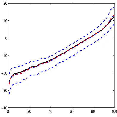
Figure 1.2 Estimated H function (solid line), median estimation (dashed line), mean estimation (dash-dotted line) and 95% confidence band (dashed line) ofH(T) in data analysis. Median, mean and
95% confidence band are based on 1000 bootstrapped samples. . 21
Figure 1.3 Fitted linear function Hc(t) versus aget for HD data analysis. . . 21
Figure B.1 True function (solid line), median estimation (dashed line), mean estimation (dotted line) and 95% confidence band (dash-dotted line) of H(T) in simulations 4 left), 5
(upper-right), and 6 (lower) . . . 59
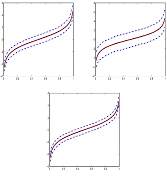
Figure C.1 True function (black line), median estimation (gree line), mean estimation (red line) and 95% confidence band (blue line) of
g(u) in simulations 1 (upper-left), 2 (upper-right) and 3 (lower) when link function is inverse logit, is normal distributed and
with OLS method applied. . . 71
Figure C.2 Plot of averaged baseline CD4 count versus screening CD4 count. 72
Figure C.3 Estimated g(u) for real data (black line), median estimation (green line), mean estimation (red line) and 90% confidence
band (blue line) ofg(u) using 1000 bootstrapped samples . . . . 77
Figure D.1 True function (black line), median estimation (green line), mean estimation (red line) and 90% confidence band (blue line) of
g(x) in simulation 1. Correct working model on the left and
Figure D.2 True function (black line), median estimation (green line), mean estimation (red line) and 90% confidence band (blue line) of
g(x) in simulation 2. Correct working model on the left and
misspecified working model on the right. . . 84
Figure D.3 Estimated g(x) for real data (black line), median estimation (green line), mean estimation (red line) and 90% confidence
Chapter 1
Predicting disease Risk by Transformation
Models in the Presence of Missing Subgroup
Identifiers
11.1 Introduction
Biomedical studies can lead to mixture data. When a discrete covariate defining
subgroup membership is missing for some of the subjects in a study, the distribution
of the outcome is a mixture of the subgroup-specific distributions. One example is the
kin-cohort study Wacholder et al. (1998) with the goal of estimating the cumulative
risk of disease for mutation carriers Khoury et al. (1993). However, mutation status
is only collected in the initial sample of participants, referred as probands, not in
their relatives. For example, genetic mutation status is not available for deceased
relatives or those who have not undergone genetic testing due to resource constraints.
The disease phenotype information for such relatives is available from other sources,
such as interviewing the proband in a family Marder et al. (2003). For a late-onset
disease, such as Parkinson’s disease (PD), parents of study participants are often
deceased. Therefore even though age-at-onset of PD is provided by a family member,
no genotyping can be performed on deceased parents. When estimating the disease
risk distribution for mutation carriers and non-carriers using these relatives’ disease
onset information, the unknown mutation status needs to be accounted for by using
1Wang Q., Ma, Y., and Wang, Y. 2017. Statistica Sinica. 27, 4, p. 1857-1878 22 p.
the distribution of mutation status in such relatives as estimated from living relatives
who provide blood sample Wang et al. (2012), Ma & Wang (2014).
We consider estimating the subgroup-specific distribution for outcomes that are
subject to censoring and with missing subgroup identifiers. The nonparametric
mod-els in Wacholder et al. (1998), Wang et al. (2012), and Ma & Wang (2014) do not
include any covariates other than the mutation status. We consider how to include
covariates that can have identical or different effects across subgroups. Popular
semi-parametric models for censored outcomes, such as the Cox proportional hazards
model, accelerated failure time model, and transformation model have been
stud-ied extensively in the literature, but less so in a mixture data setting. Recently,
Altstein & Li (2013) proposed a latent subgroup analysis for a semiparametric
accel-erated failure time model in a clinical trials setting. Our work differs from Altstein
& Li (2013) in that the distribution of the subgroup identifiers is available in our
problem, and we assume a semiparametric transformation model in each subgroup.
A transformation model is applied to analyze neurological disorder data (e.g,
Hunt-ington’s disease [HD] as in our motivating study) due to its useful biological and
clinical interpretations; see for example Zhang et al. (2012).
We propose a semiparametric transformation model for mixture data. Compared
to parametric transformation model in the literature Zhang et al. (2012), we allow
for greater flexibility to account for subgroup heterogeneity. This is achieved in our
model through characterizing the outcome in each subpopulation using a different
distribution, indexed by both parameters and error distributions. They can also have
both as shared covariate effect and/or a subgroup-specific covariate effect. In
addi-tion, we assume an unknown transformation to avoid the difficulty of specifying a
parametric transformation. When assuming a homogeneous covariate effect, we
ac-count for a missing population identifier by taking advantage of the distribution of the
simplifies the procedure. When we assume a subgroup-specific covariate effect, the
weighted least-square estimator no longer applies, and we use the EM algorithm. We
have performed extensive simulation studies to examine performance of the proposed
approach and applied it to estimating the survival function for HD mutation
carri-ers in a large genetic epidemiology study Dorsey & The Huntington Study Group
COHORT Investigators (2012).
1.2 Modeling, Estimation, and Asymptotic Properties
Assume there are n observations from p populations. Here p is usually determined
by the research purpose. For genetic studies, populations are defined by mutation
carrier status. Throughout, we assume p is pre-determined. Denote the data from
the ith observation as Oi = (qi,xi,zi, yi, δi), where qi is a length p vector, with the
jth entryqij being the probability that the ith observation is randomly sampled from
the jth population. We also allow a subject’s population membership to be known
by allowingqi to be a vector with 1 in one component and zero in all others. Let ti
be the time to event andci be the censoring time, yi = min(ti, ci), andδi =I(ti ≤ci).
Letxi denote the covariate vector that has a common effect on the event time across
different populations, while zi denotes the covariate vector that has a different effect
in different populations. For simplicity, we sort the data so thatyi ≤yk for all i < k.
1.2.1 Model
For the jth population, the linear transformation model we propose has the form
H(T) =−XTβ−ZTαj+j. (1.1)
Here H is an unknown, monotonically increasing function and, without loss of
gen-erality, we assume H(0) = −∞. We assume j is independent of X, Z, and has
classical linear transformation model, in which the baseline population distribution
can be heterogeneous due to the different choices of fj. Selection of fj for each
pop-ulation can be based on scientific or biological knowledge of a particular poppop-ulation.
The covariate effect is also allowed to vary, reflected in the population-specificαj. By
including the termxTβ, we also allow the possibility that some covariates have a
ho-mogeneous effect across populations. We develop a test to assess whether a covariate
exhibits evidence of deviation from a homogeneous effect model.
Let θ = (βT,αT1, . . . ,αTp)T, Φ(t) = exp{H(t)}, and φ(t) = exp{H(t)}h(t). The
conditional distribution function of theith relative from (1.1) is then
f(yi, δi |xi,zi;θ,Φ, φ)
=
h(yi) n X
j=1
qijfj{H(yi) +xTi β+z
T
i αj}
δi
×
1− n X
j=1
qijFj{H(yi) +xTi β+z
T
i αj}
1−δi
= φ(yi)δiΨ(Oi;θ,Φ),
where Φ is a function that depends only on θ and Φ, but not on φ. The model can
not be viewed as a transformation model, hence existing estimation procedures do
not apply. To ensure identifiability, we require that the qi variable takes m different
vector values, denoted u1, . . . ,um, so that the matrix (u1, . . . ,um) has rank p. We
point out that the identifiability here excludes any permutation. This identifiability
is stronger than that up to a permutation in most classical mixture models Holzmann
et al. (2006). We can achieve the stronger form of identifiability because the mixture
1.2.2 Estimation
We propose a nonparametric maximum likelihood estimator (NPMLE) to estimateθ
and Φ(·). Specifically, we obtain θb and Hc= log(Φ) through maximizingb
l(θ,Φ) = n X
i=1
δilog{φ(yi)}+ n X
i=1
log{Ψ(Oi;θ,Φ)}
with respect to θ and Φ, where we restrict Φ, hence H, to be a piecewise constant
non-decreasing function with non-negative jumps only at the observed event times.
Following existing literature Wacholder et al. (1998), Wang et al. (2012), We exclude
the probands from the analysis sample and the likelihood to protect against
poten-tial ascertainment bias from unknown sources that may be difficult to adjust (e.g.,
convenience sample of patients visiting a clinic). Given the mutation carrier status,
we also assume the relatives’ phenotypes are conditionally independent of probands’
phenotypes, which is an assumption satisfied by a monogenic disorder with a known
genetic cause controlled in the model (e.g., HD in our application).
Although conceptually simple, the computation of NPMLE is not straightforward
because the maximization is with respect to not only γ, but also Φ(·) at all the yi’s
that are not censored. As sample size increases, the potential number of parameters
increases as well, hence the computational problem does not simplify in the
asymp-totic sense. To overcome the computational difficulty, we use an EM algorithm. To
this end, we first use Laplace transformation in each population to obtain
1−Fj(x) = Z ∞
0
exp(−rjex)ψj(rj)drj,
consequently
1−
n X
j=1
qijFj{H(yi) +xTi β+z
T
i αj}
= n X j=1 qij Z ∞ 0
exp{−rijeH(yi)+x
T
iβ+z
T
iαj}ψ
j(rij)drij
= n X j=1 qij Z ∞ 0
exp{−rijΦ(yi)ex
T
iβ+zTiαj}ψ
j(rij)drij
and
h(yi) n X
j=1
qijfj{H(yi) +xTi β+zTi αj}
= n X j=1 qij Z ∞ 0
exp{−rijΦ(yi)ex
T
iβ+z
T
iαj}φ(yi) exp(xT i β+z
T
i αj)rijψj(rij)drij.
The ith observation here is Oi, let D = (O1,· · · ,On). Let 0 < t1 < · · · <
tK < τ be the distinct event times, and write the quantities to be estimated as
γ = {θT, H(t1), . . . H(tK)}T. The log-likelihood is then l(γ;D) = Pni=1li(γ;Oi),
where
li(γ;Oi) = log n X
j=1
Z ∞
0
{φ(yi)rijexp(xTi β+z
T
i αj)}δi
×exp{−rijΦ(yi)ex
T
iβ+z
T
iαj}q
ijψj(rij)drij.
We take advantage of this special data structure and view the population identifiers
G = (G1, . . . , Gn) and r = (r1, . . . ,rn) as the missing variable, where Gi = Ij
rep-resents that the ith observation is a random sample from the jth population, and
ri = (ri1, . . . , rip)T is the introduced random effects to facilitate computation. Then
the complete data loglikelihood isl(γ |D,G,r) =Pn
i=1li(γ |Oi, Gi,ri), where
li(γ|Oi, Gi =Ij, rij)
= logh{φ(yi)rijexp(xTi β+z
T
i αj)}δiexp{−rijΦ(yi)ex
T
iβ+zTiαj}i
This is a Cox model log-likelihood. Thus, in the E-step, we calculate
Q(γ,γ(u),D)≡Eγ(u){l(γ |D,G,r)|D}=
n X
i=1
R Pn
j=1li(γ|Oi,Gi =Ij, rij)a(iju)drij R Pn
j=1a (u)
ij drij
,
where
a(iju) ={φ(u)(yi)rijexp(xTi β
(u)
+zTi α(ju))}δiexp{−rijΦ(u)(yi)ex
T
iβ
(u)+zT
iα
(u)
j }q
ijψj(rij).
In the M-step, we maximizeQ(γ,γ(u),D) with respect toγsubject to the constraints
0 < H(t1) < · · · < H(tK) ≤ 1 to obtain γ(u+1). Specifically, taking derivative with
respect toγ, we obtain estimating equations
0 =
n X
i=1
R Pn
j=1{δixi−xirijΦ(yi)ex
T
iβ+z
T
iαj}a(u) ij drij
R Pn j=1a
(u)
ij drij
= n X
i=1
δixi−xiΦ(yi)ex
T
iβ Pn
j=1ez T
iαjR rija(u) ij drij
R Pn j=1a
(u)
ij drij
.
Forj = 1, . . . , p,
0 =
n X
i=1
R
(δizi−zirijeH(yi)+x
T
iβ+z
T
iαj)a(u) ij drij
R Pn j=1a
(u)
ij drij
= n X
i=1 δizi
R
a(iju)drij−ziΦ(yi)ex
T
iβ+zTiαjR r ija
(u)
ij drij
R Pn j=1a
(u)
ij drij
.
Fork = 1, . . . , K,
0 = X
yi≥tk R Pn
j=1
nI(yi=tk) φk −rije
xT
iβ+zTiαjoa(u) ij drij
R Pn j=1a
(u)
ij drij
= 1
φk
− X
yi≥tk
exTiβPn j=1ez
T
iαjR
rija(iju)drij
R Pn j=1a
(u)
ij drij
.
This yields
φk=
X
yi≥tk
exTiβPn j=1ez
T
iαjR rija(u) ij drij
R Pn j=1a
(u)
ij drij
−1
,
or in general
φ(yk;β,α) = δk
n X
i=1
I(yi ≥yk)ex
T
iβPn j=1ez
T
iαjR r ija
(u)
ij drij
R Pn j=1a
(u)
ij drij
−1
(1.2)
Φ(yi;β,α) = n X
k=1
I(yk ≤yi)δk
n X
i=1
I(yi ≥yk)ex
T
iβPn j=1ez
T
iαjRr ija
(u)
ij drij
R Pn j=1a
(u)
ij drij
−1
Plugging into the estimating equation for β,α1, . . . ,αp, we obtain
n X
i=1
δixi−xiΦ(yi;β,α)ex
T
iβ Pn
j=1ez T
iαjR r ija
(u)
ij drij
R Pn j=1a
(u)
ij drij
= 0 (1.3)
n X
i=1 δizi
R
a(iju)drij−ziΦ(yi;β,α)ex
T
iβ+zTiαjR r ija
(u)
ij drij
R Pn j=1a
(u)
ij drij
= 0
atj = 1, . . . , p.
We solve the estimating equations (1.3) to obtainβb
(u+1) ,αb
(u+1)
, j = 1, . . . , p, and
then substitute into (1.2) to obtain Φ(u+1)(t), and hence alsoH(u+1)(t) = log{Φ(u+1)(t)}.
The procedure iterates between the E-step and the M-step until convergence.
We point out that, although the functions ψj(r)’s are left as unknown, we can
still calculateR
a(iju)drij and R
rija
(u)
ij drij in the M-step. Specifically,
Z
a(iju)drij
= qij{1−Fj(t)}1
−δin
h(u)(yi)fj(t) oδi
t=H(u)(yi)+xT
iβ
(u)+zT
iα
(u)
j
,
Z
rija( u)
ij drij
= ne−tqijfj(t) o1−δh
e−tqijh(u)(yi){fj(t)−fj0(t)} iδ
t=H(u)(yi)+xT
iβ(u)+zTiα
(u)
j
,
as shown in Appendix B.1, by taking advantage of the Laplace/inverse Laplace
trans-form relation. In fact, even if an explicit trans-form ofψj(r) can be obtained, it is not
neces-sary to go through the calculation becauseψj(r) itself is not needed. Finally, because
ψj is defined as the inverse Laplace transform of a bounded function, it always exists
for any distribution.
1.2.3 Theoretical properties
Although (1.1) is not a transformation model, under the list of conditions imposed
in Appendix B.2, it can be cast into the general framework, Zeng & Lin (2007). To
this end, we can verify that our Conditions (a), (b), (c) lead to their conditions (C1),
(C4) and (C8). Our Condition (f) leads to their condition (C6), and our Condition
(g) leads to their conditions (C5), (C7). These are mild conditions mainly imposing
identifiability, sufficient smoothness, and boundedness of various functions; They are
usually satisfied in practice. Having verified the regularity conditions C1-C7 of Zeng
& Lin (2007), we can use their results to obtain the asymptotic properties of the
NPMLE in the linear transformation model in the mixture data setting. We state
the results in Theorem 1 and provide the proof in Appendix B.3.
Theorem 1. Letθ0,Φ0denote the true value ofθ,Φ, and writeΦ ={Φ(t1),Φ(t2), . . . ,
Φ(tK)}T. Under conditions (a)-(g) of Appendix B.2,θb,Φb are consistent, and have the
asymptotic property that √n(θb−θ,Φb−Φ)converges weakly to a zero mean Gaussian
process. Then, for any functiona1(s)with bounded total variation and any vector a2, √
nR
a1(s)d{Φ(b s)−Φ(s)}+
√ naT
2(θb−θ)converges to a zero mean normal distribution
whose variance can be approximated by
v{a1(·),a2} ≡ −(aT1,a T
2)
(
∂2l(Φb,θb) ∂(ΦT,θT)∂(ΦT,θT)T
)−1
(aT1,aT2)T,
where a1 ={a1(t1), . . . , a1(tK)}T.
1.2.4 Inference
The main interest is often in the covariate effects described by θ. In such cases, we
can perform inference using the results of a profiling procedure: at any θ, we use
the same EM algorithm to calculate Hc(T,θ) except that we hold θ fixed, and then
calculate the information matrix using numerical derivatives. This is a simplification
example, the α100% confidence interval for the jth component of θ, θj is
b
θj±Z(1+α)/2
"
−
n X
i=1 ∂2l
i{θ,Hc(t1,θ), . . . ,Hc(tK,θ)}
∂θ2 j θ= b θ
#−1/2
≈ θbj±Z(1+α)/2 " n
X
i=1
−li{θb +bej,Hc(t1,θb+bej), . . . ,Hc(tK,θb+bej)}
b2
+2li{θb,Hc(t1,θb), . . . ,Hc(tK,θb)}
b2
−li{θb −bej,Hc(t1,θb −bej), . . . ,Hc(tK,θb −bej)} b2
#−1/2
,
where Z(1+α)/2 is the (1 +α)/2 quantile of the standard normal distribution, li is
the likelihood evaluated at theith observation, ej is the vector with zero components
everywhere except thejth component being 1, andbis a small number that facilitates
the numerical derivative.
Likewise, for hypothesis testing of the form H0 :θ =c, we can construct the test
statistic Z = " − n X i=1
∂2li{θ,Hc(t1,θ), . . . ,Hc(tK,θ)}
∂θ∂θT
θ=
bθ #1/2
(θ−c)
≈
" n X
i=1
−li{θb+bej+bek,Hc(t1,θb +bej +bek), . . . ,Hc(tK,θb +bej +bek)}
4b2
+li{θb +bej −bek,Hc(t1,θb +bej −bek), . . . ,Hc(tK,θb +bej −bek)} 4b2
+li{θb −bej+bek,Hc(t1,θb −bej +bek), . . . ,Hc(tK,θb −bej +bek)} 4b2
−li{θb −bej −bek,Hc(t1,θb −bej −bek), . . . ,Hc(tK,θb−bej−bek)}
4b2
!
jk
1/2
×(θ−c),
and note that Z is approximately a standard multivariate normal random variable
under H0. Here, we use the notation (Ajk) to denote the square matrix A with size
1.3 Homogeneous and no covariate effect model
When either β or αj does not appear in (1.1), the model is more restrictive and the
computation simplifies. Ifβdoes not appear, then there is no homogeneous covariate
effect in the transformation model. In terms of estimation, the procedures follows
the same line with some minor simplifications. However, if αj does not appear, (1.1)
greatly simplifies and can be treated quite differently, as we now explain.
The common-effect covariate effect model for the jth population is
H(T) = −XTβ+j,
where all the components in the model retain the same interpretation as in (1.1). The
implication of the model is that the heterogeneity between subpopulations is due to
the different variability of measurement errors, but not the heterogeneous effect of
covariates. The conditional distribution is then simplified to
f(Y,∆|X) =
h(y) n X
j=1
qjfj{H(y) +xTβ}
δ
1− n X
j=1
qjFj{H(y) +xTβ}
1−δ
= hh(y)qTf{H(y) +xTβ}iδh1−qTFnH(y) +xTβoi1−δ,
where f = (f1, . . . , fp)T, F = (F1, . . . , Fp)T, and h(y) ≡ H0(y), because the same
transformation H and the same parameter β are assumed across all p populations.
The population difference is only reflected in the distribution ofj, which is assumed
to be fj. We can however still use the different fj’s of the model to account for
unexplained residual population heterogeneity, for example, different variances.
As before, estimating the distribution in each population is equivalent to
estimat-ing H and β. As the qi’s have m ≥ p different vector values u1, . . . ,um, assign the
n observations to these m groups according to their q values. Assume there are,
re-spectively,r1, . . . , rm observations in each group. In group k, we can view the model
as a transformation model with the same transformation H, the same parameter β,
but a new distribution for , which has the mixture form uT
the existing estimation method for transformation models to obtain the estimators
of H and β, using exclusively the kth group data. Denote the resulting estimators
as Hck and βb
k. We can then take the weighted average to obtain the final estimator
c
H(t) = Pm
k=1wk(t)Hck(t) and βb =Pm
k=1wkβbk. To be consistent with the estimation
in the general model (1.1), we use the NPMLE proposed by Zeng & Lin (2006). Thus,
we obtainβbk, Hck via maximizing
lk(H,β) = n−1 n X
i=1
I(qi =uk)
δilog h
h(yi)uTkf{H(yi) +xTi β} i
+(1−δi)log h
1−uTkFnH(yi) +xTi β oi
with respect to β and H. Here, we restrict H(y) to be a piecewise constant
non-decreasing function with nonnegative jumps only at the yi’s where qi = uk and
δi = 1. We write these jump points t1, . . . , tK, and write Hk ={H(t1), . . . , H(tK)}T.
Zeng & Lin (2006) showed that the resultingβbk,Hckare consistent, and that
√
n(βbk−
β,Hck−H) converges weakly to a zero mean Gaussian process. Thus, for any function
a1(s) with bounded total variation and any vector a2, √
nR
a1(s)d{Hck(s)−H(s)}+
√
naT2(βbk−β) converges to a zero mean normal distribution whose variance can be
approximated by
vk{a1(·),a2} ≡ −(aT1,aT2)
(
∂2lk(Hck,βb k)
∂(HTk,βT)∂(HTk,βT)T
)−1
(aT1,aT2)T,
where a1 ={a1(t1), . . . , a1(tK)}T.
It remains to determine the choice of weights wk. Because the estimation in
different group is based on different subjects, they are independent. Hence the optimal
weights are proportional to the inverse of the variance of the estimators. The optimal
weights forHc(t) are thenwk(t) = vk{I(s≤t),0}−1/[Pm
k=1vk{I(s≤t),0}−1]. wkis a
diagonal matrix with the jth diagonal elementwkj =vk(0,ej)−1/{Pmk=1vk(0,ej)−1}.
In practice, this may not work well since it relies on asymptotic results. Based on
prior work in Ma & Wang (2014), a simple choice ofwk(t) = wk =r−k1has satisfactory
Because the within group NPMLE already guarantees the monotonicity of each
c
Hk, the final weighted average estimator forHcis monotone. The asymptotic property
ofHcandβis standard:
√
n(βb−β,Hc−H) converges weakly to a zero mean Gaussian
process. Then, for any function a1(t) with bounded total variation and any vector
a2, √
nR
a1(s)d{Hc(s)− H(s)}+
√ naT
2(βb − β) converges to a zero mean normal
distribution whose variance can be approximated with
v{a1(·),a2} ≡
m X
k=1
vk{a1(·)wk(·),wka2}
where t1, . . . , tK are the observed event times.
Testing whether population heterogeneity in the covariate effects is present in
(1.1) is equivalent to testing α1 = α2 = · · · = αp. This can be written as testing
Aθ = 0, A a (p−1)dz ×(dx +pdz) block matrix in which the (j, j) block is I and
the (2, j) block is −I for j = 3, . . . , p+ 1. All other blocks are zero. Based on the
asymptotic results in Section 3.2, we can conveniently use a Wald test: under Φ0,
n(Aθ)TV−1Aθ has χ2 distribution with (p−1)d
z degrees of freedom, where
V=−(0(p−1)dz×K,A) (
∂2l(Φb,θb)
∂(ΦT,θT)∂(ΦT,θT)T
)−1
(0(p−1)dz×K,A)T.
When no covariate is included in the model, β does not appear. The procedure
can then be directly applied with the simplification of deleting all the steps concerning
estimating β: we estimateH(·) from each of the mgroups, then combine the results
via a weighted average. This is similar to the approaches in Wacholder et al. (1998)
and in Ma & Wang (2014), except that the estimation ofH(·) in each group is carried
out via MLE instead of least squares, and the weight selection is different from that
in Wacholder et al. (1998).
1.4 Simulation Studies
We performed six sets of simulation studies to demonstrate the performance of the
present three of the simulation studies here and relegate the remaining three to
Ap-pendix B.4. Our first set of simulations contain homogeneous covariate effects. We
generated data using p= 2, withoutαj, and X a bivariate random vector. The first
component ofXwas a binary variable, taking values 1 or 0 each with probability 0.5,
the second component was uniform on -1 to 1. The transformation H was a
loga-rithm function. We set f1 to be the extreme value distribution, f2 to be the logistic
distribution. The censoring distribution was exponential, resulting in an overall
cen-soring rate about 25%. The results are in the first block of Table 1.1 and upper-left
plot of Figure 1.1. For comparison, we also did the estimation treating the
homoge-neous effect as heterigehomoge-neous, and estimated β1, β2 as α11, α21, α12, α22 instead. The
results are in the second block of Table 1.1 and upper-right plot of Figure 1.1. These
estimations are still consistent, yet the variability roughly doubled.
The second set of simulations studied heterogeneous covariate effects. It included
αj, but not β. We generated data using p= 2. Z was of the same structure asX in
the first simulation for the first two terms and an intercept term for the third term.
We kept H the same as in the first simulation. Usually, in transformation models,
the intercept term is not identifiable. In our case, the difference of the intercepts
in different populations is identifiable, and hence was estimated. Here we set f1 to
be standard normal and f2 to be a t distribution with 5 degrees of freedom. The
censoring distribution was still exponential to achieve a 20% overall censoring rate.
Results are in the second block of Table 1.1 and lower-left plot of Figure 1.1.
Our third simulation included both β and αj. We generated data using p = 2.
X is bivariate with the first component either 1 or 0 with equal probability, and the
second component a standard normal. Z was a uniform covariate on [-1 1] and a
constant 1 to capture the intercept. The trueH was still the log transformation. We
took both f1, f2 to be normal with mean zero, but the second population had four
a 20% overall censoring rate. The results are in the third block of Table 1.1 and the
lower-right plot of Figure 1.1.
The simulation studies suggest that the proposed method has satisfactory finite
sample performance: the parameter estimation yields small biases in all three
simula-tions, measured by the mean and median of the 1000 estimates; Inference results are
precise, in that the sample standard deviation from the 1000 simulations are closely
matched by the average and the median of the 1000 estimated standard deviations
calculated from the asymptotic results. The overall distribution of the estimated
parameters are close to normal, as indicated by the empirical coverage of the 95%
confidence intervals, which are close to their nominal levels. The estimation of the
transformation function H, as shown in Figure 1.1, is within expectations. Overall,
the average of the curve estimation approximately overlays the true H curve, while
the 95% confidence bands have better performance than the typical nonparametric
curve estimation. This is because H is estimated as the root-n rate, instead of the
usual nonparametric rate. We also tired different transformations than H, with the
overall performance similar. The details of these simulations are in Appendix B.4.
1.5 Application to Huntington’s Disease Study
HD is the most prevalent monogenic neurodegenerative disorder caused by
expan-sion of C-A-G repeats at the HD gene on chromosome 4 MacDonald et al. (1993).
Typically neurological, cognitive, and physical symptoms begin to exhibit around
30-50 years of age for affected individuals, and eventually death is from pneumonia,
heart failure, or other complications 15-20 years after the diagnosis Foroud et al.
(1999). The subjects analyzed here were recruited in the Cooperative Huntington’s
Observational Research Trial (COHORT, Dorsey & The Huntington Study Group
COHORT Investigators 2012), an epidemiological study of the natural history of HD.
the United States, Canada, and Australia. Probands were either clinically diagnosed
with HD or the individuals who pursued HD genetic testing and carried a mutation
but who were not clinically diagnosed. The initial probands underwent clinical
ex-amination and genotyping for HD mutation, and reported family history information
on their first-degree relatives. The relatives were not genotyped because there was
no resource for in-person collection of blood samples. Thus the relatives’ HD
mu-tation status was unknown, while the distribution of their mumu-tation status could be
estimated from the pedigree structure and the probands’ carrier status. The full
de-tails of the COHORT study design are described in Dorsey & The Huntington Study
Group COHORT Investigators (2012) and in Wang et al. (2012).
There were 4105 subjects included in the COHORT analysis, and they were either
mutation carriers or not, hencep= 2. The heterogeneous covariate effect model (1.1)
was used to study the effect of several covariates on mortality in HD mutation carriers
where, for carriers, f1 was normal with mean zero standard deviation 0.2, and for
non-carriers, f2 was 0.2T5, with T5 a student t with 5 degrees-of-freedom. The main
research interest is to predict age at death based on CAG repeats length, adjusting
for gender, proband’s HD clinical diagnosis status and a relative’s relationship to
the probands. We assumed all covariates to have differential effect in each mutation
group to allow for maximal flexibility. The covariates included in the model were:
CAG repeats length at the HD gene, gender, and proband’s HD diagnosis status.
The results are reported in Table 1.2. As expected, the effects of CAG repeats
length has a significant effect on age-at-death with an estimated effect of −0.76 (SE:
0.09, p-value< 0.001). The results suggest that if all covariates are the same, the
subjects with one unit CAG longer repeat are expected to have a 2.38 years shorter
lifespan. Here 2.38 is calculated as the average of Hc−1(U)−Hc−1(U −0.76) for a
randomU, where Hcis the estimated transformation function and is close to a linear
indicates an inverse association between CAG repeats length and HD age at diagnosis
and death, Foroud et al. (1999), Langbehn et al. (2004). Proband’s HD diagnosis also
has a significant effect after adjusting for CAG repeats and other covariates: having
a positive HD diagnosis in a family member is associated with an earlier mean
age-at-death in carrier, potentially due to other shared familial risk factors.
The estimated transformationH(·) and its bootstrap confidence interval are
pre-sented in Figure 1.2. The nonparametric function suggests that a linear
transforma-tion may fit the data adequately and, under a parametric approximatransforma-tion, predictransforma-tions
formula for the age-at-death in a mutation carrier subject can be obtained. The
approximated linear function isHc(t) = −24.35 + 0.32t, see Figure 1.3.
A limitation of our analysis is that probands data were not included to protect
against potential bias resulting from unknown sources in the COHORT study that did
not use a population-based ascertainment scheme for probands. When the proband
ascertainment is population-based, for example, probands are randomly selected from
diseased population (case-family design), their data may be included through a
retro-spective likelihood. It would be interesting to replicate our analysis in an independent
study using such a design, including probands data in the analyses.
1.6 Discussion
A potentially interesting extension of our method is to further parametrize the mixing
distributions and estimate the parameters from data. If the qij’s are modeled
para-metrically, semiparapara-metrically, or nonparametrically and estimated as qbij, it would
be interesting to develop methods to account for the discrepancy between qbij and
qij and to deliver appropriate estimation of the survival function and covariate effect
using the qbij.
Our method has the flexibility to account for cross-population heterogeneity by
by covariate parameters and error distributions (e.g., distinct scale or shape
parame-ter; population-specific covariate effect), while simultaneously allow for common
com-ponents across populations (e.g., shared covariate effect). Whether or not to adopt
population-specific effects or shared effects is often determined by the purpose of the
analysis and prior knowledge. In many cases, covariates whose effects are of particular
research interest might be assumed to be population-specific as a precaution, while
covariates that are not of interest be modeled across population.
We have assumed that the relative observations are independent, and excluded
probands from the analyses. In proband-relative studies, multiple relatives from the
same family may be collected and thus could have residual familial correlation. Our
current approach is still consistent if the probands are representative samples of the
probands population, but the inferences developed would no longer be valid. When
probands are not representative and there is residual familial aggregation,
ascertain-ment schemes may need to be modeled and probands and relative data analyzed
jointly. How to best accommodate familial correlation and adjust for probands
as-certainment schemes is highly challenging, and interesting.
Acknowledgements
This work is supported by NIH grants NS073671, NS082062 and NSF grant
DMS1608-540. The authors wish to thank CHDI Foundation and COHORT study investigators.
Samples and/or data from the COHORT study, which received support from HP
Therapeutics, Inc., were used in this study. The authors also thank an associate
editor and the reviewers for their constructive comments that have helped improving
Table 1.1: Simulation results based on 1000 repetitions.
true mean median sd mean(csd) median(scd) 95% CI
simulation 1.1
β1 1.0000 0.9834 0.9703 0.4384 0.4474 0.4472 0.9570 β2 2.0000 1.9734 1.9626 0.3845 0.3958 0.3954 0.9570
simulation 1.2
α11 1.0000 0.9958 0.9992 1.0400 0.9623 0.9414 0.9410 α12 2.0000 2.0420 2.0456 0.8916 0.8539 0.8199 0.9310 α21 1.0000 0.9915 1.0140 0.8581 0.8395 0.8378 0.9420 α22 2.0000 1.9684 1.9879 0.7328 0.7436 0.7350 0.9530
simulation 2
α11 1.0000 1.0644 1.0584 1.1017 1.1758 1.1264 0.9530 α12 2.0000 2.0767 2.0493 1.2519 1.3178 1.2870 0.9620 α21 1.5000 1.4353 1.4306 0.7582 0.8072 0.7918 0.9640 α22 3.0000 2.9344 2.9167 0.8787 0.9039 0.8852 0.9490
simulation 3
β1 1.0000 0.9895 0.9915 0.3944 0.3976 0.3974 0.9520 β2 1.5000 1.4974 1.4894 0.1983 0.2083 0.2079 0.9560 α1 2.0000 1.9007 1.9443 1.1372 1.1737 1.1683 0.9600 α2 3.0000 3.0040 2.9988 0.5071 0.5071 0.5028 0.9420
Table 1.2: COHORT analysis results: estimated covariate effects (age, gender, proband’s diagnosis of HD), their standard errors, andp-values.
Carriers Non-carriers
α1intercept α1Age α1Gender α1P roDiag α2intercept α2Age α2Gender α2P roDiag
est -33.65 0.76 -0.67 1.79 -7.07 0.18 2.82 -2.30
se 4.28 0.09 0.70 1.00 1.25 0.03 0.67 0.84
0 10 20 30 40 50 60 70 80 90 100 −1
0 1 2 3 4 5 6
0 20 40 60 80 100
−2 −1 0 1 2 3 4 5 6 7
0 10 20 30 40 50 60 70 80 90 100 −2
−1 0 1 2 3 4 5 6 7
0 10 20 30 40 50 60 70 80 90 100 −1
0 1 2 3 4 5 6
0 20 40 60 80 100 −40
−30 −20 −10 0 10 20
Figure 1.2 Estimated H function (solid line), median estimation (dashed line), mean estimation (dash-dotted line) and 95% confidence band (dashed line) of H(T) in data analysis. Median, mean and 95% confidence band are based on 1000
bootstrapped samples.
20 40 60 80
−20
−15
−10
−5
0
5
Chapter 2
Generalized Partially Linear Single Index
Model with Measurement Error, Instruments
and Binary Response
12.1 Introduction
Generalized linear models are familiar tools that are widely used in statistical
applica-tions. The model becomes complicated when the dependence of the response to some
covariates, even after the transformation with a suitable link function, is not linear.
A feasible and flexible approach to this is through introducing a partially linear single
index structure, so that some covariates are modeled linearly, while some other
co-variates are summarized into an index, and the relation of the index to the response is
modeled nonparametrically. This leads to the generalized partially linear single index
model. A further complexity is when some of the covariates are measured with errors.
Ignoring the measurement errors can generally lead to biased results, while taking
the measurement error into account is also hard without specifying the measurement
error variability exactly. Specifically, we denote the binary response variable Y, and
let the q×1 covariate vector observed without error be Z. We further let X be a
p×1 latent variable. The model we study then is explicitly written as
pr(Y = 1|X=x,Z=z) =H{xTβ+g(zTγ)} (2.1)
1Yang, G., Wang, Q., Cui, X and Ma, Y. Submitted to Computational Statistics and Data
whereβ∈Rpandγ ∈Rqare unknown parameters of interest,H(·) is a known inverse
link function, for example, the inverse logit link function H(·) = 1−1/{exp(·) + 1}
or the inverse probit link function H(·) = Φ(·), and g(·) is an unknown function.
Becauseγ is not identifiable when incorporated with an unspecifiedg, the constraint
kγk = 1 or the first component of γ is positive is often imposed. Here, we use the
latter choice, which fixes the first component of γ to be 1 and leave the remaining
components arbitrary. We denote the vector formed by the second to last components
of γ as γ−1.
WhenXis latent or observed with error, the parameters in model (2.1) is generally
hard to identify in practice. However, the existence of instruments is often very helpful
and can save the situation. Instead of observing X, we observe an erroneous version
of X, written as W and an instrumental variable S. The variables W and S are
linked to X through
W=X+U and X =m(S,Z;α) +ε, (2.2)
wherem(·) is a known function up to an unknown parameterα. Here, we assume the
conditional mean ofε and the marginal mean ofUto be zero, that is,E(ε|S,Z) =0,
E(U) = 0. Further assume that (X,S,Z) is independent of U, U is independent
of ε, W is independent of (S,Z) given X, and Y is independent of (W,S) given
(X,Z). The model in (2.1), in combination with the instrumental variable condition
studied here, has much resemblance with the problem setting in Xu et al. (2015).
However, the critical difference lies in the presence of the unknown functiong as well
as the unknown index vector γ. This seemingly small change actually brings much
more complexity in all aspects of the analysis, including the method development,
the theoretical proofs and the numerical implementation. To appreciate this fact, one
can link to the additional hurdles encountered and overcome in the literature when
As a field of much practical importance, measurement error models in general
have been extensively studied. However, as far as we are aware, no work exists in
studying measurement error models when the experiment model is of the generalized
partially linear single index type with binary response, while an instrumental variable
exists to provide additional information. In fact, the only works in handling binary
response models with measurement errors that we are aware are Stefanski & Carroll
(1985), Stefanski & Carroll (1987), Buzas & Stefanski (1996), Huang & Wang (2001),
Ma & Tsiatis (2006), in addition to Xu et al. (2015) mentioned above. However, none
of these works contains a partially linear single index component, and most of these
works do not consider instruments.
In this chapter, we demonstrate that by employing a prediction relation for the
unobserved covariates using available instruments, we can construct consistent
esti-mators for all the parameters in the generalized linear single index model. In addition,
we also provide a nonparametric estimator for the unspecified function of the
esti-mated index. The method we devise incorporates instrumental variables in a creative
and different way from most traditional method in handling instruments. In fact, our
work is the first in using instruments in handling the generalized linear single index
regression models with measurement error and binary response.
The rest of chapter is organized as follows. We describe our main methodology
and the asymptotic properties of our estimator in Section 2.2. Simulation studies are
given in Section 2.3 to provide finite sample performance of our method. We analyze
an AIDs study data in Section 2.4 and conclude the chapter in Section 2.5.
2.2 Estimation procedure via profiling and the asymptotic
properties
Denote the ith observed data Oi = (Yi,Wi,Si,Zi), for i = 1, . . . , n. These
described in (2.1) and (2.2). Our main interest is in estimating θ = (βT,γT
−1)T.
However,g(·) is a nuisance unknown function.
First of all, we have
W=m(S,Z;α) +U+ε,
where E(U+ε|S,Z) = 0. We can use least squares method to estimate αb. (2.3) is
the estimating equation to obtain αb.
n X
i=1
Sα(Si,Zi;α) = n X
i=1
∂mT(S
i,Zi;α)
∂α Ω(Si,Zi){Wi−m(Si,Zi;α)}=0, (2.3)
where Ω(S,Z) is any weight matrix. We can choose to use ordinary least squares
(OLS) or weighted least squares (WLS) method by using different weight matrix.
Specifically, we can use identity matrix as weight matrix to obtain OLS estimator
and use the inverse of the error variance-covariance matrix conditional on (S,Z) as
weight matrix to obtain WLS estimator.
After we have an estimate αb, we can write X in the form of αb and (S,Z) and
plug into model (2.1) to obtain the joint distribution of (Y,S,Z) as
pr(Y =y,S =s,Z=z) =fS,Z(s,z)
×
Z
1−y+ (2y−1)H
m(S,Z,αb)
T
β+εTβ+g(ZTγ)
×fε(ε|s,z)dµ(ε), (2.4)
wherefε(ε|s,z) is a conditional probability density function that satisfies R
εfε(ε|s,z)
dµ(ε) =0 and fS,Z(s,z) is the joint pdf of (S,Z).
Now we move to construct the estimation procedure for θ and g(·). Borrowing
the ideas in Ma & Carroll (2006) and Xu et al. (2015), we will construct two sets of
Treating (2.4) as a semiparametric model, the nuisance tangent space is
Λ = Λ1⊕Λ2
= {f(S,Z) :E(f) = 0, E(fTf)<∞,∀f ∈ Rp+q−1}
⊕{E{f(ε,S,Z)|Y,S,Z}:E(f|S,Z) = 0, E(εfT|S,Z) = 0,
E(fTf)<∞,∀f∈ Rp+q−1}.
Notation⊕ is used to emphasize that an arbitrary functionf1(S,Z) in Λ1 and an
ar-bitrary functionf2(ε,S,Z) in Λ2 satisfyE{f1(S,Z)f2T(ε,S,Z)}=0. The orthogonal
complement of Λ is
Λ⊥ = {f(Y,S,Z) :E(f|ε,S,Z) =α(S,Z)ε,kEαTαk∞ <∞,∀f∈ Rp+q−1,
∀α∈ R(p+q−1)×p}.
Let Sθ{Y,S,Z;θ, g(·)}, and Sg{Y,S,Z;θ, g(·)} be the scores for θ and g(·)
re-spectively. Specifically,
Sθ{Y,S,Z;θ, g(·)}
= (2Y −1)
×
R
m(S,Z,αb) +ε
g0(ZTγ)Z−1
H0
m(S,Z,αb)
Tβ+εTβ+g(ZTγ)f
ε(ε|s,z)dµ(ε)
R
1−Y + (2Y −1)H
m(S,Z,αb)Tβ+εTβ+g(Z
Tγ)f
ε(ε|s,z)dµ(ε) ,
Sg{Y,S,Z;θ, g(·)}
= (2Y −1)
×
R
H0
m(S,Z,αb)
Tβ+εTβ+g(ZTγ)f
ε(ε|s,z)dµ(ε)
R
1−Y + (2Y −1)H
m(S,Z,αb)
Tβ+εTβ+g(ZTγ)f
ε(ε|s,z)dµ(ε) .
We get the efficient score by projecting Sθ and Sg to Λ⊥
L{Y,S,Z;θ, g(·)} = Sθ{Y,S,Z;θ, g(·)} −E[βθ{ε,S,Z;θ, g(·)}|Y,S,Z],