Article
1
Geographical Area Network – Structural Health
2
Monitoring Utility Computing Model
3
Hasan Tariq1, Anas Tahir1,*, Farid Touati1, Mohammed Abdulla E Al-Hitmi1, Damiano Crescini2,
4
and Adel Ben Manouer3
5
1 Department of Electrical Engineering, College of Engineering, Qatar University, Doha, Qatar;
6
7
2 Brescia University, Brescia, Italy; [email protected]
8
3 Canadian University of Dubai, Dubai, UAE; [email protected]
9
* Correspondence: [email protected]; Tel.: +974-66068870
10
11
Abstract: In view of intensified disasters and fatalities caused by natural phenomena and
12
geographical expansion, there is a pressing need for a more effective environment logging for a
13
better management and urban planning. This paper proposes a novel utility computing model
14
(UCM) for structural health monitoring (SHM) that would enable dynamic planning of monitoring
15
systems in an efficient and cost-effective manner. The proposed UCM consists of network-attached
16
data drive that stores data from SHM logger, population count system and Geographic Information
17
System (GIS) enhanced with a Cloud IoT data backup, display, and analysis server. The UCM using
18
this data and data from building information systems applies a simple machine learning algorithm
19
to generate real-time structure health and suggests re-planning of SHM units. The health of
20
structure varies dynamically with disturbances created by higher occupancy and structure density
21
per zone. The proposed SHM-UCM is unique in terms of its capability to manage heterogeneous
22
SHM resources. This was tested in a case study on Qatar University (QU) in Doha Qatar, where it
23
looked at where SHM nodes are distributed along with occupancy density in each building. This
24
information was taken from QU simulated occupation and zone calculation models and then
25
compared to ideal SHM system data. Results show the effectiveness of the proposed model in
26
logging and dynamically planning SHM.
27
Keywords: Geographical Area Network (GAN), Structural Health Monitoring (SHM), Utility
28
Computing (UC), Things as a Service (TaaS), Internet of Things (IoT)
29
30
1. Introduction
31
By 2025, more than 80% of the government, community and headquarter buildings or structures
32
will be equipped with Structural Health Monitoring (SHM) devices [1]. Sensors diversity and
33
parameter estimation for structural health to forecast zonal safety have always been a dream for
34
geologists, environmental scientists, and international authorities. Utility Computing (UC) is
35
commonly used as not having an eye on the background framework of the supply chain to deal with
36
problems. UC is the application of cloud computing that encompasses algorithms and theorems in a
37
way that consumer is getting direct applications and benefits like in cases of Uber, Careem,
38
AliExpress, Food Panda and Google Maps [2-4]. UC services react with distributed Geographical
39
Information Systems (GIS) platforms like Google Maps to enable applications like Navisworks and
40
Building Information Modeling (BIM) resulting in heterogeneous Geographical Area Networks
41
(GAN) [5-9]. On the other hand, Structural Health Monitoring (SHM) is a systematic framework that
42
shows the fitness of a structure as a front-end tool-less focused on Mechanical Electrical and
43
Plumbing (MEP) that are defined in BIM. In SHM, only derived parameters that justify the condition
44
of structures which are visible to consumers. Building Information System (BIS) has brought
45
revolution in the construction industry. It defines every single aspect of building structure feasibility,
46
design, erection and finishing. It is necessary to apply clear and correct BIS analysis for the
47
achievement of desired results. BIS planned SHM is the core ‘lifecycle management utility’ for
48
stakeholders [10, 11]. However, in the SHM parameters driven sensors selection process for
49
parametric SHM, sensors are not compatible with UC Infrastructure (UCI).
50
The SHM designs discussed in [12] is an acute process while taking into account cloud
51
integration and real-time operations of machine learning algorithms. SHM implementations using
52
wireless sensors networks for Internet of Things (IoT) models [13,14] need improvement in their UC
53
aspect, that is, there must be some algorithms and data processing that can assist Open System
54
Interconnection (OSI) model which should be application layer (layer 6), and presentation layer (layer
55
7) devices and applications. Deep Learning (DL) is now implemented on raspberry pi but still needs
56
improvement for cloud compatibility and to be paired with mathematical techniques mentioned in
57
[15]. We believe that the role of SHM is very vital in reporting disasters and handling any abnormal
58
and hazardous condition using seismic waves analysis through several signal processing algorithms
59
i.e. Frequency Domain Decomposition (FDD) and Eigen System Realization Algorithm (ERA) as
60
defined in [16].
61
This work focuses on
62
• SHM UC Model (SHM – UCM) development
63
• Multi-Objective SHM Prediction Machine Learning Algorithm (MOSPA)
64
In section II, SHM UCM is explained using the GAN concept. Section III shows deployed SHM
65
for model evaluation along with SHM nodes created in this work. Section IV discusses MOSPA,
66
where the results are demonstrated in Section V. MOSPA is a meta-heuristic sequential set of
67
techniques that decides and evaluates the necessity of SHM in a geographical cluster under
68
observation. The last section gives concluding thoughts and future recommendation about the
69
proposed work.
70
2. The SHM Utility Computing Model (SHM-UCM)
71
This work recommends a structured SHM that operates in compliance with a given Safety
72
Integrity Level (SIL) and independently at Emergency Shutdown (ESD) level. SIL is governed by
73
Structural Integrity Management (SIM) platform that over-rules decisions of Building Management
74
Systems (BMSs). ESD is a binary decision based enveloped estimation that makes the structural health
75
qualification criteria either passes or fail. SIM control parameters are set by GAN based on the
76
geological, geographical and geo-mechanic transients’ prediction assisted by weather stations. To this
77
end, we present a SHM-GAN with heterogeneous Machine Learning (ML) algorithms engine in a
78
distributed SIM framework at a lithosphere level, i.e., a separate SIM for a separate crust composition.
79
Sandy, soiled, rocked and limestone based areas have different foundation requirements for different
80
type structures. GIS has critical databases of dynamic and real-time update in datasets for real patches
81
on the crust.
82
Figure 1. SHM Utility GAN
Figure 1 illustrates the proposed conceptual model of SHM-UCM networked through a mesh of
84
SHM-GAN of the geospatial orientation of satellites dedicated for SHM. Three heterogeneous
85
intracontinental patches are selected G1 for Canada, G2 for European Union and G3 for Qatar. Three
86
different sizes have been selected to realize that freedom of observational geophysical patch selection.
87
One each satellite i.e. G1, G2 and G3 decisions are made by MOSPA (proposed algorithm). This
SHM-88
GAN enables globally engineered and administered implementation schemes for SHM for
89
governments to reduce routine exhaustive calculations by Project Management Consultants (PMC).
90
Quick tendering, systematic City and Regional Planning (CRP) initiatives are examples of noticeable
91
outcomes of this SHM-UCM, to mention few.
92
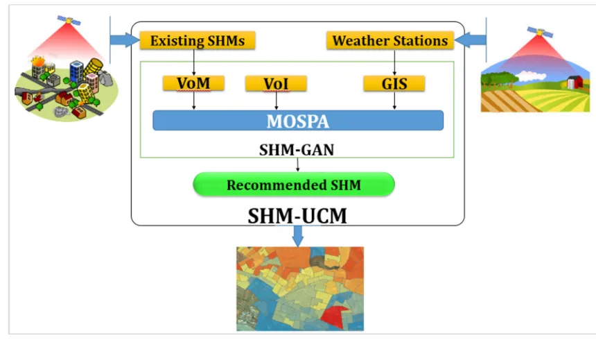
Figure 2. SHM-UCM
93
Figure 2 shows a complete overview of proposed SHM-UCM. It is evident that the data is taken
94
from Existing SHM systems, Weather Stations GIS and VoI, analyzed by proposed MOSPA algorithm
95
- resulting in SHM-GAN i.e. satellite-based system running MOSPA. This complete analysis of input
96
data and resulting in a geo plot for dynamically planning of SHM systems is ‘Structural Health
97
Monitoring Utility Computing Model’.
98
3. Structural Health Monitoring Systems
99
The Body Area Heterogeneous Network (BAHN) for the SHM system is designed for a structure
100
in which after hundreds of iterations in BIS frameworks, Value of Information is evaluated and
101
finalized by multi-disciplinary Subject Matter Experts inputs to ML algorithm. A SHM is a sequential
102
and systematic process in which the end product is a trustable abstract decision parameters dataset
103
based on the data collected from SHM system variables. Firstly, the SHM is developed and deployed
104
on structures-specific mandates that need to be monitored (e.g. residential, commercial, bridges,
105
tunnels). SHM system architecture is based on extracting upper and lower bounds of Finite Element
106
Analysis (FEA) data. By upper and lower bound we mean the maximum and minimum values at
107
which the structure is expected or meant to stay fully fit. A SHM system is a unique system that has
108
to serve the purpose for lifecycle evaluation of structure for a structure for the next 10 years.
109
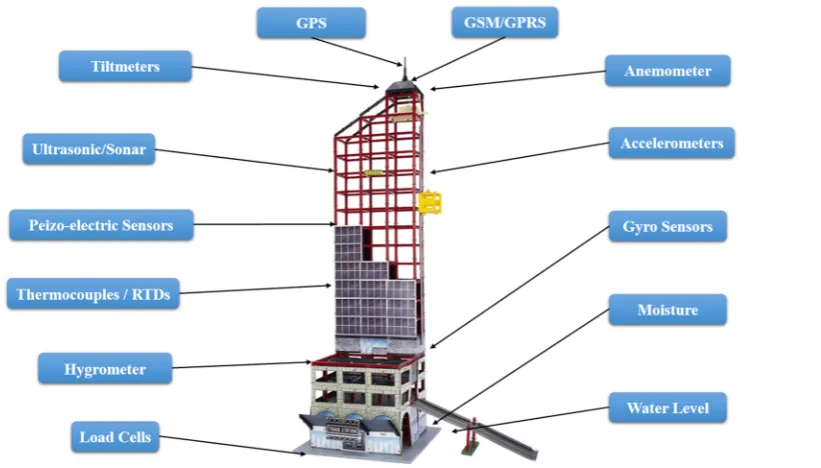
In Figure 3, a common SHM system has been shown based on Level of Detail 6 from BIS
110
documentation for a particular structure [refs]. This SHM system includes several sensors to measure
111
the structure health which includes weight (load cells), water level, moisture (hygrometer), balance
112
(gyro sensors), temperature (thermocouples or resistance temperature detectors), accelerometers
113
(vibration), pressure indoor and outdoor (piezo-electric sensors), collision or obstacle detection in
vicinity (ultrasonic sensors or sonar), tilt and inclination (tiltmeter) and wind speed (anemometer).
115
Secondly, the location and data communication is being achieved using GPS and GSM/GPRS,
116
respectively. The variables shown vary from structure to structure and is a complex set of the
117
formulation by a multi-disciplinary team. These variables can vary the SHM parameter estimation
118
and feature extraction; in other words, directly affect the technical assessment of VoI of the respective
119
structure. These SHM sensors have specific orientation and locations, which are calculated as per
120
geospatial constraints. These sensors vary based on VoI calculated for the building and expected
121
enormity of the disaster. This work is an effort toward the development of a smarter service oriented
122
UCM that will bring the multi-disciplinary procedures and practices under one umbrella called
SHM-123
UCM.
124
Figure 3. SHM by Lifecycle Management/Long Term Evolution
125
By 2018, the exponential rise in SHM nodes deployment has been registered across the world at
126
institutional and organizational level with different topologies, architectures, and frameworks on
127
various IoT platforms [17 – 18]. For in-situ long-haul seamless monitoring, a most successful and
128
frequent node architecture is used, which comprises a range of sensors, application specific scale
129
Signal Conditioners (SCs), and high-resolution Analog to Digital Converter (ADC) chips and
130
microcontrollers (e.g. Intel 8051, Microchip P18F458 and ATMega32).
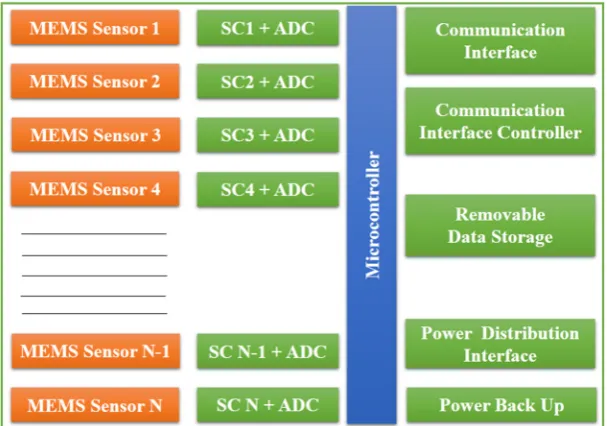
131
Figure 4 illustrates a typical SHM node used for heterogeneous Body Area Network (BAN)
132
implementations for existing SHM systems [19]. It has to go through a sequence of primitive data
133
processing methods to be compatible with SHM systems. This SHM Node has to be orchestrated like
134
a cloud framework ZeRo Client (ZRC), ThiN Client (TNC) and ThicK Client (TKC) nodes so that it
135
fits in the ecosystem of Industry 4.0 standard for SHM systems.
136
The SHM nodes proposed in this work are UCM coherent framework. The obligation of extreme
137
sensitivity, scalability and sampling frequencies is imposed to achieve the variable data processing
138
constraints for feature extraction techniques, Destructive Testing (NDT) methods, and
Non-139
Destructive Evaluation (NDE) procedures. It is repugnant to hire a new (different) team for detailed
140
SHM parameter assessment every time. A SHM-Application Specific Standard Part (SHM-ASSP) fills
141
the gap of providing the utility of high-resolution data for NDT and NDE assessment procedures.
142
In Figure 5, a SHM-ASSP ZRC Node is illustrated that includes MEMS Sensors along with
143
Programmable SC (PSC) to make it compatible with monitoring using specialized sensors and
144
Programmable ADC (PADC) that can adopt scaling and range recommendation for particular
145
observational criteria. The SHM-ASSP ZRC nodes proposed in this work need no external
instrumentation assistance for SHM operations. ‘STM32F10RBT6’ CPU interfaced with inclinometers
147
sensors are basic elements of nodes.
148
Figure 4. Conventional SHM Node Block Diagram
149
Figure 5. SHM-ASSP ZRC Node Block Diagram
150
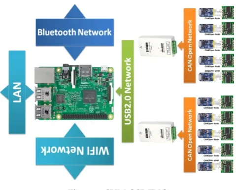
These nodes, which are developed in-house, are shown in Figure 6 and include:
151
• Seismic Sensors Node with 2 SHM Sensors
152
• Cylindrical Sensors Node full-fledged with 7 SHM Sensors
153
These nodes utilize CANopen industrial protocol paired with CAN-USB adapter to interface
154
with an Out-Surface Board (OSB), in case of underground deployment, that transfers sensors
155
readings wirelessly or wired to a gateway.
(a) SSN (b) CSN
Figure 6. SHM-ASSP ZRC Nodes
157
It is noteworthy to highlight that these nodes are enhanced with remotely programmable and
158
configurable parameters.
159
Figure 7. SHM-OSB TNC
160
Figure 7 shows an OSB that has a micro expert system with multiple resource-constrained
161
Machine Learning SHM Algorithm.
162
4. Multi-Objective SHM Prediction Machine Learning Algorithm
163
SHM is highly feasible for bigger structures, especially community buildings, where structure
164
value and human lives are critical. Multi-Objective SHM Prediction Machine Learning Algorithm
165
(MOSPA) takes into account the results for occupation count and SHM system parameters, then train
166
a ML algorithm to give a geo plot for the dynamic planning of SHM. It uses a multi-objective
167
Supervised ML Technique (SMLT) that streamlines the SHM Heterogeneous BAN architecture and
168
steps of installation recommended by SHM-UCM. For occupation count, Medium Access Control
169
(MAC) and International Mobile Equipment Identifier (IMEI) addresses along with biometric access
170
counter values are used. The final population count is obtained by removing the overlap between the
171
MAC, IMEI addresses and access counter using a condition-based methodology. Finally, SHM
172
parameters are used along with occupation data to obtain a geo plot for fitness view of SHM systems.
173
4.1 User Identification from MAC and IMEI Addresses
174
A two-tier mechanism for occupant counters has been employed as occupant space called 𝑂.
175
𝑂 is a sum of the number of MAC addresses registered in wireless routers (every PC or smart phone
176
has a Wi-Fi card or a LAN card that has MAC address) plus IMEI that every smart phone has as a de
facto de jure for Electronic Industry Association/Telecommunication Industry Association approved
178
the standard. These two variables overlap but gives a complete overview of all the electronic devices
179
in a particular location; mobile phones with SIM card and Devices connected to Wi-Fi.
180
𝑂 = 𝛴(𝑀𝐴𝐶) + 𝛴(𝐼𝑀𝐸𝐼) (1)
4.2 Attendance Count
181
For permanent inhabitants or occupants’ biometric access counter, 𝐼 is defined in terms of 𝑂
182
as:
183
𝑂 = 𝛴𝐼 (2)
Thus 𝑂 is summed up as
184
𝑂 = 𝑂 + 𝑂 (3)
The total occupancy probability distribution function is taken to obtain a random occupancy
185
vector at a specific location.
186
4.3 Final Population Count
187
In a given model [20, 21], hourly Probability Distribution Functions (PDFs) that allow the
188
calculation of the probability for a particular occupancy state occurring within a given hour is
189
presented. Let 𝐻 = (𝑂 · · · 𝑂 ) denotes all occupancies that occur per second during a period of
190
time and 𝑉 is a vector of occupancies for room 𝑥 where 𝑥 = 1,2, 3, … . 𝑦. Let 𝛼 denote the
191
average occupancy for the room 𝑟. We calculate a vector of means 𝛼 = (𝛼 , . . . , 𝛼 ) and covariance
192
matrix 𝑀 from 𝑂. Using 𝛼 and 𝑀, we define a Probability Density Function 𝑓:
193
𝑓 (𝑂; 𝛼, 𝑀) = 1 1
(2𝜋) |M| / exp −
(𝑂 − α) M (𝑂 − α)
2 (4)
Hourly Gaussian models with mean 𝛼 and covariance matrix 𝑀 , where 𝑓 can give a
194
probability of an occupancy occurring for a specific dataset 𝑂 for hour ℎ, is defined. Using this
195
function, random occupancy vectors can be drawn from the distribution.
196
The final population count is obtained by removing the overlaps between the MAC, IMEI
197
addresses and attendance count. A condition is applied that if the MAC, IMEI addresses are at a close
198
distance to a person counted for attendance, all should be counted as one person. Similarly, if
199
registered MAC s and IMEI addresses are at less than half a meter, it should be considered as single
200
person i.e. that person has a cell phone with IMEI address and a laptop with MAC address connected
201
to Wi-Fi but he or she has not put the attendance through biometric access count. Then after
202
calculating the final population count at a specific time step, a PDF can be obtained.
203
4.4 SHM Parameters
204
The BIM model is the second parameter value of information 𝑉𝑜𝐼 that has all the definitions
205
i.e. floors 𝐹 , beams 𝐵 , columns 𝐶 , stairs 𝑆 , rooms 𝑅 , halls 𝐻 , galleries 𝐺 ,
206
joints 𝐽 , trusses 𝑇 , payloads 𝑃 , areas 𝐴 and volumes 𝑉 . 𝑉𝑜𝐼 is a sum of
207
functions of joints, trusses, payloads and volumes [22].
208
𝑉𝑜𝐼 = 𝐹(𝐽 ) + 𝐹(𝑇 ) + 𝐹(𝑃 ) + 𝐹(𝑉 ) (5)
The applied physical fitness function [23] parameter, called 𝐹 , depends on the tilt 𝑇 ,
209
structural strain 𝛥𝐿/𝐿 , vibration 𝑉 , temperature 𝑇 , stress 𝑆 , wind effect 𝑊 , the
ground water level 𝐿 , humidity 𝐻 , moisture 𝑀 and composite material stability constant
211
𝑀 .212
𝐹 = 𝐹(𝑇 ) + 𝐹 𝛥𝐿 𝐿 + 𝐹(𝑉 ) + 𝐹(𝑇 ) + 𝐹(𝑆 ) + 𝐹(𝑊 ) + 𝐹(𝐿 )+ 𝐹(𝐻 ) + 𝐹(𝑀 ) + 𝐹(𝑀 ) (6)
Finally, the total population count along with the SHM fitness parameter can be used to train
213
the ML-based algorithm to propose real-time optimum location of SHM devices to mitigate risks
214
through better planning and early warnings. Nevertheless, this fosters covering wide area structures
215
and pinpoint any landmark changes that can affect the integrity of buildings. In the following section,
216
it can be clearly seen that the dynamic planning scheme of SHM systems, based on occupation count
217
and SHM real-time data.
218
5. Results and Discussion
219
The chosen case study is SHM system prediction for Qatar University (QU) from GAN based
220
SHM-UCM. The results of MOPSA are sequential in nature. First computation is runtime Variable
221
Occupancy Model (VoM) map based on the probability density function of occupancy 𝑂 given in
222
(4). The PDF in (4) forecasts the occupancy by adopting the historical random data of 𝑂, 𝛼 and 𝑀.
223
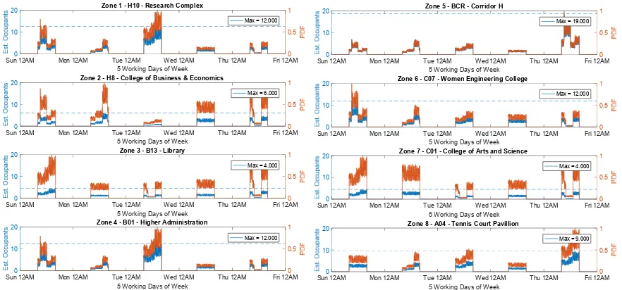
Figure 8. SHM Building Evaluation Graph
224
Figure 8 shows the simulation results obtained from the PDF in (4) by GAN selected zones based
225
on the estimated number of occupants per week (5 working days). The number of occupants must
226
not exceed the rated payload i.e. 50% of rated payload for a building in any zone. The results show
227
that maximum occupancy was observed in Zone 5: BCR Corridor H (19 persons), Zone 1: H10
228
Research Complex (12 persons) Zone 4: B01 (12 persons) and Zone 6: C07 (12 persons). Here, it is
229
worth mentioning that the results presented Figure 8 are simulated OSB based Figures, whereas
230
Figure 11 shows GAN output i.e. geo plot of QU, in which the cumulative result is taken from 8
231
different nodes running over the proposed algorithm in real-time. The predicted SHM has a private
232
cloud and a public cloud based on GAN.
233
Sun 12AM Mon 12AM Tue 12AM Wed 12AM Thu 12AM Fri 12AM
5 Working Days of Week
0 10 20 0 0.5 1
Zone 1 - H10 - Research Complex
Max = 12.000
Sun 12AM Mon 12AM Tue 12AM Wed 12AM Thu 12AM Fri 12AM
5 Working Days of Week
0 10 20 0 0.5 1
Zone 2 - H8 - College of Business & Economics
Max = 6.000
Sun 12AM Mon 12AM Tue 12AM Wed 12AM Thu 12AM Fri 12AM
5 Working Days of Week
0 10 20 0 0.5 1
Zone 3 - B13 - Library
Max = 4.000
Sun 12AM Mon 12AM Tue 12AM Wed 12AM Thu 12AM Fri 12AM
5 Working Days of Week
0 10 20 0 0.5 1
Zone 4 - B01 - Higher Administration
Max = 12.000
Sun 12AM Mon 12AM Tue 12AM Wed 12AM Thu 12AM Fri 12AM
5 Working Days of Week
0 10 20 0 0.5 1
Zone 5 - BCR - Corridor H
Max = 19.000
Sun 12AM Mon 12AM Tue 12AM Wed 12AM Thu 12AM Fri 12AM
5 Working Days of Week
0 10 20 0 0.5 1
Zone 6 - C07 - Women Engineering College
Max = 12.000
Sun 12AM Mon 12AM Tue 12AM Wed 12AM Thu 12AM Fri 12AM
5 Working Days of Week
0 10 20 0 0.5 1
Zone 7 - C01 - College of Arts and Science
Max = 4.000
Sun 12AM Mon 12AM Tue 12AM Wed 12AM Thu 12AM Fri 12AM
5 Working Days of Week
0 10 20 0 0.5 1
Zone 8 - A04 - Tennis Court Pavillion
Figure 9. SHM Building Evaluation Graph
234
Figure 9 shows cumulative fitness percentage of structures in Zone 1 to 8 obtained by the
235
estimated SHM system results (from (6)). Two colors of needles are visible in Figure 9, where the
236
golden ones show maximum overshoots or SHM with maximum utilization of structure, whereas the
237
black ones show that below 50% of sensors in SHM have almost constant values. The plots in Figure
238
9 are very realistic since indeed both H10 and H08 has a maximum flow of occupants that should
239
result in maximum vibration, the maximum change in pressure, humidity and temperature.
240
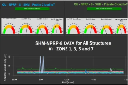
The developed private Cloud-based SHM-UCM GUI interface in Figure 10 shows instantaneous
241
results of SHM tiltmeter data and line plots of multiple zones (i.e. 1, 3, 5 & 7) being monitored and
242
analyzed by MOSPA. It illustrates how the data is uploaded over website over a public and private
243
cloud for different zones; in this case for zones 1, 3, 5 and 7 i.e. shown in Figure 9. The data of SHM
244
sensors (i.e. tiltmeters) can also be access over this cloud SHM-UCM platform either for a specific
245
zone or all together as in Figure 10. The tiltmeter data is in ‘meter per Second Square’ as it is obtained
246
from limited bandwidth of bi-axis accelerometer. This data is clear visualization for experts to make
247
a concise decision for optimum location of addition SHM sensors. In Figure 11, the main output
geo-248
plot is presented that comes as outcomes from automated decision-making map for helping
249
planning experts.
250
Figure 10. The dashboard of SHM-UCM predicted SHM
Figure 11. Geo Plot of Qatar University SHM Proposed Evaluation diagram
252
Figure 11 shows the resulting MOSPA geo plot that can be used for dynamic re-planning of
253
SHM. The dark yellow reading presents unfit conditions for structure health, whereas the dark green
254
indicates the fittest building (refer to Figure 9 for comparison). The unfit condition can be due to
255
several reasons such as critical historical building status or higher occupancy. The proposed
SHM-256
UCM model, working over the GAN satellite-based system, can be utilized as a tool for an in-depth
257
survey of geographical areas as well as disaster management.
258
6. Conclusion
259
A SHM utility computing model based on geographical area networks for real-time decision
260
making for a geospatial cluster has been proposed. Decision-making is made possible by a novel
261
Multi-Objective SHM Prediction Machine Learning Algorithm to process variables from
262
heterogeneous patches. The first variable was obtained from a Variable Occupancy Model and the
263
rest from a Building Information System. A case study was conducted on Qatar University buildings
264
to test the proposed algorithm. The results presented are an approximation of real-time analysis of
265
structures health and identified critical cases where more SHM nodes are required to efficiently
266
measure structural health for improved early warnings.
267
Author Contributions: Conceptualization, Hasan Tariq and Anas Tahir; Data curation, Hasan Tariq and Anas
268
Tahir; Formal analysis, Hasan Tariq and Anas Tahir; Funding acquisition, Farid Touati, Mohammed Abdulla E
269
Al-Hitmi, Damiano Crescini and Adel Ben Manouer; Investigation, Hasan Tariq and Anas Tahir; Methodology,
270
Hasan Tariq and Anas Tahir; Project administration, Farid Touati; Resources, Hasan Tariq, Anas Tahir and
271
Damiano Crescini; Software, Hasan Tariq and Anas Tahir; Supervision, Farid Touati; Validation, Hasan Tariq
272
and Anas Tahir; Visualization, Hasan Tariq and Anas Tahir; Writing – original draft, Hasan Tariq; Writing –
review & editing, Anas Tahir, Farid Touati, Mohammed Abdulla E Al-Hitmi, Damiano Crescini and Adel Ben
274
Manouer.
275
Funding: This publication was made possible by NPRP grant # 8-1781-2-725 from the Qatar National Research
276
Fund (a member of Qatar Foundation). The statements made herein are solely the responsibility of the authors.
277
Conflicts of Interest: The authors declare no conflict of interest. The funders had no role in the design of the
278
study; in the collection, analyses, or interpretation of data; in the writing of the manuscript, or in the decision to
279
publish the results.
280
References
281
1. Agdas, D., Rice, J., Martinez, J. and Lasa, I. (2016). Comparison of Visual Inspection and Structural-Health
282
Monitoring As Bridge Condition Assessment Methods. Journal of Performance of Constructed Facilities,
283
30(3).
284
2. Zaki, G., Plishker, W., Li, W., Lee, J., Quon, H., Wong, J., & Shekhar, R. (2016). The Utility of Cloud
285
Computing in Analyzing GPU-Accelerated Deformable Image Registration of CT and CBCT Images in
286
Head and Neck Cancer Radiation Therapy. IEEE Journal of Translational Engineering in Health and
287
Medicine, 1–11.
288
3. Yu, R., Ding, J., Maharjan, S., Gjessing, S., Zhang, Y., & Tsang, D. H. K. (2018). Decentralized and Optimal
289
Resource Cooperation in Geo-Distributed Mobile Cloud Computing. IEEE Transactions on Emerging
290
Topics in Computing, 72–84.
291
4. Olav Lysne, Sven-Arne Reinemo, Tor Skeie, Ashild Gronstad Solheim, Thomas Sodring, Lars Paul Huse
292
and Bjorn Dag Johnsen 2008, Interconnection Networks: Architectural Challenges for Utility Computing
293
Data Centers on IEEE Computer Society 2008.
294
5. Frey, H., & Gorgen, D. (2006). Geographical Cluster-Based Routing in Sensing-Covered Networks. IEEE
295
Transactions on Parallel and Distributed Systems, 17(9), 899–911.
296
6. Haiyan Xie, Tramel, J. M., & Wei Shi. (2011). Building Information Modeling and simulation for the
297
mechanical, electrical, and plumbing systems. 2011 IEEE International Conference on Computer Science
298
and Automation Engineering.
299
7. Li, W., Chen, H., & Xiang, B. (2012). The Study for GIS-based Distribution Network Monitoring and Control
300
Area Fault Location Methods. 2012 International Conference on Computer Science and Service System.
301
8. Haifeng Hu, Hengyuan Zhang, Wei Li. (2013). Visualizing Network Communication in Geographic
302
Environment. 2013 International Conference on Virtual Reality and Visualization.
303
9. Kurian, C. P., Milhoutra, S George, V. I. (2016). Sustainable building design based on building information
304
modeling (BIM). 2016 IEEE International Conference on Power System Technology (POWERCON).
305
10. Liaoning Jianzhu, (2016). Application Research of Building Information Model in the Construction Project
306
Life Cycle. 2016 International Conference on Smart Grid and Electrical Automation (ICSGEA).
307
11. Guodong Li, Junhua Zhang, Naiang Wang (2008). Construction and Implementation of Spatial Analysis
308
Model Based on Geographic Information System (GIS) - A Case Study of Simulation for Urban Thermal
309
Field. 2008 International Conference on Computational Intelligence for Modelling Control & Automation.
310
12. Giammarini, M., Isidori, D., Concettoni, E., Cristalli, C., Fioravanti, M., & Pieralisi, M. (2015). Design of
311
Wireless Sensor Network for Real-Time Structural Health Monitoring. 2015 IEEE 18th International
312
Symposium on Design and Diagnostics of Electronic Circuits & Systems.
313
13. Mahmud, M. A., Bates, K., Wood, T., Abdelgawad, A., & Yelamarthi, K. (2018). A complete Internet of
314
Things (IoT) platform for Structural Health Monitoring (SHM). 2018 IEEE 4th World Forum on the Internet
315
of Things (WF-IoT).
316
14. Monteiro, A., de Oliveira, M., de Oliveira, R., & da Silva, T. (2018). Embedded application of convolutional
317
neural networks on Raspberry Pi for SHM, Electronics Letters.
318
15. Sai Ji*, Ping Yang, Yajie Sun, Jian Shen, Jin Wang (2015). A New Mathematics Method for Structural Health
319
Monitoring’s Damage Detection Based on WSNs. 2015 First International Conference on Computational
320
Intelligence Theory, Systems and Applications (CCITSA).
321
16. D. Losanno, J.M. Londono, M. Spizzuoco (2013). A structural monitoring system for the management of
322
emergency due to natural events. 2013 IEEE Workshop on Environmental Energy and Structural
323
Monitoring Systems.
17. Varick L. Erickson, Merced Miguel A, Carreira Perpinan and Alberta E. Cerpa, Occupancy Modeling and
325
Prediction for Building Energy Management. (2014). Occupancy Modeling and Prediction for Building
326
Energy Management. ACM Transactions on Sensor Networks, 10(3), 1–28.
327
18. Dasyam, N. (2017). Structural Health Monitoring Market by Component (Hardware, Software, and
328
Services), Connectivity (Wired and Wireless), and End User (Civil, Aerospace, Defense, Energy, and
329
Others): Global Opportunity Analysis and Industry Forecast, 2017-2023. Engineering, Equipment, and
330
Machinery. [online] Allied Market Research, p.201. Available at:
331
https://www.alliedmarketresearch.com/structural-health-monitoring-market [Accessed 13 Oct. 2018].
332
19. Chang, F. (2013). Structural health monitoring 2013. Lancaster, Pa: DEStech Publ.
333
20. Tina Yu. (2010). Modeling Occupancy Behavior for Energy Efficiency and Occupants Comfort Management
334
in Intelligent Buildings. 2010 Ninth International Conference on Machine Learning and Applications.
335
21. Matteo Pozzi, Armen Der Kiureghiana. (2001) Assessing the Value of Information for long-term structural
336
health monitoring. Health Monitoring of Structural and Biological Systems.
337
22. Daniel Straub, Eleni Chatzi, Elizabeth Bismut, Wim Courage, Michael Döhler, Michael Havbro Faber,
338
Jochen Köhler, Geert Lombaert, Piotr Omenzetter, Matteo Pozzi (2017). Value of information: A roadmap
339
to quantifying the benefit of structural health monitoring. ICOSSAR - 12th International Conference on
340
Structural Safety.
341
23. Prasanna Tamilselvan, Yibin Wang, Pingfeng Wang (2012). Deep Belief Network based state classification
342
for structural health diagnosis.
343
24. Chong Du Mei Yuan Qiang You (2009). Study on the genetic algorithm used in damage identification.
344
25. Javier Rivera-Castillo, Moises Rivas-López, Juan I. Nieto-Hipolito, Oleg Sergiyenko, Wendy Flores-F.
345
(2014). Structural Health Monitoring based on Optical Scanning Systems and SVM.