Detection of Burr type XII Reliable Software
Using SPRT on Interval Domain Data
Dr. R. Satya Prasad1, B. Ramadevi2, Dr. G.Sridevi3
1Assoc.Prof, Department of CSE, Acharya Nagarjuna University, Guntur, India. 2ResearchScholor, Department of CSE, Acharya Nagarjuna University, Guntur, India.
3 Professor, Dept. of CSE, KL University, Vaddeswaram, Guntur, India.
Abstract– As the volumes of data/software is getting increased in the internet day by day, there is a need for the people to have the tools/mechanism to assess the software reliability as it takes more time to come to conclusion. In Classical Hypothesis first of all testing volumes of data is to be collected and later the conclusions are to be drawn which may take more time. In this paper a well known test procedure of statistical science called as Sequential Probability Ratio Test (SPRT) is adopted for Burr Type XII model in assessing the reliability of developed software. It requires considerably less number of observations when compared with the other existing testing procedures. Hence Sequential Analysis of Statistical Science could be adopted to decide upon the reliable / unreliable of the developed software very quickly. Besides the present paper proposes the performance of SPRT on Interval domain data using Burr type XII model and analyzed the results by applying on 6 data sets. The Maximum Likelihood Estimation is used for estimation of parameters.
Keywords: Burr Type XII model, Sequential Probability
Ratio Test, MLE, Software Reliability, NHPP.
I. INTRODUCTION
The SPRT was initially developed by Wald (1947) for quality control problems during World War II. It has many extensions and applications: such as in clinical trial and in quality control. The original development of the SPRT is used as a statistical device to decide which of two simple hypotheses is more correct. Wald’s SPRT is currently the only Bayesian Statistical procedure in SISA. What is required in Bayesian statistics is quite a detailed description of the expectations of the outcome under the model prior to executing the data collection. In Wald’s SPRT, if certain conditions are met during the data collection decisions are taken with regard to continuing the data collection and the interpretation of the gathered data. Wald's procedure is particularly relevant if the data is collected sequentially. Sequential Analysis is different from Classical Hypothesis Testing were the number of cases tested or collected is fixed at the beginning of the experiment. In Classical Hypothesis Testing the data collection is executed without analysis and Consideration of the data. After all data is collected the analysis is done and conclusions are drawn. However, in Sequential Analysis every case is analyzed directly after being collected, the data collected up to that moment is then compared with certain threshold values, incorporating the
new information obtained from the freshly collected case. This approach allows one to draw conclusions during the data collection, and a final conclusion can possibly be reached at a much earlier stage as is the case in Classical Hypothesis Testing. The advantages of Sequential Analysis are easy to see. As data collection can be terminated after fewer cases and decisions taken earlier, the savings in terms of human life and misery, and financial savings, might be considerable. In the analysis of software failure data we often deal with either Time between Failures or failure count in a given time interval. If it is further assumed that the average number of recorded failures in a given time interval is directly proportional to the length of the interval and the random number of failure occurrences in the interval is explained by a Poisson process then we know that the probability equation of the stochastic process representing the failure occurrences is given by a homogeneous Poisson process with the expression
! (1.1)
(Stieber 1997) observes that if classical testing strategies are used, the application of software reliability growth models may be difficult and reliability predictions can be misleading. However, he observes that statistical methods can be successfully applied to the failure data. He demonstrated his observation by applying the well-known sequential probability ratio test of (Wald 1947) for a software failure data to detect unreliable software components and compare the reliability of different software versions. In this paper we consider popular SRGM Burr Type XII model and adopt the principle of Stieber in detecting unreliable software components in order to accept or reject the developed software. The theory proposed by Stieber is presented in Section 2 for a ready reference. Extension of this theory to the SRGM – Burr Type XII is presented in Section 3.Maximum Likelihood parameter estimation method is presented in Section 4. Application of the decision rule to detect unreliable software components with respect to the proposed SRGM is given in Section 5.
II. SEQUENTIAL TEST FOR APOISSON PROCESS
Usefulness in development work on military and naval equipment it was classified as ‘Restricted’ by the Espionage Act (Wald 1947). A big advantage of sequential tests is that they require fewer observations (time) on the average than fixed sample size tests. SPRTs are widely used for statistical quality control in manufacturing processes. An SPRT for homogeneous Poisson processes is described below. Let {N(t),t 0} be a homogeneous Poisson process with rate ‘’. In our case, N(t) = number of failures up to time ‘t’ and ‘’ is the failure rate (failures per unit time ). Suppose that we put a system on test (for example a software system, where testing is done according to a usage profile and no faults are corrected) and that we want to estimate its failure rate ‘’. We cannot expect to estimate ‘’ precisely. But we want to reject the system with a high probability if our data suggest that the failure rate is larger than 1 and accept it with a high
probability, if it’s smaller than 0. As always with
statistical tests, there is some risk to get the wrong answers. So we have to specify two (small) numbers ‘α’ and ‘β’, where ‘α’ is the probability of falsely rejecting the system. That is rejecting the system even if λ ≤ 0. This is
the "producer’s" risk. β is the probability of falsely accepting the system .That is accepting the system even if λ ≥ 1. This is the “consumer’s” risk. With specified
choices of 0 and 1 such that 0 < 0 < 1, the probability
of finding N(t) failures in the time span (0,t ) with 1,0 as
the failure rates are respectively given by
!
(2.1)
! (2.2)
The ratio at any time ‘t’ is considered as a measure of deciding the truth towards , given a sequence of
time instants say ⋯ and the
corresponding realizations , … .Simplification of
gives
The decision rule of SPRT is to decide in favour of
, or to continue by observing the number of failures at a later time than 't' according as is greater than or equal to a constant say A, less than or equal to a constant say B or in between the constants A and B. That is, we decide the given software product as unreliable, reliable or continue (Satya Prasad 2007) the test process with one more observation in failure data, according as
(2.3) (2.4) (2.5)
The approximate values of the constants A and B are taken as ≅ , ≅
Where ‘’ and ‘’ are the risk probabilities as defined earlier. A simplified version of the above decision processes is to reject the system as unreliable if N(t) falls for the first time above the line
NU t a.t b2 (2.6)
To accept the system to be reliable if N(t) falls for the first time below the line
NL t a t b1
(2.7)
To continue the test with one more observation on , as the random graph of , is between the two linear boundaries given by Eq. (2.6) and (2.7) where
(2.8)
(2.9)
(2.10)
The parameters , , can be chosen in several
ways. One way suggested by Stieber (1997) is
log
1
If are chosen in this way, the slope of equals λ. The other two ways of choosing are from past projects (for a comparison of the projects) and from part of the data to compare the reliability of different functional areas(components).
III SEQUENTIAL TEST FOR SOFTWARE
RELIABILITY GROWTH MODELS
In Section 2, for the Poisson process we know that the expected value of called the average number of failures experienced in time 't' .This is also called the mean value function of the Poisson process. On the other hand if we consider a Poisson process with a general function (not necessarily linear) as its mean value function the probability equation of such a process is
!
,
0,1,2 …
Depending on the forms of we get various Poisson processes called NHPP, for our Burr type XII model. The mean value function is given as
( )
1 1
c b,
0
m t
a
t
t
We may write
!
!
Where , are values of the mean value function at specified sets of its parameters indicating reliable software and unreliable software respectively. The mean value function contains the parameters
′ ′,′ ′ ′ ′. Let , be values of the NHPP at two
specifications of b say , and two specifications of c say ,
.
It can be shown that for our model
at b1is greater than that at b0 and at c1 is greater than that at c0. Symbolically.
.
Then the SPRT procedure is as follows:Accept the system to be Reliable if
. .,
. .,
(3.1)Decide the system to be unreliable and Reject if
. .,
. .,
(3.2)
Continue the test procedure as long as
(3.3)
Substituting the appropriate expressions of the respective mean value function , we get the respective decision rules and are given in followings lines.
Acceptance Region:
0 1 0 1 0 0 1 1log 1 1
1 ( ) 1 log 1 b b c c b c b c
a t t
N t t a t
(3.4)
Rejection Region:
0 1 0 1 0 0 1 1 1log 1 1
( ) 1 log 1 b b c c b c b c
a t t
N t t a t (3.5) Continuation Region:
0 1 0 1 0 0 1 1lo g 1 1
1 1 lo g 1 b b c c b c b c
a t t
t a t
( )
N t
0 1 0 1 0 0 1 1 1lo g 1 1
1 lo g 1 b b c c b c b c
a t t
t a t (3.6)
It may be noted that in the proposed model the decision rules are exclusively based on the strength of the sequential procedure , and the values of the respective mean value functions namely, m0(t) , m1(t). If
the mean value function is linear in ′ ′ passing through origin, that is, the decision rules become decision lines as described by (Stieber 1997). In that sense equations (3.1), (3.2) , (3.3) can be regarded as generalizations to the decision procedure of Stieber(1997). The applications of these results for live software failure data are presented with analysis in Section 5.
IV MAXIMUM LIKELIHOOD ESTIMATION
In this section we develop expressions to estimate the parameters of the Burr type XII model based on interval domain data. Parameter estimation is of primary importance in software reliability prediction.
A set of failure data is usually collected in one of two common ways, time domain data and interval domain data. In this paper parameters are estimated from the interval domain data.
The mean value function of Burr type XII model is given by
( )
1 1
c bm t
a
t
(4.1)In order to have an assessment of the software reliability, a, b and c are to be known or they are to be estimated from software failure data. Expressions are now delivered for estimating ‘a’, ‘b’ and ‘c’ for the Burr type XII model. Assuming the given data are given for the cumulative number of detected errors ni in a given time interval (0, ti)
where i=1,2, ….. n and 0 < t1< t2< …tn, then the
1
1
1(
)log
( )
(
)
( )
k
i i i i k
i
LogL
n
n
m t
m t
m t
(4.2)
1
1
1
(
) log
1 1
1 1
1 1
k b b b
c c c
i i i i k
i
LogL
n
n
a
t
a
t
a
t
1
1
1
(
)
log 1
(1
)
(1
)
k b
c c b c b
i i i i k
i
LogL
n
n
Loga
t
t
a a
t
(4.3)
Taking the Partial derivative with respect to ‘a’ and equating to ‘0’.
(i.e.,
Log L
0
a
)1 1
(1
)
(
)
(1
)
1
c b k
k
i i c b
i k
t
a
n
n
t
(4.4)
The parameter ‘b’ is estimated by iterative Newton Raphson Method using
, Where ′ are expressed as follows.
0
1 11
1 1
1
(
1) .log(
1) (
1) log(
1)
log
1
log(
1)
(
1)
(
1)
( )
(n
)
1
1
(
1)
1
1
b b
i i i i
i i b b
k i i
i i
i
b
k k
t
t
t
t
t
t
t
t
Log L
g b
n
b
Log
t
t
(4.5)Again partial differentiating with respect to ‘b’ and equate to 0 , we get
2 '
2
( )
LogL
0
g b
b
1 1
1 2
2
1 '
2
1
1 2
1
1
2(
1) (
1) log(
1) log
1
(
)
(
1)
(
1)
( )
(
1) log(
1)
(
) log(1
)
(
1)
1
b b i
i i i
i
i i b b
k
i i
i
b k
k k
i i k b
i k
t
t
t
t
t
n
n
t
t
LogL
g b
b
t
t
n
n
t
t
(4.6)
The parameter ‘c’ is estimated by iterative Newton Raphson Method using
Where ′ are expressed as follows.
( )
LogL
0
g c
c
1 1 1
1 1 1
1 1 1 1
log
log
log
( )
(
)
log
log
(n
)
(1
)
(1
)
(t
)
(1
)
c c c c
k k
i i i i i i k
i i i c i c c c i i c
i i i i i i k
t
t
t
t
t
t
t
LogL
g c
n
n
t
t
n
c
t
t
t
t
(4.7)
′
0
1 1
1 2
2
1
' 2
1 1
2 2
1 2 2 1
1
1 2 2
1 1
.
log
log
(
)
( )
(
)
(
)(log ) .
(1
)
(log
) .
(log )
(1
)
(1
)
c c
i i i
i i
c c c
k k
i i i k
i i c c i i k c
i i i i k
i c i c
i i
t
t t
Log
t
t
t
t
t
t
Log L
g c
n
n
n
n
t
c
t
t
t
t
t
t
t
(4.8)
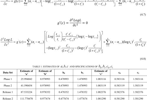
TABLE 1. ESTIMATES OF
a b c
, ,
AND SPECIFICATIONS OFb b c c
0, , ,
1 0 1Data Set Estimate of ‘a’
Estimate of
‘b’ b0 b1
Estimate of
‘c’ c0 c1
Phase 1 25.994042 0.978993 0.478993 1.478993 1.083116 0.583116 1.583116
Phase 2 41.590454 0.978993 0.478993 1.478993 1.083119 0.583119 1.583119
Release 1 87.533224 0.978352 0.478352 1.478352 1.082376 0.582376 1.582376
Release 2 111.778470 0.977674 0.477674 1.477674 1.081290 0.581290 1.581290
Release 3 59.376054 0.971698 0.471698 1.471698 1.051525 0.551525 1.551525
Release 4 42.831021 0.977671 0.477674 1.477674 1.081287 0.581287 1.581287
TABLE 2. SPRT ANALYSIS FOR 6 DATA SETS
Data Set T N(t)
R.H.S. of equation (3.4) Acceptance region
R.H.S. of equation (3.5) Rejection region
Decision
Phase 1 1 1 1.192028 1.856685 Accepted
Phase 2 1 3 1.792173 2.373032 Rejected
Release 1 1 16 3.338247 3.822450 Rejected
Release 2 1 13 4.089652 4.588755 Rejected
Release 3 1 6 2.430323 2.960544 Rejected
Release 4 1 1 1.839248 2.415563 Accepted
V SPRT ANALYSIS OF LIVE DATASETS
We see that the developed SPRT methodology is for a software failure data which is of the form [t, N(t)] where N(t) is the failure number of software system or its sub system in ‘t’ units of time. In this section we evaluate the decision rules based on the considered mean value function for Six different data sets of the above form, borrowed from (Pham 2005), (Wood 1996). Based on
the estimates of the parameter ‘b’ in each mean value function, we have chosen the specifications of
0
b
b
, b
1
b
c
0
c
and,c
1
c
equidistant on either side of b obtained through a data set to apply SPRT such thatb
0
b b
1 and0 1
Using the selected , , and subsequently the for each model we calculated the decision rules given by Equations (3.4), (3.5) sequentially at each ‘t’ of the data set taking the strength ( α, β ) as (0.05, 0.2).These are presented for the model in Table 2.
From Table 2 we see that a decision either to accept or reject the system is reached much in advance of the last time instant of the data (the testing time).
VI. CONCLUSION
In this paper, SPRT procedure is applied on the proposed model to detect reliable/unreliable software products. The Table 2 shows that Burr type XII SRGM as exemplified for 6 datasets indicates that the model is performing well in arriving at a decision. This model has given a decision of Acceptance for 2 datasets, Rejection for 4 datasets. The result of the present study indicates that the model is performing well in arriving at a decision. Therefore, we may conclude that the model Burr type XII is most appropriate model to decide upon reliability / unreliability of software.
REFERENCES
[1] GOEL, A.L and OKUMOTO, K. “A Time Dependent Error Detection Rate Model For Software Reliability And Other Performance Measures”, IEEE Transactions on Reliability, vol.R-28, pp.206-211, 1979.
[2] Pham. H., “System software reliability”, Springer. 2006. [3] Satya Prasad, R., ”Half logistic Software reliability growth model
“, 2007, Ph.D Thesis of ANU,India.
[4] Wald. A., “Sequential Analysis”, John Wiley and Son, Inc, New York. 1947.
[5] STIEBER, H.A. “Statistical Quality Control: How To Detect Unreliable Software Components”, Proceedings the 8th International Symposium on
Software Reliability Engineering, 8-12. 1997.
[6] WOOD, A. “Predicting Software Reliability”, IEEE Computer, 2253-2264. 1996.
[7] Xie, M., Goh. T.N., Ranjan.P., “Some effective control chart procedures for reliability monitoring” -Reliability engineering and System Safety 77 143 – 150¸ 2002.
[8] Michael. R. Lyu, “The hand book of software reliability engineering”, McGrawHill & IEEE Computer Society press. [9] Dr R.Satya Prasad, G.Krishna Mohan and Prof R R L Kantham.
Article: Time Domain based Software Process Control using Weibull Mean Value Function. International Journal of Computer Applications 18(3):18-21, March 2011.
[10] Musa, J.D., Iannino, A., Okumoto, k., 1987. “Software Reliability: Measurement Prediction Application”. McGraw – Hill, New York.