Estimating fractional snow cover in open terrain from Sentinel-2 using the normalized difference snow index

Article

Estimating fractional snow cover in open terrain from

Sentinel-2 using the normalized difference snow

index

Simon Gascoin 1,_{*, Zacharie Barrou Dumont} 1_{, César Deschamps-Berger} 1,2,_{, Florence Marti} 3_, Germain Salgues 3_{, Juan Ignacio López-Moreno} 4_{, Jesús Revuelto} 4_{, Timothée Michon} 5_{, Paul} Schattan 6 _{and Olivier Hagolle} 1

1 _{CESBIO, Université de Toulouse, CNES/CNRS/INRA/IRD/UPS, Toulouse, France}

2 _{Université Grenoble Alpes, Université de Toulouse, Météo-France, CNRS, CNRM, Centre d'Etudes de la} Neige, Grenoble, France

3 _{Magellium, Toulouse, France}

4 _{Pyrenean Institute of Ecology, CSIC, Zaragoza, Spain} 5 _{Tenevia, Grenoble, France}

6 _{University of Innsbruck, Institute of Geography, alpS Research, Austria}

* Correspondence: [email protected]

Abstract: Sentinel-2 provides the opportunity to map the snow cover at unprecedented spatial and temporal resolution at global scale. Here we calibrate and evaluate a simple empirical function to estimate the fractional snow cover (FSC) in open terrain using the normalized difference snow index (NDSI) from 20 m resolution Sentinel-2 images. The NDSI is computed from flat surface reflectances after masking cloud and snow-free areas. The NDSI-FSC function is calibrated using Pléiades very high resolution images and evaluated using independent datasets including SPOT 6/7 satellite images, time lapse camera photographs, terrestrial lidar scans and crowd-sourced in situ measurements. The calibration results show that the FSC can be represented with a sigmoid-shaped function 0.5×tanh(a×NDSI+b)+0.5 where a = 2.65 and b = -1.42 yielding a root mean square error of 25%. Similar RMSE are obtained with different evaluation datasets with a high topographic variability. With this function, we estimate that the confidence interval on the FSC retrievals is 38% at the 95% confidence level.

Keywords: snow; snow cover area; fractional snow cover; Sentinel-2

1. Introduction

The Global Observing System for Climate listed the snow cover as one of the 50 essential climate variables to be monitored by satellite remote sensing to support the work of the United Nations Framework Convention on Climate Change and the Intergovernmental Panel on Climate Change [1]. Among the many variables that can be used to characterize the snow cover, the snow cover area is probably the most straightforward to retrieve from space [2,3]. Yet, it is one of the most important as it serves as an input to address research questions in various fields including climate science, hydrology and ecology. The snow cover area is also important to support other societal benefit areas like water resource management, transportation and winter recreation. A user requirements survey by the Cryoland consortium showed that snow cover area products were ranked as the most important among a list of operationally available remotely sensed snow products by the respondents [4]. The respondents also emphasized the need for (i) short latency times in the product availability

(shorter than 12 h) (ii) large spatial scale to cover entire mountain ranges like the Alps or even the

whole of Europe (iii) high spatial resolution down to 50 m resolution especially for road conditions

and avalanches monitoring [4].

While the operational monitoring of the snow cover area at global scale has been achieved since

the 2000’s using wide swath optical sensors like MODIS [2], the low spatial resolution of the products

(typically 500 m) usually does not enable to address operational applications such as the above. Many scientific applications would also benefit from higher resolution information on the snow cover area. For instance, high resolution maps of the snow cover area were critical to explain the spatial diversity of plant communities in an alpine grassland [5,6]. High-resolution snow cover area is also useful in hydrology to reduce biases in the spatial distribution of the snow water equivalent through data assimilation [7], in particular in semi-arid mountain regions [8,9].

The Sentinel-2 mission, which images the land surface at high resolution with a 5-day revisit time and a global coverage offers the unique opportunity to bridge this gap [10,11]. As part of the Copernicus program, the Sentinel-2 mission is planned to run continuously for at least two decades. Based on the above, the Theia land data center in France has supported the deployment of an operational service to generate and distribute at no cost snow cover maps derived from Sentinel-2 (20 m resolution) and Landsat-8 (30 m resolution) [12]. However, this product only provides a binary description of the snow cover area in the pixel (snow or no-snow, hereafter referred to as SCA). The SCA mapping may be insufficient to characterize the snow distribution in areas where partially snow-covered (mixed) pixels are prevalent [13–15]. Using 0.5 m resolution satellite imagery, Selkowitz et al. [14] quantified the frequency of occurrence of mixed pixels over five dates at two study areas in the western U.S. Their results show that in the study area with maritime climate, the fraction of mixed pixels at the typical Sentinel-2 resolution (20 m) is below 40%, whereas it can reach 80% in a more continental mountain area. Binarizing pixels in snow or no-snow in areas where mixed pixels are prevalent can introduce an error in the spatial integration of snow cover area, e.g. when the snow cover area is computed over a watershed[14].

The Fractional Snow Cover (FSC), i.e. the snow-covered fraction of the pixel area, naturally provides a finer information than the binary SCA. However, it does not necessarily mean that it provides a more accurate information. The estimation of the FSC from multi-spectral images is challenging due to the confounding effects of the snow, rocks and vegetation surfaces on the spectral signature of pixel reflectance [16]. Therefore, it is important to evaluate the accuracy of the retrieved FSC by comparing with independent observations to make sure that the gain in precision is worth the additional cost of computing and storage.

The spectral signature of a pixel can be modelled as a linear combination of the spectra of the pure surface materials, or endmembers thought to be present in it [17–19]. However, the spectral unmixing approach is challenging to use in operational context: (i) it amounts to an ill-posed problem which requires a computationally intensive inversion step to estimate the relative abundance of each endmember; (ii) it requires prior knowledge of a collection of endmembers that covers the range of natural surfaces to be observed (geology, vegetation). Such requirements are hardly compatible with those from the users (timeliness, high resolution, large spatial scale).

Another option is to use the Normalized Difference Snow Index (NDSI) [20] as a mean to retrieve the FSC through empirical regression. Previous studies involving lower-resolution sensors like MODIS and SPOT VEGETATION have shown positive results using a linear function or a generalised logistic function to estimate the FSC from the NDSI [21,22]. A linear function was used by the NASA in operational context to generate the FSC from collection 5 MODIS surface reflectance products (MOD10A1.005 and MYD10A1.005) [23]. The current operational MODIS snow product does not provide the FSC anymore but still provides the NDSI as a mean to retrieve the FSC using custom equations [24]. A recent comparison of spectral unmixing and NDSI regression methods to estimate FSC with Sentinel-2 data showed that even an uncalibrated linear regression can yield nearly similar performance to the spectral unmixing [15]. This result was obtained despite the fact that endmembers for the spectral unmixing algorithm were chosen to match the characteristics of the study area (a high Arctic site). Apart from this study, to our best knowledge, there is no previous evaluation of the NDSI-FSC relationship from Sentinel-2 data.

this relationship, we endeavour to use a large amount of data covering a range of environments and seasons. We wish to evaluate if the error is stable across different sites and seasons.

We build this work upon our previous efforts that led to the implementation of the Theia snow collection. The Theia snow products are currently generated by the LIS software version 1.5 (https://gitlab.orfeo-toolbox.org/remote_modules/let-it-snow/). The LIS algorithm already relies on the NDSI to determine the snow-covered pixels (hereinafter referred to as the LIS-SCA algorithm). The NDSI is computed from level-2A products, i.e. slope corrected surface reflectance images including a cloud and cloud shadow mask. The current configuration uses level-2A products generated by MAJA software. MAJA is an operational level-2A processor, which implements a multitemporal algorithm to estimate the aerosol optical thickness and make an accurate classification of cloud pixels [25,26]. The MAJA-LIS workflow was evaluated using in situ and remote sensing data [12]. The results showed that the snow cover area was accurately detected [12], and that the snow detection was more accurate than the Sen2Cor outputs [27].

We proceed as follows. First, we calibrate the function f whichassociates an FSC value to an NDSI value:

FSC = f(NDSI), (1)

where f is a continuous, monotonically increasing function. The calibration is done using a set of very high-resolution satellite images, which provide accurate reference snow maps. Then, we evaluate this function in independent sites where we have reference data from various sources. Section 2 presents the data and methods used to perform such calibration and evaluation. In Section 3 we describe the results and discuss them in Section 4.

2. Data and Methods

2.1. Calibration

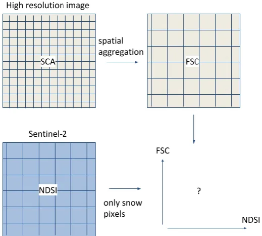
We used five clear-sky Pléiades tri-stereoscopic images to calibrate the NDSI-FSC function. This was done by generating accurate maps of the snow cover area at 2 m resolution from the Pléiades data, which were then resampled to obtain reference maps of the FSC at the same resolution of the NDSI (20 m) (Fig. 1).

Figure 1. Schematic of the method used to determine the NDSI-FSC relationship. In this study the spatial aggregation is done using the average of all contributing pixels unless there is at least

All selected Pléiades images were acquired over the same pilot site of 140 km2 _{in the French}

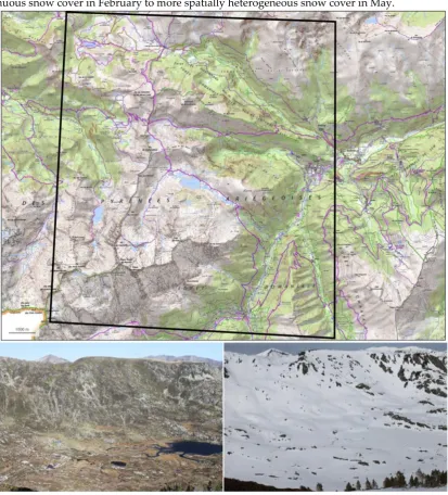
Pyrenees after 2016 (Bassiès catchment, [28]). The elevation of the study area ranges between 730 and 2676 m a.s.l., with a contrasting topography and geology (Fig. 2). In low-elevation regions, the vegetation is mainly formed by coniferous and deciduous trees; at middle elevations, between 1400 and 2000 m a.s.l., the surface is covered by grassland, rangeland and subalpine meadow; and above 2000 m a.s.l., vegetation is scarce and the surface is made of bare crystalline rock (granite and granodiorite) or fluvio-glacial deposits, except in the north of the domain where metamorphosed limestones are found [29]. The images were acquired between February and May between 2016 and 2019 (Table 1), providing information on different snow cover conditions, ranging from rather continuous snow cover in February to more spatially heterogeneous snow cover in May.

Figure 2. Top: topographic map of the Bassies area (42°45’N, 1°25’E in the Pyrenees, France). The

black polygon indicates the outline of the Pléaides acquisition (source: IGN/SCAN25, www.geoportail.gouv.fr). Bottom: photographs taken from Col de la Serrette near the geographic center of the study area (26 Oct 2014, 11 Mar 2015).

the UTM reference system. All Pléaides DEMs were aligned to the same reference DEM, which is known to have a horizontal offset of 3.0 m from the north and -0.8 m from the east (standard deviation 0.4 m) from control points obtained from an aerial orthophoto (see Table 2 in [28]). Hence this horizontal translation was applied to all Pléaides images before comparing them with Sentinel-2 to avoid introducing errors due to inaccurate geolocation of Pléiades data.

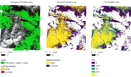
The resulting Pléaides multispectral orthoimages were used to generate the SCA maps of the five acquisitions with a pixel-based supervised classification. For each date, the few cloud pixels were manually delineated to restrict classification to cloud-free areas. The same procedure was applied to water bodies. Then we manually delineated about 15 homogeneous polygons of snow and no-snow surfaces (ground and vegetation) based on a colour composite of the multispectral image which enhances the contrasts between rocks, water, vegetation and snow (NIR/red/green bands). These polygons were used to extract samples to train a random forest classifier with the Orfeo Toolbox [31] as done above with the SPOT data (Sect. 2.1.2). The resulting 2 m SCA maps (Fig. 3, middle panel) were then downsampled to obtain 20 m FSC maps by computing the weighted average of all contributing pixels. If there was at least one no-data pixel among the contributing pixels then the FSC value was set to no data (Fig. 3, right panel).

Figure 3. Illustration of the processing workflow from the Pléiades multispectral image to the reference FSC map.

To evaluate the performance of the SCA classification in Pléiades images, we constructed an independent validation dataset. First a mask of the non-forest area was extracted from the 2015 Copernicus Tree Cover Density (TCD) product at 20 m resolution (i.e. areas where TCD = 0). This mask was eroded using a disk of radius 3 pixels to remove unidentified mixed pixels near the edges of the forest area. Then, 30 random points were created within this non-forest mask. A different

person from the one who created the samples to train the classifier assigned the value ‘snow’ or ‘no

-snow’ to each point for each date based on the visual inspection of the color composite of the multispectral image. This formed a set of 150 validation points that were used to compute performance metrics derived from the confusion matrix (accuracy, false-positive rate, false-negative

rate, F1 score, kappa coefficient; see section 2.1.3).

snow-covered pixels were determined with the LIS-SCA algorithm. The NDSI of these snow pixels was computed from the L2A product (flat surface reflectance). All images were mostly cloud-free (< 5% cloud cover) over the study area, but the few visible cloud pixels were masked. All pixels with a positive TCD were excluded.

Pléiades 2016-04-11 2017-03-15 2018-02-15 2018-05-11 2019-03-26

Sentinel-2 2016-04-11 2017-03-14 2018-02-15 2018-05-11 2019-03-27 Table 1. Dates of the Pléiades and Sentinel-2 dataset pairs to calibrate and validate the NDSI-FSC relationship.

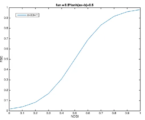
The Sentinel-2-derived NDSI and Pléiades-derived FSC datasets were paired on a pixel basis forming a list of approximately 6.4e5 pairs which was randomly split in two subsets to perform the calibration and validation: 60% as a training dataset (for calibration) and 40% as a testing reference dataset (for validation). A nonlinear function with a sigmoid shape was chosen to represent the NDSI-FSC relationship because preliminary tests using an affine function were not satisfactory (not shown here). The following function was used:

FSC = ½ (tanh(a NDSI + b) +1) (2)

Figure 4. Shape of the function used to estimate the FSC from NDSI.

Figure 4 illustrates the shape of this function with a = 3 and b = -1. Parameters a and b were optimized using the root-mean-square error (RMSE) between the predicted FSC and the training FSC as the objective function to minimize. This optimization was done with the Nelder-Mead simplex algorithm as implemented in the SciPy library [32]. Once the NDSI-FSC relationship was calibrated, it was validated against the Pléiades testing dataset using standard metrics (section 2.2.4).

2.2. Evaluation

2.2.1. Evaluation with remote sensing data

● SPOT: five SPOT-6 and SPOT-7 maps of the snow cover area at 6 m resolution obtained by supervised classification [12]. Each SPOT scene covers a region of about 2900 km2_.

● Izas: a series of 758 SCA maps at 1 m resolution in the Izas catchment located in the Spanish Pyrenees. These snow maps were derived from a series of daily photographs taken between 2015 and 2019 by a terrestrial time-lapse camera (CC5MPX Campbell Sci.). The processing of the photographs to orthorectified SCA maps is described by Revuelto et al. [33]. The images cover an area of about 0.3 km2_.

● Weisssee: a series of nine SCA maps at 0.5 m resolution around the Weisssee Snow Research Site (Austria). These snow maps were derived from terrestrial laser scans presented by Fey et al. [34]. The discrimination of snow-covered and snow-free areas was based on surface reflectance and snow depth. The scans cover a region of about 0.9 km2 _{with differing slopes}

and vegetation cover.

● CamSnow: a series of 351 FSC maps at 25 m resolution of the Aiguilles Rouges massif near Chamonix, France. These maps were derived from a series of daily photographs taken from 2016 to 2019 with a time-lapse camera installed in the Aiguille du Midi. The processing was done by TENEVIA, a start-up company specialized in the hydrometeorological monitoring of high mountain catchments. The images cover an area of about 50 km2_.

● DISCHMEX: a series of five SCA maps at 0.2 m resolution in the Dischma valley near Davos, Switzerland [35]. The snow cover area was retrieved from aerial ortho-images over a region of about 0.1 km2_.

All the SCA data were resampled from their original projection to the projection system of the corresponding Sentinel-2 tile (WGS84 UTM 30N, 31N or 32N) at 20 m resolution by taking the average of the contributing pixels. As done in section 2.2.1, if at least one pixel in the contributing pixels is a no-data pixel, the corresponding FSC pixel is also a no-data pixel to avoid introducing sampling biases.

Once an FSC product was matched with a Sentinel-2 acquisition (see section 2.2.5), we selected the Sentinel-2 pixels marked as snow-covered by LIS SCA algorithm and computed their NDSI (as done in section 2.2.1). The NDSI was then converted to FSC using the calibrated function obtained from section. 2.2.1. As a result, for each dataset, we obtained a list of reference FSC values that are collocated in space and time with a list of Sentinel-2 FSC values. This allowed a comparison at the Sentinel-2 pixel level, using the metrics defined in section 2.2.4.

We handled the case where the FSC reference map can overlap two Sentinel-2 tiles (only SPOT). In this case, the SPOT product was cropped using the Sentinel-2 tiles extent and each portion was processed independently. In this process we made sure that the overlapping region between two Sentinel-2 tiles was not counted twice.

Figure 5. Map of the datasets used for FSC evaluation. More information on the SPOT images is given in [12].

2.2.2. Evaluation using crowd-sourced data

Figure 6. Presentation of the ODK Collect initiative used to collect crowded-sourced snow fraction data.

The ODK FSC was directly compared to the FSC of the nearest pixel in the matching Sentinel-2 product, using the metrics defined in section 2.2.4 below. Section 2.2.5 explains how this matching product is identified. Measurements made in forest areas were identified using the TCD product (i.e. where TCD > 0, section 2.2.1) and removed from this analysis.

2.2.3. Sensitivity to the temporal collocation method

Because Sentinel-2 acquisitions are not necessarily synchronized with other products, a reference FSC may have to be matched with a Sentinel-2 FSC product from a different date. In addition, the closest Sentinel-2 FSC product in time may not be the best choice in case of cloudy conditions so that it might be useful to find the next closest product to increase the amount of evaluation data. However, the snow cover extent can change rapidly so it is necessary to bound the time search window that is used to match a reference product with a Sentinel-2 product. This is particularly important for dates before July 2017 (Sentinel-2B operation start date) when the revisit time of Sentinel-2 was only 10 days.

We also tested the sensitivity of the selection criteria to match a reference product with a Sentinel-2 product. Indeed, within a given time window around the date of the reference products, one could find several Sentinel-2 products. We tested the following two options:

● closest date: the Sentinel-2 product that is the closest in time to the FSC product is selected.

● cleanest date: the Sentinel-2 product with the least cloud and no-data pixels is selected. Both options were tested for different time windows from 0 to 4 days (for 0 days both methods are identical).

This issue is specific to FSC evaluation, where we must handle heterogeneous datasets with uneven temporal frequency such as ODK or CamSnow. This was not a problem in previous sections where Sentinel-2 FSC was compared either with daily snow depth measurements or a few Pléiades and SPOT images for which manual selection was possible.

2.2.4. Evaluation metrics

For each type of high-resolution remote sensing, from all pairs of Sentinel-2 and reference data, we derive the following metrics: RMSE (root mean square error between the predicted and the observed FSC), mean error (mean of the differences between the predicted and the observed FSC), STD (standard deviation of the differences between the predicted and the observed FSC) and

correlation (Pearson’s correlation coefficient between the predicted and the observed FSC).

3. Results

3.1. Calibration

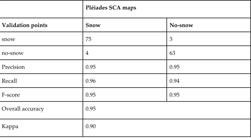
Table 2 shows the confusion matrix between the Pléaides SCA maps at 2 m resolution and the 150 validation points. Among the 150 points, 5 were not classified due to the presence of clouds or because no decision was made by the analyst. The derived kappa and overall accuracy above 0.9 suggest that the Pléiades images have been correctly classified. This was expected from the visual evaluation of the Pléaides SCA maps which showed that the supervised random forest classifier allows an efficient classification of the snow areas given the high contrast with snow-free areas in the visible-NIR region of the spectra.

Pléiades SCA maps

Validation points Snow No-snow

snow 75 3

no-snow 4 63

Precision 0.95 0.95

Recall 0.96 0.94

F-score 0.95 0.95

Overall accuracy 0.95

Kappa 0.90

The calibration of the NDSI-FSC function with the Pléiades data returned the values a = 2.65 and

b = -1.42 with an RMSE of 25% (Fig. 7). In validation mode, the same RMSE was obtained, suggesting that the estimation of the error is robust (Table 3).

Figure 7. Results of the calibration and validation of the function. Upper left panel: 2D histogram plot of the FSC and NDSI pairs in the training dataset and optimized function. Upper right panel: 2D histogram plot of the predicted FSC vs. the testing FSC dataset. Red line: calibrated NDSI-FSC function. Blue line: Linear regression between the predicted and the testing FSC sets. Green line: 1:1 line. The colour bar indicates the number of samples by bin. Bottom: histogram of the residuals for the validation (predicted FSC minus FSC test).

Metric Value

Sample size 254664

RMSE 25%

Mean error -0.9%

Standard deviation 24%

Correlation 0.60

Table 3. Validation of the predicted FSC against the testing dataset (Pléiades data).

3.2. Sensitivity to the temporal collocation method

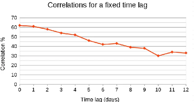
Figure 8 Evolution of the correlation coefficient between Sentinel-2 NDSI and Izas FSC as a function of the time lag.

Figure 9 illustrates the tradeoff between the ‘cleanest’ and ‘closest’ approaches in selecting the

matching Sentinel-2 product. The number of pixels is higher with the cleanest method since this method selects the least cloudy image in a given time window, but the correlation coefficient is lower than the correlation coefficient of the closest method beyond 3 days, for the same reason as given in Fig. 10. However, this analysis suggests that the difference between both methods is minimal. Given

that the ‘closest’ method is numerically more efficient we kept this method with a time window of 4

days to perform the next analyses.

Figure 9. Evolution of the correlation coefficient between Sentinel-2 NDSI and Izas FSC and

evolution of the number of pixels as a function of the time lag (plus or minus) for the ‘cleanest’ and ‘closest’ approaches.

3.3. Evaluation with remote sensing data

The results are presented for each remote sensing data used:

● Izas: all available dates were merged as a single dataset. Despite the small size of the Izas study area, a large number of FSC values could be used thanks to the long duration of the time series and its near daily frequency (N=4.5e4). The results are in line with the previous evaluations with an RMSE of 21% and a mean error of -11% (Table 6). The correlation coefficient of 0.61 indicates that the NDSI-FSC function provides a correct representation of the FSC in the Izas catchment.

● Weisssee: all available dates were also merged as a single dataset (Table 6). The correlation (0.42) is lower than the one obtained with Izas data but the RMSE is improved (18%). This is because this dataset is skewed towards high FSC values, which tend to penalize the correlation with respect to the RMSE or the standard deviation (0.13).

● CamSnow: the comparison was done using the time series of average FSC over the study area (181 dates). Due the spatial aggregation which tend to decrease the random error, the performance of the FSC algorithm is acceptable with a correlation coefficient of 0.43, a RMSE of 20% and a mean error close to zero (-1.8%) (Table 6). However, it should be noted that the same type of evaluation using the mean spatial FSC was done with Izas data and the correlation coefficient is higher 0.94 (437 dates, Table 6). This suggests that the performance of CamSnow data may be affected by their inaccurate geometry and may not reflect the actual accuracy of the Sentinel-2 FSC (section 2.2.2).

● DISCHMEX: We found that there were too few valid data in the DISCHMEX images to make an evaluation. This was due to the presence of many missing values in the original data and the fact that our resampling method considers that a resampled pixel becomes a no-data pixel if there is at least one no-data pixel in the contributing pixels.

Sentinel-2 tiles

SPOT 2016-08-08

SPOT 2017-03-11

SPOT 2016-12-03

SPOT 2016-12-17

SPOT 2016-10-12

T32TLR 2016-08-10 2017-03-11 2016-12-01 2016-12-18 2016-10-12 T32TLQ 2016-08-10 2017-03-11 2016-12-01 2016-12-18

T31TGK 2016-08-06 2017-03-11 2016-12-01 2016-12-14

T31TGL 2016-08-06 2017-03-11 2016-12-01 2016-12-14 2016-10-12

T31TGM 2016-10-12

T32TLS 2016-10-12

Table 4. Pairs of SPOT and Sentinel-2 products used to perform the evaluation shown in Table 5.

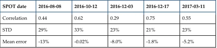
SPOT date 2016-08-08 2016-10-12 2016-12-03 2016-12-17 2017-03-11

Correlation 0.44 0.62 0.29 0.75 0.55

STD 29% 33% 23% 21% 23%

RMSE 31% 33% 25% 21% 24% Table 5. Evaluation of the Sentinel-2 FSC against the SPOT FSC.

Site Izas Weisssee CamSnow Izas

Level Pixel Pixel Area Area

Sample size 44890 2492 181 437

RMSE 21% 18% 20% 18%

Mean error -12% -12% 3.5% -10%

STD 18% 13% 21% 16%

Correlation 0.61 0.42 0.43 0.93

Table 6. Evaluation of the Sentinel-2 FSC with Izas and Weisssee FSC (20 m pixel-based comparison), and CamSnow and Izas mean FSC (in percentage of the imaged area).

3.4. Evaluation with crowd-sourced in situ data

Table 7 summarizes the data that were contributed by the participants. After removing the data with a geolocation accuracy higher than 5 m, and data for which the LIS-SCA algorithm does not detect snow, we retained 337 FSC values. Among these 337 values, 141 were collected in areas with TCD > 0 (Tab. 10).

TILE

AVAILABLE ODK

POINTS ACCURACY≤5m

ACCURACY≤5m

AND LIS-SCA PIXEL=SNOW

TCD>0 TCD>0 TCD>0

T31TDH 344 222 137

T30TYN 12 9 4

T31TGL 5 2 0

T31TCH 4 3 0

T32TLP 0 0 0

T31TGK 1 1 0

T32TLQ 0 0 0

T31TFL 0 0 0

T31TFK 0 0 0

TOTAL 366 237 141

Table 7. Summary of the ODK Collect data obtained on March 15, 2020. In bold is the total number of collected ODK FSC eventually used for the Sentinel-2 FSC evaluation.

The comparison shows that there is a good agreement between the Sentinel-2 FSC and the ODK measurements with an RMSE that is again close to 25% (Table 8, Fig. 10).

Metric FSC

Sample size 337

RMSE 23%

Mean error -7.2%

Standard deviation 21%

Correlation 0.67

Table 8. Evaluation of the Sentinel-2 FSC against the ODK data.

Figure 10. Results of the evaluation of the FSC using ODK data. Blue line: Linear regression between the predicted and the testing FSC sets. Green line: 1:1 line. The colour bar indicates the number of samples by bin.

4. Discussion

In both calibration or in evaluation sections, we obtained larger RMSE than previous studies using MODIS data to compute the FSC at coarser resolution for operational production. Salomonson and Appel [21] reported RMSE ranging between 4% and 10% for test sites over Alaska, Labrador, and Siberia by comparison with Landsat SCA products. These results were obtained with a linear function which formed the basis of the MOD10A1.005 product algorithm. Using Landsat-8 SCF products, Rittger et al. [13] obtained an average RMSE of 10% with MODSCAG products. However, Rittger et al. [13] reported higher RMSE of 23% for MOD101A1.005 and Masson et al. [19] found larger RMSE for both MODSCAG and MOD10A1.005 ranging between 25%-33%.

resolution, and spatial aggregation from 20 m to 100 m is expected to reduce the error variance. In addition the model was only tested over a small region of 1.77 km2 _{with a low topographic variability}

of (elevation range of 50 m). The same authors found that the error variance of FSC retrieved by spectral unmixing was larger for intermediate FSC and lower for high and low FSC residuals. Here we could not identify a similar behaviour, although another form of heteroscedasticity is manifest in the Pléiades-derived FSC residuals from Section 3.1 (Figure 11). This dataset suggests that the error has a larger variability for low FSC retrievals.

Figure 11. Variance of the residuals of the FSC retrievals from the Pléiades validation dataset (Sect. 3.1)

Neglecting heteroscedasticity and assuming that the FSC residuals follow a gaussian distribution of

zero mean and standard deviation σ, we can estimate the probability that a retrieval of SCF=0 is significantly different than SCF=1 at the pixel level. With the Normal inverse cumulative distribution

function, we can estimate that σ should not exceed 61% otherwise a retrieval of SCF=0 would not be

significantly different than SCF=1 at the 5% confidence level. Here, we obtained a FSC model with a standard deviation of 24% in comparison with Pléiades validation data, and the standard deviation of the residuals did not exceed 30% except for the SPOT image of 2016-10-12 (33%). Therefore, the FSC model obtained in this study represents an improvement in accuracy over the binary SCA detection. Considering all datasets for which we could perform a pixel-wise comparison at 20 m resolution in this study, the median standard deviation of the residuals is 23%. Taking this value as the true standard deviation of the error distribution following a gaussian, we can conclude that the confidence interval of a FSC retrieval is ± 38% at the 95% confidence level. This confidence interval is large but it is expected to decrease by spatial averaging at coarser resolution [36]. This can be already observed in the case of Izas since the standard deviation decreases from 18% to 16% by aggregation over the imaged area (Table 6). However, further work is needed to evaluate more precisely how the error evolves at coarser resolutions.

effect [13–15]. This effect was mitigated by using very-high resolution images both in calibration (2 m) and in evaluation (Izas 1 m, Weisssee 0.5 m) since the fraction of mixed snow pixels decreases at higher resolutions [14]. However it may be more problematic with the SPOT data (6 m resolution). There is no such issue with the ODK dataset since the participants estimated the fractional snow cover directly. However, the ODK dataset suffers from other sources of uncertainties due to the difficulty to estimate FSC within a 10 m radius area in the field. Despite this limitation, the ODK data are well correlated (correlation coefficient: 0.67) with the FSC estimates, which encourage us to continue this experiment in the future with an improved user interface. The ODK data should be particularly useful to evaluate FSC in forested areas where remote sensing data are particularly scarce.

5. Conclusions

We have studied the feasibility of retrieving FSC at 20 m resolution from Sentinel-2 NDSI. The main conclusions of this study are the following:

● The FSC can be estimated from the Sentinel-2 NDSI using a sigmoid-shaped function.

● The RMSE on the retrieved FSC is consistently estimated close to 25% from various reference datasets with a high topographic variability.

● With this function, we estimate that the confidence interval on the FSC retrievals is 38% at the 95% confidence level.

The study presents limitations, the most important of which are described below:

● The evaluation focussed on temperate mountain regions (Alps, Pyrenees).

● The evaluation focussed on the snow cover above the treeline. The evaluation of the FSC in forest areas should be strengthened with measurements of the fractional snow cover data under trees.

● Sentinel-2 L1C products currently have a reported geolocation accuracy of about 10

m (2σ) [11], which could have a negative effect on the results presented here (i.e. the results could be better with an enhanced geolocation of Sentinel-2 images).

● This study focussed on the snow detection but a major challenge in particular under operational constraint is the separation of the cloud from the snow cover. A major asset of the MAJA-LIS processing is the quality of the cloud mask in comparison with existing alternatives [26]. However, this should be further investigated in regions with extensive snow cover and frequent cloud coverage.

However, we argue that the most important step after of this study is to focus the next evaluation on forest areas even if the retrieval algorithm should be modified to account for the obstruction of the ground by the trees [37]. Such effort would allow a better characterization of Sentinel-2 capabilities to retrieve the snow cover fraction over large land masses with subarctic climate, whereas the present evaluation is more relevant for high-mountain regions.

Author Contributions: Conceptualization, Simon Gascoin; Data curation, Simon Gascoin, Zacharie Barrou Dumont, César Deschamps-Berger, Juan Ignacio López-Moreno, Jesús Revuelto, Timothée Michon and Paul Schattan; Formal analysis, Simon Gascoin and Zacharie Barrou Dumont; Funding acquisition, Simon Gascoin, Germain Salgues and Olivier Hagolle; Investigation, Simon Gascoin; Methodology, Simon Gascoin and Olivier Hagolle; Resources, Germain Salgues; Software, Simon Gascoin, Zacharie Barrou Dumont, Germain Salgues and Olivier Hagolle; Supervision, Simon Gascoin; Validation, Zacharie Barrou Dumont; Visualization, Zacharie Barrou Dumont; Writing – original draft, Simon Gascoin; Writing – review & editing, César Deschamps-Berger, Florence Marti, Germain Salgues, Juan Ignacio López-Moreno, Jesús Revuelto, Timothée Michon and Paul Schattan. All authors have read and agreed to the published version of the manuscript.

Funding: This research was funded by the Centre National d’Etudes Spatiales (CNES) and the European Environment Agency (EEA). The APC was funded by CNES.

Conflicts of Interest: The authors declare no conflict of interest. The funders had no role in the design of the study; in the collection, analyses, or interpretation of data; in the writing of the manuscript, or in the decision to publish the results.

References

1. Bojinski, S.; Verstraete, M.; Peterson, T.C.; Richter, C.; Simmons, A.; Zemp, M. The Concept of Essential Climate Variables in Support of Climate Research, Applications, and Policy. Bull. Am. Meteorol. Soc. 2014, 95, 1431–1443, doi:10.1175/BAMS-D-13-00047.1.

2. Dietz, A.J.; Kuenzer, C.; Gessner, U.; Dech, S. Remote sensing of snow – a review of available methods. Int. J. Remote Sens. 2012, 33, 4094–4134, doi:10.1080/01431161.2011.640964.

3. Frei, A.; Tedesco, M.; Lee, S.; Foster, J.; Hall, D.K.; Kelly, R.; Robinson, D.A. A review of global satellite-derived snow products. Adv. Space Res. 2012, 50, 1007–1029,

doi:10.1016/j.asr.2011.12.021.

4. Malnes, E.; Buanes, A.; Nagler, T.; Bippus, G.; Gustafsson, D.; Schiller, C.; Metsämäki, S.; Pulliainen, J.; Luojus, K.; Larsen, H.E.; et al. User requirements for the snow and land ice services – CryoLand. The Cryosphere 2015, 9, 1191–1202, doi:10.5194/tc-9-1191-2015.

5. Carlson, B.Z.; Choler, P.; Renaud, J.; Dedieu, J.-P.; Thuiller, W. Modelling snow cover duration improves predictions of functional and taxonomic diversity for alpine plant communities. Ann. Bot. 2015, 116, 1023–1034, doi:10.1093/aob/mcv041.

6. Dedieu, J.-P.; Carlson, B.Z.; Bigot, S.; Sirguey, P.; Vionnet, V.; Choler, P. On the Importance of High-Resolution Time Series of Optical Imagery for Quantifying the Effects of Snow Cover Duration on Alpine Plant Habitat. Remote Sens. 2016, 8, 481, doi:10.3390/rs8060481.

7. Girotto, M.; Musselman, K.N.; Essery, R.L.H. Data Assimilation Improves Estimates of Climate-Sensitive Seasonal Snow. Curr. Clim. Change Rep. 2020, doi:10.1007/s40641-020-00159-7.

8. Baba, M.W.; Gascoin, S.; Hanich, L. Assimilation of Sentinel-2 data into a snowpack model in the High Atlas of Morocco. Remote Sens. 2018, 10, doi:10.3390/rs10121982.

9. Baba, M.W.; Gascoin, S.; Kinnard, C.; Marchane, A.; Hanich, L. Effect of Digital Elevation Model Resolution on the Simulation of the Snow Cover Evolution in the High Atlas. Water Resour. Res. 2019, 55, 5360–5378, doi:10.1029/2018WR023789.

10. Drusch, M.; Del Bello, U.; Carlier, S.; Colin, O.; Fernandez, V.; Gascon, F.; Hoersch, B.; Isola, C.; Laberinti, P.; Martimort, P.; et al. Sentinel-2: ESA’s Optical High-Resolution Mission for GMES Operational Services. Remote Sens. Environ. 2012, 120, 25–36, doi:10.1016/j.rse.2011.11.026. 11. Gascon, F.; Bouzinac, C.; Thépaut, O.; Jung, M.; Francesconi, B.; Louis, J.; Lonjou, V.; Lafrance,

B.; Massera, S.; Gaudel-Vacaresse, A.; et al. Copernicus Sentinel-2A Calibration and Products Validation Status. Remote Sens. 2017, 9, 584, doi:10.3390/rs9060584.

12. Gascoin, S.; Grizonnet, M.; Bouchet, M.; Salgues, G.; Hagolle, O. Theia Snow collection: high-resolution operational snow cover maps from Sentinel-2 and Landsat-8 data. Earth Syst. Sci. Data 2019, 11, 493–514, doi:https://doi.org/10.5194/essd-11-493-2019.

13. Rittger, K.; Painter, T.H.; Dozier, J. Assessment of methods for mapping snow cover from MODIS. Adv. Water Resour. 2013, 51, 367–380, doi:10.1016/j.advwatres.2012.03.002.

14. Selkowitz, D.J.; Forster, R.R.; Caldwell, M.K. Prevalence of Pure Versus Mixed Snow Cover Pixels across Spatial Resolutions in Alpine Environments. Remote Sens. 2014, 6, 12478–12508, doi:10.3390/rs61212478.

15. Aalstad, K.; Westermann, S.; Bertino, L. Evaluating satellite retrieved fractional snow-covered area at a high-Arctic site using terrestrial photography. Remote Sens. Environ. 2020, 239, 111618, doi:10.1016/j.rse.2019.111618.

16. Appel, I. Uncertainty in satellite remote sensing of snow fraction for water resources management. Front. Earth Sci. 2018, 12, 711–727, doi:10.1007/s11707-018-0720-1.

17. Sirguey, P.; Mathieu, R.; Arnaud, Y. Subpixel monitoring of the seasonal snow cover with MODIS at 250 m spatial resolution in the Southern Alps of New Zealand: Methodology and accuracy assessment. Remote Sens. Environ. 2009, 113, 160–181, doi:10.1016/j.rse.2008.09.008. 18. Painter, T.H.; Dozier, J.; Roberts, D.A.; Davis, R.E.; Green, R.O. Retrieval of subpixel

77, doi:10.1016/S0034-4257(02)00187-6.

19. Masson, T.; Dumont, M.; Mura, M.D.; Sirguey, P.; Gascoin, S.; Dedieu, J.-P.; Chanussot, J. An assessment of existing methodologies to Retrieve Snow Cover Fraction from MODIS Data.

Remote Sens. 2018, 10, doi:10.3390/rs10040619.

20. Dozier, J. Spectral signature of alpine snow cover from the landsat thematic mapper. Remote Sens. Environ. 1989, 28, 9–22, doi:10.1016/0034-4257(89)90101-6.

21. Salomonson, V.V.; Appel, I. Estimating fractional snow cover from MODIS using the normalized difference snow index. Remote Sens. Environ. 2004, 89, 351–360,

doi:10.1016/j.rse.2003.10.016.

22. Chaponnière, A.; Maisongrande, P.; Duchemin, B.; Hanich, L.; Boulet, G.; Escadafal, R.;

Elouaddat, S. A combined high and low spatial resolution approach for mapping snow covered areas in the Atlas mountains. Int. J. Remote Sens. 2005, 26, 2755–2777,

doi:10.1080/01431160500117758.

23. Hall, D.K.; Riggs, G.A.; Salomonson, V.V.; DiGirolamo, N.E.; Bayr, K.J. MODIS snow-cover products. Remote Sens. Environ. 2002, 83, 181–194, doi:10.1016/S0034-4257(02)00095-0. 24. Hall, D.K.; Riggs, G.A. MODIS/Terra Snow Cover Daily L3 Global 500m SIN Grid. 2015,

doi:10.5067/MODIS/MOD10A1.006.

25. Hagolle, O.; Huc, M.; Villa Pascual, D.; Dedieu, G. A Multi-Temporal and Multi-Spectral Method to Estimate Aerosol Optical Thickness over Land, for the Atmospheric Correction of FormoSat-2, LandSat, VENμS and Sentinel-2 Images. Remote Sens. 2015, 7, 2668–2691, doi:10.3390/rs70302668.

26. Baetens, L.; Desjardins, C.; Hagolle, O. Validation of Copernicus Sentinel-2 Cloud Masks Obtained from MAJA, Sen2Cor, and FMask Processors Using Reference Cloud Masks Generated with a Supervised Active Learning Procedure. Remote Sens. 2019, 11, 433, doi:10.3390/rs11040433.

27. Louis, J.; Debaecker, V.; Pflug, B.; Main-Knorn, M.; Bieniarz, J.; Mueller-Wilm, U.; Cadau, E.; Gascon, F. SENTINEL-2 SEN2COR: L2A Processor for Users. In Proceedings of the Proceedings Living Planet Symposium 2016; Ouwehand, L., Ed.; Spacebooks Online: Prague, Czech

Republic, 2016; Vol. SP-740, pp. 1–8.

28. Marti, R.; Gascoin, S.; Berthier, E.; de Pinel, M.; Houet, T.; Laffly, D. Mapping snow depth in open alpine terrain from stereo satellite imagery. The Cryosphere 2016, 10, 1361–1380,

doi:10.5194/tc-10-1361-2016.

29. Szczypta, C.; Gascoin, S.; Houet, T.; Hagolle, O.; Dejoux, J.-F.; Vigneau, C.; Fanise, P. Impact of climate and land cover changes on snow cover in a small Pyrenean catchment. J. Hydrol. 2015,

521, 84–99, doi:10.1016/j.jhydrol.2014.11.060.

30. Deschamps-Berger, C.; Gascoin, S.; Berthier, E.; Deems, J.; Gutmann, E.; Dehecq, A.; Shean, D.; Dumont, M. Snow depth mapping from stereo satellite imagery in mountainous terrain: evaluation using airborne lidar data. Cryosphere Discuss. 2020, 1–28,

doi:https://doi.org/10.5194/tc-2020-15.

31. Grizonnet, M.; Michel, J.; Poughon, V.; Inglada, J.; Savinaud, M.; Cresson, R. Orfeo ToolBox: open source processing of remote sensing images. Open Geospatial Data Softw. Stand. 2017, 2, 15, doi:10.1186/s40965-017-0031-6.

32. Virtanen, P.; Gommers, R.; Oliphant, T.E.; Haberland, M.; Reddy, T.; Cournapeau, D.; Burovski, E.; Peterson, P.; Weckesser, W.; Bright, J.; et al. SciPy 1.0: fundamental algorithms for scientific computing in Python. Nat. Methods 2020, 17, 261–272, doi:10.1038/s41592-019-0686-2.

33. Revuelto, J.; Azorin-Molina, C.; Alonso-González, E.; Sanmiguel-Vallelado, A.; Navarro-Serrano, F.; Rico, I.; López-Moreno, J.I. Meteorological and snow distribution data in the Izas Experimental Catchment (Spanish Pyrenees) from 2011 to 2017. Earth Syst. Sci. Data 2017, 9, 993–1005, doi:10.5194/essd-9-993-2017.

34. Fey, C.; Schattan, P.; Helfricht, K.; Schöber, J. A compilation of multitemporal TLS snow depth distribution maps at the Weisssee snow research site (Kaunertal, Austria). Water Resour. Res. 2019, 2019WR024788, doi:10.1029/2019WR024788.

Alpine environment 2017, 76297946 bytes, 2069460 bytes, 85474333 bytes, 6736562 bytes, 73447711 bytes, 1979860 bytes, 352578 bytes.

36. Rolstad, C.; Haug, T.; Denby, B. Spatially integrated geodetic glacier mass balance and its uncertainty based on geostatistical analysis: application to the western Svartisen ice cap, Norway. J. Glaciol. 2009, 55, 666–680, doi:10.3189/002214309789470950.