Chinese Deterministic Dependency Analyzer: Examining Effects of
Global Features and Root Node Finder
Yuchang CHENG, Masayuki ASAHARA and Yuji MATSUMOTO Nara Institute of Science and Technology
8916-5 Takayama, Ikoma, Nara 630-0192, Japan {yuchan-c, masayu-a, matsu}@is.naist.jp
Abstract
We present a method for improving dependency structure analysis of Chi-nese. Our bottom-up deterministic ana-lyzer adopt Nivre’s algorithm (Nivre and Scholz, 2004). Support Vector Ma-chines (SVMs) are utilized to deter-mine the word dependency relations. We find that there are two problems in our analyzer and propose two methods to solve them. One problem is that some operations cannot be solved only using local feature. We utilize the global features to solve this. The other problem is that this bottom-up analyzer doesn’t use top-down information. We supply the top-down information by constructing SVMs based root node finder to solve this problem. Experi-mental evaluation on the Penn Chinese Treebank Corpus shows that the pro-posed extensions improve the parsing accuracy significantly.
1 Introduction
Many syntactic analyzers for English have been implemented and have demonstrated good per-formance (Charniak, 2000; Collins, 1997; Rat-naparkhi, 1999). However, implementation of Chinese syntactic structure analyzers is still lim-ited, since the structure of the Chinese language is quite different from other languages. There-fore the experience in processing western lan-guages cannot be guaranteed that it can apply to Chinese language directly (Lee, 1991). Chinese
language has many special syntactic phenomena substantially different from western languages. Discussions about such characteristics of Chi-nese language can be found in the literature (Chao 1968; Li and Thompson 1981; Huang 1982).
About the previous work of Chinese depend-ency structure analysis, Zhou proposed a rule based approach (Zhou, 2000). Lai et al. pro-posed a span-based statistical probability ap-proach (Lai, 2001). Ma et al. proposed a statistic dependency parser by using probabilistic model (Ma, 2004). Using machine learning-based ap-proaches for dependency analysis of Chinese is still limited. In this paper, we propose a deter-ministic Chinese syntactic structure analyzer by using global features and a root node finder.
Our analyzer is a dependency structure ana-lyzer. We utilize a deterministic method for de-pendency relation construction. First, a dependency relation matrix is constructed, in which each element corresponds to a pair of to-kens. A likelihood value is assigned to the de-pendency relation of each pair of tokens. Second, the optimal dependency structure is es-timated using the likelihood of the whole sen-tence, provided there is no crossing between dependencies. A bottom-up algorithm proposed by (Nivre and Scholz, 2004) is use for a deter-ministic dependency structure analysis. Our de-pendency relations are composed by machine learners. SVMs (Vapnik, 1998) deterministically estimate if there is a dependency relation be-tween a pair of words in the methods.
The second problem is that the top-down infor-mation isn’t used in the bottom-up approach. We use the global features to solve the first problem and we construct a SVM-based root node finder in our system to supplement the top-down information.
Our analyzer is trained on the Penn Chinese Treebank 5.0 (Xue et al., 2002), which is a phrase structure annotated corpus. The phrase structure is converted into a dependency structure accord-ing to the head rules. We perform experimental evaluation in several settings on this corpus.
In the next section, we describe our determi-nistic dependency structure analysis algorithm. Section 3 shows the global features and the two-step process. Section 4 describes the use of the root node finder. Section 5 describes the ex-perimental setting and the results. Finally, we summarize our findings in the conclusion.
2 Parsing method
This chapter presents a basic parsing algorithm proposed by (Nivre and Scholz, 2004). The al-gorithm is the base of our dependency analyzer. This algorithm is based on a deterministic ap-proach, in which the dependency relations are constructed by a bottom-up deterministic schema. While Nivre’s method uses memory-based learning, we use SVMs instead. The algo-rithm consists of two major procedures:
(i) Extract the surrounding features for the focused node (or node pair).
(ii) Estimate the dependency relation opera-tion for the focused node by a machine learning method.
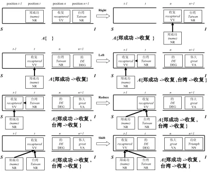
Example: 䚥៤ࡳᬊৄⱘӳࡳϮ (The great triumph that Cheng Cheng-Kung recaptured Taiwan.)
Fig. 1. The operations of the Nivre algorithm ᬊ position t-1 position t position n position n+1
2.1 Algorithm
We utilize a bottom-up deterministic algorithm proposed by (Nivre and Scholz, 2004) in our analyzer. In the algorithm, the states of analyzer are represented by a triple S,I,A .S and I are
stacks,Skeeps the words being in consideration, andI keeps the words to be processed. A is a list of dependency relations decide during the algo-rithm. Given an input word sequence W, the analyzer is initialized by the triple nil,W,
φ
.The analyzer estimates the dependency relation between two words (the top elements of stack S and stack I). The algorithm iterates until the list I becomes empty. Then, the analyzer outputs the word dependency relations A.
There are four possible operations for the con-figuration at hand:
Right: Suppose the current triple is A
I n S
t| , | , (t and n are the top elements, S and I are the remaining elements in the stacks), if there is a dependency relation that the word t depends on word n, add the new dependency relation
(
t→n)
into A, remove t from S. The configuration now becomes S,n|I,A{
(
t→n)
}
.Left: In the current triple is t|S,n|I,A , if there is a dependency relation that the word n depends on the word t, adds the new dependency relation
(
n→t)
into A, push n onto the stack S.The configuration now becomes
(
)
{
n t}
A I S t
n| | , , → .
Suppose the current triple is t|S,n|I,A , if there is no dependency relation between nand t, check the following conditions.
Reduce: If there are no more words n' (n'∈I) which may depend on t, and t has a parent on its left side, the analyzer removes t from the stack S. The configuration now becomes S,n|I,A . Shift:If there is no dependency between nand t, and the triple doesn’t satisfy the conditions for Reduce, then push n onto the stack S. The con-figuration now becomes n|t|S,I,A .
These operations are depicted in Fig. 1. Given an input sentence of length N (words), the ana-lyzer is guaranteed to terminate after at most 2N actions. The dependency structure given at the termination is well-formed if and only if the re-lations in A constitute a single connected tree.
This means that the algorithm produces a well-formed dependency graph.
2.2 Machine learning method
A classification task usually involves with train-ing and testtrain-ing data which consist of annotated data instances. Each instance in the training set contains one “target value” (class label) and several “attributes” (features). The goal of a classifier is to produce a model which predicts target value of data instances in the testing set which only give the attributes.
SVMs are binary classifiers based on the maximal margin strategy. Suppose we have a set of training data for a binary classification prob-lem: (Z1,y1)...(Zn,yn), where
n R
∈
i
Z is the fea-ture vector of the i-th sample in the training data and yi∈{+1,−1}is the class label of the sample. The goal is to find a decision function
) ) ( (
)
(
¦
∈
+ =
SV i i
i
b K
y a sign x f
\
i
,\
Z for an input
vec-tor
Z
. The vectors \K∈SV are called support vectors, which are representative examples. Support vectors and other constants are deter-mined by solving a quadratic programming problem. K(x,z)is a kernel function which maps vectors into a higher dimensional space. We usethe polynomial kernel: d
K(x,z)=(1+x⋅z) . The performance of SVMs is better than using other machine learning methods, such as memory based learning or maximum entropy method, in our analyzer. This is because that SVMs can adopt combining features automatically (using the polynomial kernel), whereas other method cannot. To extend binary classifiers to multi-class multi-classifiers, we use the pair-wise method, which utilizes nC2 binary classifiers between all pairs of the classes (Kreel, 1998). We use Libsvm (Lin et al., 2001) in our experiments.
2.3 Features (Local features)
It should be noted that we use a different ma-chine learner from the original method (Nivre, 2004). Nivre’s work used memory based learn-ing in their analyzer, we utilize SVMs in our analyzer. Therefore, the features of our analyzer are different from the original Nivre’s method.
triple. The nodes include the word, the POS-tag and the information of its children. The context features we use are 2 preceding nodes of node t (andt itself), 2 succeeding nodes of node n(and n itself), and their child nodes. The distance be-tween nodes n and t is also used as a feature. We call these features as local features.
3 Global features and two-step process
In the algorithm, the operation Reduce needs the condition that the node n should have no child in I. However, it is difficult to check this condition. In a long sentence, the modifier of the focused node n may be far away from n. More-over, some non-local dependency may cause this kind of error. In this section, we will describe this problem and a solution to it.
3.1 Global features
The analyzer selects features for deciding the optimum operation, and then gives these fea-tures to machine learner. The machine learner uses the same information to decide the opti-mum operation even when these operations es-sentially disagree. However, the different operation consists of different condition. In the deterministic bottom-up dependency analysis, we can generally consider the process as two tasks:
Task 1: Does the focused word depend on a neighbor node?
Task 2: Does the focused word may have a
child in the remaining token sequence?
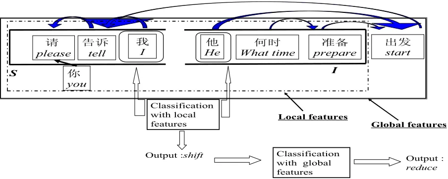
In the Task 1, the problem can be resolved by using the information of the neighbor nodes. This information is possibly the same as the fea-tures that we described in section 2.3. However, these features may not be able to resolve the problem in task 2. For resolving the problem in task 2, we need the information of long distance dependency. In Fig. 2, for example, the analyzer is considering the relation between focused words “ਞ䆝 (tell)” and “Ҫ (he)”. The features used in this original analysis are the information of words “䇋 (please)”, “ਞ䆝 (tell)”, “Ҫ(he)”, “ԩᯊ (what time)” and “ޚ (prepare)”. These features are “local features”. The correct answer in this situation is the operation “Shift”. It is because the word “ਞ䆝 (tell)” has a child “ߎথ
(start)” which is not yet analyzed and the fo-cused words don’t depend on each other. How-ever, the local features do not include the information of word “ߎথ (start)”. Therefore, the analyzer possibly estimates the answer as the operation “Reduce”. The results make a mistake in this situation because of the lack of long dis-tance information. To resolve this problem, we should refer some information of long distance dependency in machine learning. The informa-tion about long distance relainforma-tions is defined as “global features”. In this paper, we select the words which remain in stack I but don’t be con-sider in local features as global features.
Fig. 2. An example of the ambiguity of deciding the long distance dependency relation and using two-steps classification dependency relation
ޚ prepare 䇋
please
Դ you
ਞ䆝 tell
៥ I
ԩᯊ What time
ߎথ start Ҫ
He
S I
(Please tell me what time he will prepare to start.)
Classification with local features
Output :shift
Local features
Global features
Classification with global features
Output :
3.2 two-step process
To use the global features, we cannot use them immediately because the global features are not effective in all operations. For using global fea-tures efficiently, we propose a two-step process in our analyzer. The analysis processes are di-vided to two processes. First, the analyzer uses only the local features (as described in Section 2.3) to decide the optimum operation. If the re-sult is “Reduce” or “Shift”, it means that the focused words do not have any dependency rela-tion. The analyzer leaves the decision to another machine learner that makes use of global fea-tures. The analyzer will select global features for analyzing the Task 2. Then the analyzer outputs the final answer of this analysis process.
Fig. 2 describes an example of using two-step classification for analyzing dependency relation. In this example, the focused words are “៥ (I)” and “Ҫ (He)”. The word “៥ (I)” depends on the word “ਞ䆝 (tell)”. The local features are surrounded by dotted line and the global features are surrounded by solid line. The analyzer used local features to analyze the operation of this situation. The result is the operation “shift”. The analyzer then selected the global features to ana-lyze again and the output is the operation “ re-duce”. The final result of this situation is the operation “reduce”.
4 The root node finder
In Isozaki’s work (Isozaki et. al, 2004), they adopted a root finder in their system to find the root word of the input sentence. Their method used the information of the root word as a new feature for machine learning. Their experiments showed that information of root word was a beneficial feature. However, we think the infor-mation of root word can be used not only as the feature of machine learning, but also can be used to divide the sentence. Therefore, the complex-ity of the sentence can be alleviated by dividing the input sentence.
4.1 Root node and dividing sentence by using root finder
In the fundamental definition of dependency structure, there is one and only one head word in a dependency structure. An element cannot have
dependents lying on the other side of its own governor.
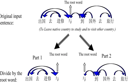
These peculiarities imply that the head word divides the phrase into two independent parts and each part does not cross the head word. As in Fig. 3, the original input sentence has a root word (the head word of phrase) “Ϣ(and)”. There are not any dependency relation which crosses the root word. Therefore we can divide this sentence into two sub-sentence “ߎ ( exo-dus) / এ (do) / 䖯ׂ (study) / Ϣ (and)” and ”Ϣ (and) / ࠄ (go) / (foreign country) / এ(do) / ᮙ㸠 (visit)”. Both these sub-sentences have their root word and the root word is ”Ϣ(and)”. We can conceive that to analyze the dependency structure of the full sentence is to analyze the dependency structure of two sub-sentences. Combining structures of two sub-sentences, we can get the full structure of original sentence. Our dependency analyzer is a bottom-up deter-ministic analyzer. Instinctively, the accuracy of analyzing short sentence is significantly better than analyzing long sentence. Thus the perform-ance of the dependency analyzer can be im-proved by this method.
4.2 Constructing a root finder
To use the root node, we should construct the root finder. Similarly to Isozaki’s work, we use machine learner (SVMs) to construct the root finder. We refer to the features which are used in Isozaki’s work and investigate other effective features. The performance of our root node finder is 90.71%. This is better than the root ac-curacy of our analyzer (86.22%, see Table 2).
Fig. 3. Dividing the phrase as two phrases by the root word
ߎ এ 䖯ׂ Ϣ ࠄ এ ᮙ㸠
(To Leave native country to study and to visit other country.)
The root word
ߎ এ 䖯ׂ Ϣ Ϣ ࠄ এ ᮙ㸠
The root word The root word
Original input sentence:
Divide by the root word:
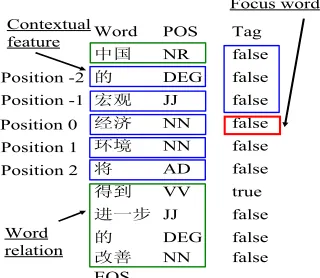
Therefore, using the root finder can give the de-pendency analyzer more top-down information. The tags and features of the root finding are shown in Fig. 4. We extract all root words in the training data and tagging every word to show that it is root word or not. For example, the root word in Fig. 4 is “ᕫࠄ (get)”. The root finder analyzes each word in the sentence and gives the tag “true” or “false” to indicate the root word. The features for machine learning of root finder include the contextual features (the information about the focused word, the two preceding words, and two succeeding words) and the word relation features (the words which are in the out-side of the window). Other effectual features include the Boolean features “root word is found” and “the focus word is the first/last word of sentence”. For example, the contextual fea-tures of the word “㒣⌢ (economic)“ include information of the focused (n) word “㒣⌢ ( eco-nomic)”, the “n-1”th word “ᅣ㾖 (wide)”, the “n-2”th word ”ⱘ (DE)”, the “n+1”th word” ⦃
๗ (environment)” and the “n+2”th word ”ᇚ (will)”. The word relation features include the preceding word set {Ё (China)}, the suc-ceeding word set {ᕫࠄ, 䖯ϔℹ,ⱘ,ᬍ} and
the Boolean features are:
“root_word_is_found=false”,
“first_word=false” ,”last_word=false”.
When we use the root finder to analyze the root word of the sentence, we do not know the structure of input sentence (either the phrase structure or the dependency structure). It may look odd that the root finder can analyzes the root word without any information of the struc-ture. However, this analysis is practicable. Natu-rally, the root word of a sentence is usually a verb (about 61% of sentences have a verb as the root word in our testing corpus). For example, in
the example 1 of Fig. 5 “៥ / এ / ᄺ᷵ (I go to school)”, we know the POS-tags are “noun, verb, noun” thus we can find that the root word is ”এ (go)”. However, many sentences include more then one verb or the root word is not verb (in NP or PP…etc.). We can not only choose the verbs as root word directly. To decide the root word of complex sentences, there are some special word/POS relations that can be used to estimate the root node of a sentence. Considering the root finder in Fig. 4, the root finder gives the root tag to each word of the sentence.
The processes of analyzing the root word can be thought as two tasks:
Task 1: Does the focus word depend on a neighbor word?
Task 2: Are there any special relation in the sen-tence?
In Fig. 4, the contextual features (two pre-ceding words and two succeeding words) can be used to process the Task 1, and the word rela-tion features can be used to process the Task 2. If the focused word possibly depends on neighbor words, it is impossible that the focused word is the root word. Therefore these words will be tagged as “false”.
Alternately, considering the example 2 in Fig. 5, the sentence has a verb “ᬊ (recapture)”, but the special word “ⱘ (DE)” is in the right side of the verb “ᬊ (recapture)”. Therefore, the verb “ᬊ (recapture)” is possibly in theⱘ
(DE)-phrase and the verb cannot be the root word. The special word “ⱘ (DE)” resembles a preposition and it is always the last word of DE-phrase. Therefore, although we do not know the structure of sentence, we can identify which words can be the root word by the relation and position of the features. If the features of the focused word include the special word relations
Word POS Tag
Ё NR false
ⱘ DEG false
ᅣ㾖 JJ false
㒣⌢ NN false
⦃๗ NN false
ᇚ AD false
ᕫࠄ VV true
䖯ϔℹ JJ false
ⱘ DEG false
ᬍ NN false
EOS Position 0 Position -1 Position -2
Position 1
Position 2
Focus word Contextual
feature
Word
relation Fig. 5. The examples of analyzing the root word
of sentences
Root
䚥៤ࡳ ᬊ ৄ ⱘ ӳ ࡳϮ
NR VV NR DEG VA NN
(The great triumph that Cheng Cheng-Kung recaptured Taiwan. )
៥ ᄺ᷵
DT VV NN
(I go school.) Root
Example 1:
(for example, the focused word is in the preposi-tional phrase), it isn’t the root word. The fea-tures “word relations” in Fig. 5 can consider this situation.
5 Experiments
5.1 Corpus and estimation
We use Penn Chinese Treebank 5.0 (Xue et al., 2002) in our experiments. This Treebank is rep-resented by phrase structure and doesn’t include the head information of each phrase. The first step of using Penn Chinese Treebank is to derive the head rules for deciding the head word of each phrase. Some examples of head rules are shown in Table 1. We convert the Treebank by using these head rules. The training corpus in-cludes about 377,408 words for learning and 63,886 words for testing. It should be noted that the punctuation mark “DŽ” marks the end of a sentence in the Treebank. However, the punc-tuation mark “‚” also can be the end of a sen-tence. It is hard to determine the dependency rule of the clauses on the both side of comma. Therefore, to decide the dependency relation which crosses a punctuation mark “‚” is difficult. We do not deal with the ambiguity of commas and divide the sentence by the punctuation mark “‚”.
Phrase The order of deciding the head of phrase (from left)
ADJP CC PZ ADJP JJ
ADVP CC PZ AD
CLP PZ CLP M LC
DP DP CLP QP DT
DVP DEV DEC DEG
VCP VC VV
Table 1. Some examples of head rules
The performance of our dependency structure analyzer is evaluated by the following three measures:
Dependency Accuracy:
relations dependency
of number
relations dependency
analyzed correctly
of number
=
Root Accuracy:
clauses of number
nodes root analyzed correctly
of number
=
Sentence Accuracy:
clauses of number
clause analyzed correctly
fully of number
=
5.2 Results and discussion
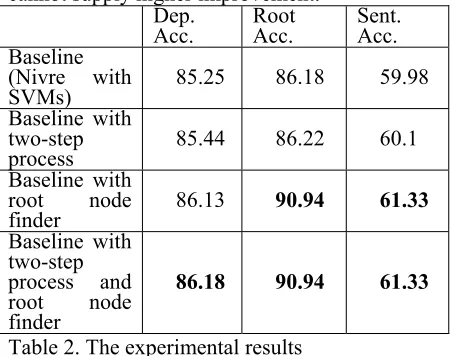
Our experimental results are shown in Table. 2. First row in the table is the result of our basic analyzer (Nivre algorithm with SVMs), second and third row show the effects of the proposed extensions. The last row is the result of combin-ing the two extensions. We had used McNemar test to confirm the significance of the methods. The McNemar test proves that using the pro-posed methods improve the analyzers signifi-cantly. Comparing the results of our basic analyzer to related works, our analyzer (dep. Accuracy: 87.64) is better than (Ma et al., 2004, dep. Accuracy: 80.38) and (Zhou, 2000, dep. Accuracy of newspaper: 67.7). However, these researches used different corpus. We cannot compare the performances directly.
According to the second row of Table. 2, di-viding the process of classification as two steps can improve the performance of dependency analyzer. However, the improvement of using this method is limited. This is because that long distance relations are not many in the corpus. The absence of global information does not oc-cur in the sentences without long distance rela-tions. Another reason is the distribution of operations. The instances of operations in our experimental corpus are not balanced. The op-eration “reduce” is the least (7.8%) and it is far less than other operations. Therefore the in-stances for creating the model of operation “ re-duce” are not satisfactory. These facts result in that our experiment of using two step classifica-tion cannot improve the analyzer remarkably.
About the experiment of utilizing root finder in our analyzer, we tried to adopt the root infor-mation to the analyzer (using the inforinfor-mation as features for machine learning). However, the performance is worse than the baseline (the fun-damental analyzer “Nivre+SVMs”). Therefore, we use our method to improve the analyzer by using root information (dividing the sentence according to root node).
The last row of Table. 2 shows the results of combining the two proposed methods (using global features and root node finder) to improve our analyzer. Combining two methods can in-crease the dependency accuracy better than us-ing either one of the methods. It means that some analysis errors of fundamental analyzer can be resolved by using both improvement methods. Therefore using combined method cannot supply higher improvement.
Dep. Acc.
Root Acc.
Sent. Acc. Baseline
(Nivre with
SVMs) 85.25 86.18 59.98
Baseline with two-step
process 85.44 86.22 60.1
Baseline with root node
finder 86.13 90.94 61.33
Baseline with two-step process and root node finder
86.18 90.94 61.33
Table 2. The experimental results
6 Conclusion and future work
In this paper, we present two methods to im-prove a deterministic dependency structure ana-lyzer for Chinese. This basic anaana-lyzer implements a bottom-up deterministic algorithm with SVMs. We convert a phrase structure anno-tated corpus (Penn Chinese Treebank) to de-pendency tagged corpus by using head rules. According to the properties of Chinese language and dependency structure, we try to add a root finder in our dependency analyzer to improve the analyzer. Moreover, considering the machine learning process of our analyzer, we divide the process into two processes to improve the per-formance of analyzer. The improving methods (using root finder and dividing machine learning process) showed to improve the analyzer.
Future work includes three points. First, we should improve the performance of the root finder. Second, we should construct a useful prepositional phrase chunker, because the prepositional phrase is a major error source of our basic analyzer. The original analyzer tends to let the preposition governing a partial subtree of the full phrase. According to the properties of Chinese language, the prepositional phrases in Chinese are head-initial. Intuitively, if we can extract the prepositional phrases from sentence, the complexity of the sentence will decrease.
Thus an important task is how to chunk the prepositional phrase in the sentence.
Finally, we should deal with the ambiguity of the meaning of punctuation mark “,”. The defi-nition of “sentence” is ambiguous in Chinese. In Chinese articles, the normal ending mark of a sentence is the punctuation mark “DŽ”. However, the mark “‚” is often used at the end of a sen-tence. To distinguish the meaning of the punc-tuation mark “‚” is difficult. Therefore, we should adopt semantic analysis in our analyzer.
References
1. Eugene Charniak, 2001. Immediate-Head Parsing for Language Models. pages 124-131, NAACL-2001.
2. Yuen Ren Chao, 1968. A Grammar of Spoken Chinese. Berkeley, CA: University of California Press.
3. Michael Collins, Brian Roark, 2004, Incremental parsing with the Perceptron algorithm. Pages 112-119, ACL-2004.
4. J. Huang, 1982. Logical relations in Chinese and the theory of grammar Doctoral dissertation, Mas-sachusetts Institute of Technology, Cambridge. 5. Ulrich. H.-G. Kreȕel, 1998. Pairwise classification
and support vector machines. In Advances in Kernel Methods, pages 255–268. The MIT Press. 6. Chih Jen Lin, 2001. A practical guide to support
vector classification, http://www.csie.ntu.edu.tw/ ~cjlin/libsvm/.
7. Lai, Bong Yeung Tom, Huang, Changning, 1994. Dependency Grammar and the Parsing of Chinese Sentences. PACLIC 1994
8. Hideki Isozaki, Hideto Kazawa, Tsutomu Hirao, 2004. A Deterministic Word Dependency Ana-lyzer Enhanced With Preference Learning, pages 275-281, COLING-2004
9. Charles Li, and Thompson Sandra A., 1981. Man-darin Chinese. University of California Press. 10. Lin-Shan Lee, Long-Ji Lin, Keh-Jiann Chen, and
James Huang, 1991. An Efficient Natural Lan-guage Processing System Specially Designed for the Chinese Language. ComputationaI Linguistics, Volume 17, Number 4.
11. Ma Jinshan, Zhang yu, Liu ting, and Li sheng, 2004. A Statistical Dependency Parser of Chinese-under Small Training Data. IJCNLP 2004 Work-shop: Beyond shallow analyses, Formalisms and statistical modeling for deep analyses.
12. Joakim Nivre and Mario Scholz, 2004. Determi-nistic Dependency Parsing of English Text. Pages 64-70, COLING-2004.
13. Adwait Ratnaparkhi, 1999. Learning to parse natural language with maximum entropy models. Machine Learning, 34(1-3) pages151–175.
14. Vladimir N. Vapnik, 1998. Statistical Learning Theory. A Wiley-Interscience Publication. 15. Nianwen Xue, Fu-Dong Chiou, Martha Stone
Palmer, 2002. Building a Large-Scale Annotated Chinese Corpus. COLING 2002